Article

Hyperparameter Bayesian Optimization of Gaussian Process Regression Applied in Speed-Sensorless Predictive Torque Control of an Autonomous Wind Energy Conversion System

1
Laboratoire de Maitrise des Energies Renouvelables (LMER), Faculté de Technologie, Université de Bejaia, Bejaia 06000, Algeria
2
Department of Electric, Electronics and System Engineering, Faculty of Engineering and Built Environment, Universiti Kebangsaan Malaysia, Bangi 43600, Malaysia
3
Fukushima Renewable Energy Institute, AIST (FREA), National Institute of Advanced Industrial Science and Technology (AIST), Koriyama 963-0298, Japan
*
Authors to whom correspondence should be addressed.
Energies 2023, 16(12), 4738; https://doi.org/10.3390/en16124738
Submission received: 7 May 2023 / Revised: 10 June 2023 / Accepted: 14 June 2023 / Published: 15 June 2023
(This article belongs to the Special Issue Wind Energy Generation and Wind Turbine Models)

Abstract

:
This paper introduces a novel approach to speed-sensorless predictive torque control (PTC) in an autonomous wind energy conversion system, specifically utilizing an asymmetric double star induction generator (ADSIG). To achieve accurate estimation of non-linear quantities, the Gaussian Process Regression algorithm (GPR) is employed as a powerful machine learning tool for designing speed and flux estimators. To enhance the capabilities of the GPR, two improvements were implemented, (a) hyperparametric optimization through the Bayesian optimization (BO) algorithm and (b) curation of the input vector using the gray box concept, leveraging our existing knowledge of the ADSIG. Simulation results have demonstrated that the proposed GPR-PTC would remain robust and unaffected by the absence of a speed sensor, maintaining performance even under varying magnetizing inductance. This enables a reliable and cost-effective control solution.

1. Introduction

Renewable energy sources offer a promising solution to address the challenges of increasing energy demand and global climate change [1,2]. The generation of electricity from wind energy is widely recognized as a rapidly growing industry on a global scale [3,4]. Wind energy is highly efficient and abundant, making it a valuable source of electricity. In isolated areas, autonomous wind power systems require storage solutions to address intermittency. Batteries, connected to a system’s DC bus via a DC/DC converter, are commonly used for this purpose, as in [5,6,7]. The introduction of multiple stator winding machines has opened up possibilities for considering alternative structures. One such structure involves dedicating one stator star to storage, so that a battery is connected through an inverter, and dedicating the second stator star to power, supplying the load. This particular structure was developed by the authors of [8]. The proposed structure in Figure 1 offers the advantage of achieving galvanic isolation between the two stator stars and allows for the independent control of each star. This feature makes this structure well-suited for this study. A simulation was performed using MATLAB/Simulink/SimPowerSystem with the ode45 (Dormand–Prince) solver. This simulation employed a variable step size, with a maximum step size of 1 × 10⁻³ s. The inverter was modeled using the IGBT element available in the SimPowerSystems toolbox, while the motor was represented using an abc mathematical equation. In the presence of magnetic circuit saturation, the double star induction generator (DSIG) would require a non-linear control strategy that could effectively adapt to this variation. In this paper, the chosen control approach is predictive torque control (PTC). PTC is particularly suitable for this application, as it is capable of handling magnetic saturation and offers several advantages. Notably, PTC is a relatively new control technique known for its simplicity and does not require the use of pulse width modulation. Furthermore, PTC is easily adaptable to incorporate various system constraints, making it a favorable choice for controlling the DSIG [9,10]. The principle of this control is based on the prediction of future torque and flux values, which allows it to be more flexible and have a faster dynamic response [11].
The implementation of PTC traditionally involves the installation of flux and speed sensors, leading to higher installation costs and reduced reliability. To address this limitation, various approaches have been proposed in the literature to replace mechanical sensors with speed estimators. These estimators offer the advantages of cost reduction and increased reliability. One such approach is the Model Reference Adaptive System (MRAS), which leverages the mathematical models of a machine to achieve accurate speed estimation [12,13,14,15]. Others include the Sliding Mode Observer (SMO) [16,17,18] and the Kalman Filter (KF) [19,20,21]. Observer-based approaches that employ simplified linear models of machines are often susceptible to parametric variations and external disturbances in real-world machines. While efforts have been made to enhance their robustness through the use of more accurate models or hybrid approaches, these improvements come at the cost of increased complexity and computational expenses [22].
The concept of the free model approach, utilizing machine learning (ML) algorithms, enables construction of non-linear estimators without the need for explicit knowledge of a system’s mathematical model. This approach treats the system as a black box and relies solely on the inputs and outputs of the system [23,24]. While the gray box approach has shown effectiveness with simple systems, it tends to yield poor results when applied to highly non-linear systems.
In previous studies, researchers have attempted to enhance the free model approach by incorporating system knowledge and making modifications to estimator inputs to increase their significance. This approach, known as the gray box approach, enables the development of highly accurate estimators [25,26]. The concept of utilizing ML algorithms for designing flux and speed estimators is adopted in this paper.
The choice of hyperparameters poses a significant challenge in ML training. While manually selecting hyperparameters can yield acceptable results, it often requires substantial human effort and limits the performance of the model. Since the gradient of the objective function cannot be computed analytically, researchers have opted to replace it with optimization algorithms. While grid search and random search are common hyperparameter optimization strategies, they can be computationally expensive, as they require a large number of function evaluations. In contrast, hyperparameter Bayesian optimization (HBO) offers a more promising approach [27,28,29,30]. It has emerged as a powerful solution to obtain the best possible configuration using a small number of function evaluations. Additionally, it has a wide range of applications, such as drug design [31], interactive user interfaces [32], robotics [33,34], inversion problems [35,36], environmental monitoring [37], information extraction [38], combinatorial optimization [39], automatic machine learning [40,41], sensor networks [42], adaptive Monte Carlo (MC) [43], experimental design [44], and reinforcement learning [45]. The compelling advantages of the Gaussian Process Regression algorithm (GPR) described above served as the motivation for adopting this algorithm in this paper.
Various supervised machine learning algorithms can be employed as surrogate models for Bayesian optimization (BO), including linear regression, support vector machines, the Gaussian Process, ensemble learning, ANNs, and decision trees. In this paper, we specifically utilized the GPR algorithm for speed and flux estimations. The application process and hyperparameter optimization remain the same for any multivariate function, with the distinction being in the choice of input based on the gray box principle. The machine utilized has a nominal power of 8 kW, with 2 kW allocated for storage winding and 6 kW allocated for power winding. Table 1 presents the specifications and corresponding values of the machine.
The primary objective of this study was to develop a robust flux and speed estimation technique using GPR, thereby enhancing the PTC implemented in an autonomous wind energy production system. To fully leverage the capabilities of GPR, we incorporated two key enhancements: (a) HBO and (b) input vector curation based on the concept of the gray box. With these improvements, we aimed to achieve higher accuracy in the estimation process and enable the system to adapt to the parametric variations of the asymmetric double star induction generator (ADSIG) without requiring detailed knowledge of its underlying model.
This article presents the following key contributions and objectives in detail:
  • Enhancement of controller reliability;
  • Adaptation to variations in magnetizing inductance;
  • Improved accuracy of the estimator through the implementation of HBO and the gray box approach;
  • Reduction of overall system costs;
  • Mitigation of harmonics through the introduction of galvanic isolation between the two stars.
These contributions and objectives are thoroughly explored and discussed in the subsequent sections of the article. This document is structured as follows: Section 2: the ADSIG mathematical model with saturation; Section 3: GPR supervised learning algorithms and optimization; Section 4: sensorless PTC theory for the ADSIG; Section 5: results analysis of the GPR training phase; Last section: simulation results interpretation and performance analysis. These sections cover the ADSIG model, GPR algorithms, sensorless PTC theory, analysis of training results, and interpretation of simulation outcomes.

2. ADSIG Modeling

The machine used is composed of two non-identical stator windings. The first is called the storage winding and constitutes 25%, and the other is called the power winding and takes 75% of the stator winding. The rotor is a squirrel cage, but for simplification reasons, it is considered a short-circuited three-phase winding. The stator and rotor voltages are expressed as the following complex equations [46]:
v ¯ s 1 = r s 1 ı ¯ s 1 + d d t φ ¯ s 1 v ¯ s 2 = r s 2 ı ¯ s 2 + d d t φ ¯ s 2 v ¯ r = r r ı ¯ r + d d t φ ¯ r j ω r φ ¯ r = 0
where v s x x = 1 , 2 ;   v r : the stator, rotor voltage; r s x x = 1 , 2 ;   r r : the stator, rotor resistance;   ω r : the rotor electrical angular speed; φ s x x = 1 , 2 ;   φ r : the stator, rotor flux linkages; ı s x x = 1 , 2 ;   and   ı r : the stator, rotor current. All other symbols stand for their usual meanings. The expressions of the stator and rotor flux linkages are as follows [47]:
φ ¯ s 1 = L l s 1 ı ¯ s 1 + L m ı ¯ s 1 + ı ¯ s 2 + ı ¯ r φ ¯ s 1 = L l s 2 ı ¯ s 2 + L m ı ¯ s 1 + ı ¯ s 2 + ı ¯ r φ ¯ r = L l r ı ¯ r + L m ı ¯ s 1 + ı ¯ s 2 + ı ¯ r
where L l x ( x = s 1 , s 2 , r ): stator (respectively, rotor) leakage inductance; L m : magnetizing inductance; and both armatures (stator and rotor) are smooth poles.
Magnetic circuit saturation is a non-linear phenomenon that can be modeled by a variable magnetizing inductance expressed by a polynomial equation determined after an experimental test. The magnetization inductance, L m , as a function of the magnetizing current, ι m , is approximated by [48,49]:
L m = 0.1406 + 0.0014   ı m 0.0012   ı m 2 + 0.00005   ı m 3
The expression of the magnetizing current is given by [48]:
ı m = R e ( ı ¯ s + ı ¯ r ) 2 + I m ( ı ¯ s + ı ¯ r ) 2
With
ı ¯ s = ı ¯ s 1 + ı ¯ s 2
The electromagnetic torque is given by:
T e m 1 = P   I m φ ¯ s 1   ı ¯ s 1   T e m 2 = P   I m φ ¯ s 2   ı ¯ s 2  
where φ ¯ s 1 and φ ¯ s 2 are the conjugates.
T e m = T e m 1 + T e m 2
where   T e m x x = 1 , 2 : the first and second stator winding torque; T e m : the total electromagnetic torque; and P : the number of pole pairs.
The machine mechanical equation is defined by:
T e m T g = J d Ω dt + f Ω
where   T g   : generator torque; Ω : the machine’s mechanical speed; J : inertia; and   f : viscous friction.

3. Gaussian Process Regression Theory

GPR is a robust and flexible machine learning method that utilizes a non-parametric probabilistic kernel model. In recent years, it has gained significant popularity in the literature [50]. Unlike many other machine learning models that provide a single prediction given the input, GPR offers a full distribution, which includes information about prediction uncertainty. This feature of GPR can be highly advantageous when making decisions based on predictions, as it allows for a more comprehensive understanding of the uncertainty associated with predictions.
The Gaussian Process is an extension of Gaussian probability distribution. While Gaussian distribution calculates the probability of an input vector based on its mean and variance, the Gaussian Process generalizes this concept, allowing for more flexible modeling and prediction. This is represented mathematically by Equation (9) [51]. The g function is distributed as a Gaussian Process, g p , which is specified by a mean function (the prediction),   μ x (Equation (10)), and a covariance function, k x , x (Equation (11)):
g x ~ g p μ x , k x , x  
μ x = E g x  
k x , x = E g x μ x g x μ x  
where E : the expectation.
To simplify the process and avoid complicated calculations, the mean function was initialized to zero, as depicted in Figure 2.
The kernel function that calculates covariance, k x , x , is determined directly with the Bayesian optimization algorithm. The kernel function fixed by the BO for this application is the rational quadratic equation for the speed estimator (Equation (12)) and Matern 5/2 for the flux estimator (Equation (13)) [52].
K R Q x i , x j = σ f 2 1 + r 2 2 α σ l 2 α
K M a t x i , x j = σ f 2 1 + 5 r σ l + 5 r 2 3 σ l 2 e x p 5 r σ l
where r = x i x j T x i x j : the Euclidean distance between x i and x j ; σ f : the signal standard deviation; σ l : the characteristic length scale; and α : a positive-valued scale-mixture parameter.
Hyperparameter Bayesian optimization and the gray box approach were employed to improve the GPR’s performance, as detailed in the following sections.

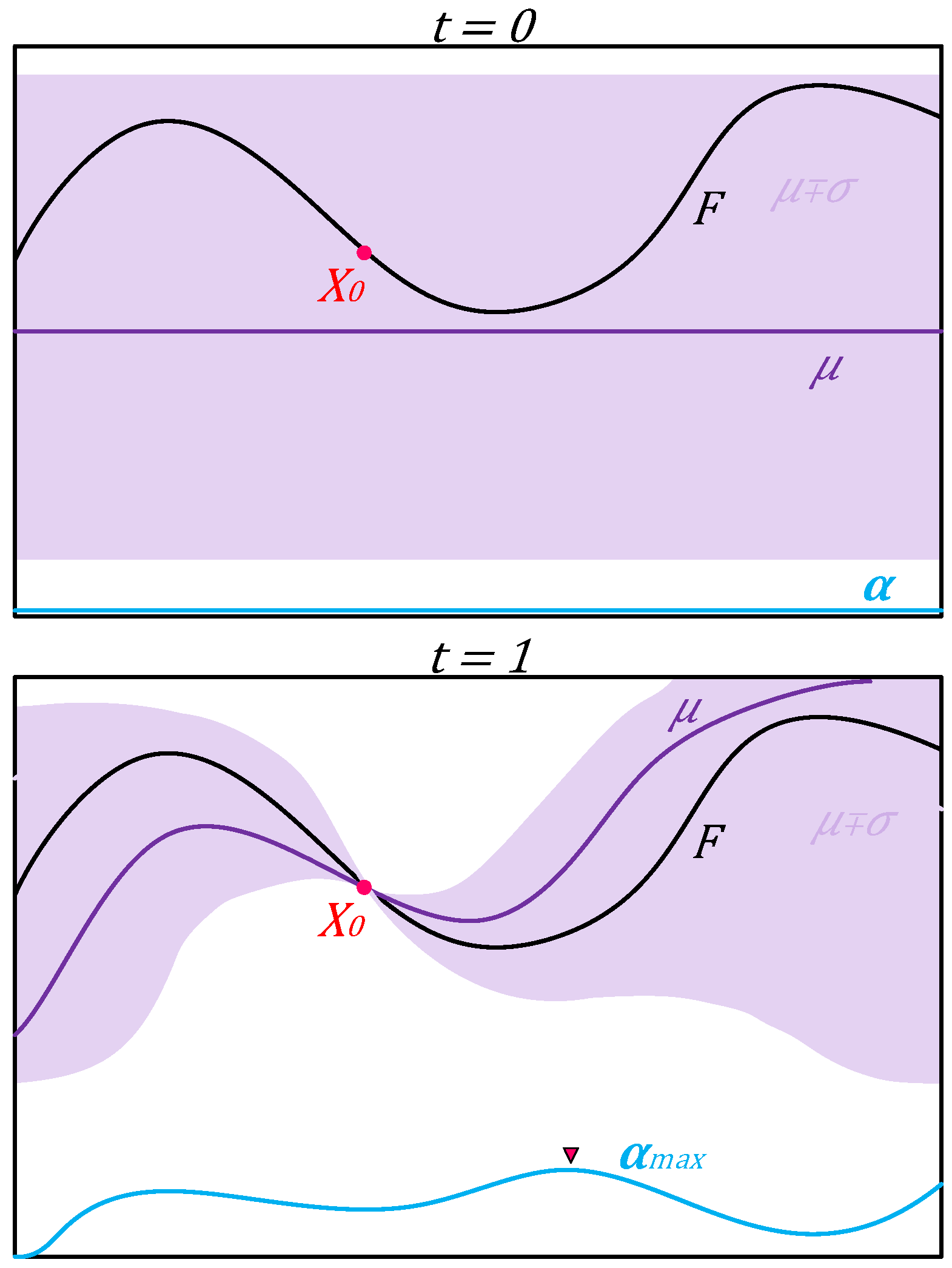
3.1. Hyperparameter Bayesian Optimization

In hyperparameter optimization utilizing the BO algorithm, in the beginning, it is necessary to define an initial set of configurations, X 0 (input value determined using the gray box principle described in the next section), and their associated function (in our case, the machine flux and speed value): D 0 = X 0 , y 0 . Then, in a loop, we updated the GP model using the Bayes rule; see [53,54]. Subsequently, a new hyperparameter configuration was chosen through the optimization of an auxiliary function known as the acquisition function. In this study, we specifically employed the expected improvement per second plus (EI+) as the selected acquisition function, as defined in Equation (14):
α t x = g X b e s t μ X   C g X b e s t ; μ X + σ f X   N g X b e s t ; μ X ; σ f X μ X
where C : the normal cumulative distribution function of the standard distribution; N : the normal distribution function; and X b e s t : the best point.
This configuration was used to evaluate the target score function, g , to obtain a new numerical score: the combination x t , y t . The newly generated data were then incorporated into the current training set for the subsequent iteration. The databases used for training the GPR were acquired from simulations of wind speeds ranging from 3 m/s to 12 m/s. After all the iterations were completed, the hyperparameter configuration that corresponded to the lowest numerical score was chosen. The entire process is outlined in Algorithm 1, as depicted in the pseudocode.
Algorithm 1. Pseudocode of Bayesian optimization with the GP surrogate model.
1:  Input data D = X , Y
2:  Initial small set of data randomly chosen D 0 = X 0 , Y 0 from D
3:  Compute a probabilistic Surrogate Function (Gaussian Process) g in such a way
to find Y 0 = g X 0
4:  for iterations t = 1 , 2 , do
5:  Select a new data set D t = X t , Y t from D by optimizing the Acquisition
Function α (expected improvement per second plus. Equation (14)):
                  X t = arg   max x   α X ; D t
4:  Augment data set D t = D t 1 X t , Y t
5:  Evaluate the Surrogate Function g for D t to find Y t = g X t
7:  end for
Figure 2 depicts the first four iterations of this algorithm. With each iteration, the mean function progressively approaches the objective function, accompanied by a reduction in uncertainty.

3.2. Gray Box Principle

By employing the gray box principle, which consisted of exploiting our prior knowledge of the process to control it and make some transformations, we obtained more significant estimator inputs. The transformations used in our case are given in Equations (15)–(20) [25]. These new inputs were obtained from nonlinear transformations of the voltages and currents of the two stator windings [12,24,25]:
u 1 x = v ¯ s 1  
u 2 x = ı ¯ s 1
u 3 x = R e v ¯ s 1   ı ¯ s 1
u 4 x = I m v ¯ s 1   ı ¯ s 1
u 5 x = R e v ¯ s 1 ı ¯ s 1
u 6 x = I m v ¯ s 1 ı ¯ s 1
where x = 1   for the storage star and 2 for the power star; u 1 x : the voltage peak value; u 2 x : the current peak value; u 3 x : active power; u 4 x : reactive power; u 5 x : the winding resistance value; and u 6 x : winding reactance.

4. Model Predictive Torque Control

In this section, we introduce the core concept and control structure of the finite-set PTC applied for the ADSIG. This control presents one of the most common model predictive control theories, thanks to its fast dynamics and good torque response [9]. The implementation of sensorless PTC essentially involves three steps:
-
First are the estimation of the stator and rotor flux values and the machine’s rotation speed using the GPR algorithm, as are detailed in Section 3.
-
The second step concerns prediction of the electromagnetic torque and the stator flux value through the stator current prediction. In this step, the prediction is made using forward Euler discretization of the ADSIG model presented in Section 2 (Equations (1), (2) and (7)), as shown in Equations (21)–(23):
φ ¯ s 1 p K + 1 = φ ¯ s 1 K + T s v ¯ s 1 k r s 1   i ¯ s 1 k φ ¯ s 2 p K + 1 = φ ¯ s 2 K + T s v ¯ s 2 k r s 2   i ¯ s 2 k
ι ¯ s 1 p K + 1 = T s R σ 1 τ σ 1 + T s k r 1 τ r + j ω r k φ ¯ r k + v ¯ s 1 k + 1 T s / τ σ 1 ι ¯ s 1 k ι ¯ s 2 p K + 1 = T s R σ 2 τ σ 2 + T s k r 1 τ r + j ω r k φ ¯ r k + v ¯ s 2 k + 1 T s / τ σ 2 ι ¯ s 2 k
where: R σ i = R s i + R r k r 2   ;   τ σ i = σ ( L l s i + L m ) R σ i ;   k r = L m L r   ;   σ i = 1 L m 2 ( L l s i + L m ) L r .
T e m 1 p K + 1 = P   I m φ ¯ s 1 K + 1   ι ¯ s 1 p   K + 1 T e m 2 p K + 1 = P   I m φ ¯ s 2 K + 1   ι ¯ s 2 p   K + 1
-
The last step is the choice and design of the cost function. This depicts a multi-objective online torque and flux optimization. Several cost functions have been developed in the literature, but for this work, we chose the simplest one, represented in Equation (24), where g 1 is the storage winding cost function and g 2 is the cost function of the power winding:
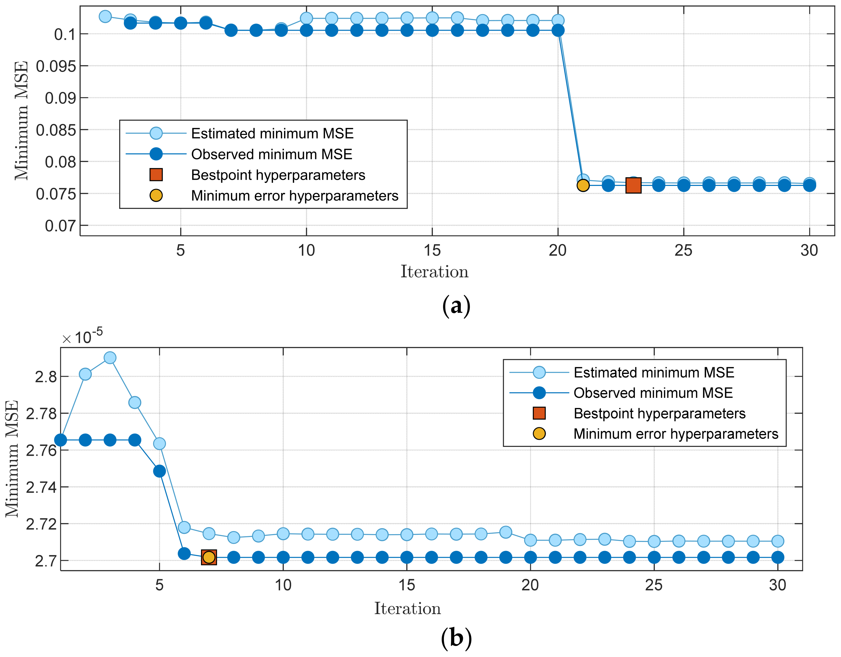
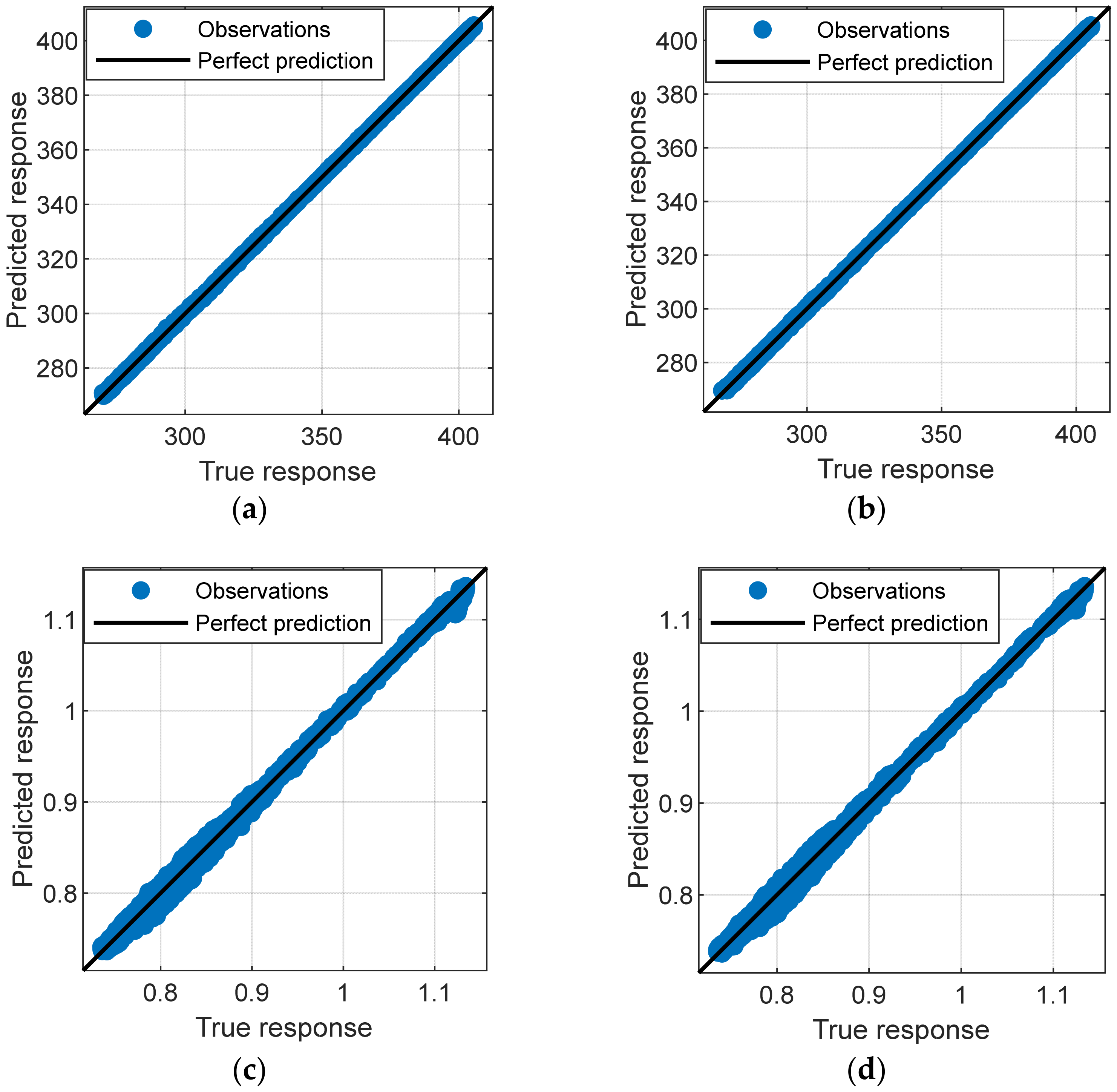
g 1 = T e m 1 T e m 1 p + λ φ s 1 φ s 1 p g 2 = T e m 2 T e m 2 p + λ φ s 2 φ s 2 p
To simplify the previous steps, a synoptic diagram is shown in Figure 3. The torque reference values, T e m 1 and T e m 2 , in the PTC were provided by the external loops (the green part): the speed regulation loop, to assure the MPPT, and the DC bus voltage regulation loop. Furthermore, the purple part includes the modifications introduced to the estimator inputs to make them more meaningful using the gray box principle.

5. Training Results

To estimate the values of the stator flux, the rotor flux, and the machine rotation speed, the GPR supervised learning method was applied. Three different databases were used in the training phase. The first database included 7876 examples used for training. The second database contained 1688 examples for validation, with the validation method chosen to examine the accuracy of the trained model and the holdout validation to protect it against overfitting, and the last database included 1688 examples used to evaluate model performance. The simulation was performed with MATLAB/Simulink software, using the solver ode45 (Dormand–Prince) and a maximum step size of 1 × 10⁻³ s.
The signal standard deviation was fixed at 0.1088 (standard value). The other hyperparameter of the GPR estimator was randomly initialized and optimized with the Bayesian hyperparameter optimization algorithm. The number of iterations was fixed to 30, and the acquisition function used was the expected improvement per second plus. To evaluate the performance of the GPR estimator, other supervised machine learning algorithms were trained in the same conditions cited above (Artificial Neural Network (ANN); support vector machine (SVM); ensemble learning (EL); and decision tree (DT)) [55,56,57,58,59].
Since we were confronted with a regression problem, to evaluate the accuracy of the estimator, it was not appropriate to calculate the number of prediction errors as in classification problems but to calculate the closest solution to the true values. There are several formulas for calculating this, but each method can fail in particular cases. to avoid this mistake, several indicators were examined at the same time, the Root Mean Square Error ( R M S E ); the coefficient of determination ( R 2 ); the Mean Square Error ( M S E ); and the Mean Absolute Error ( M A E ), in Equations (25)–(28), respectively:
R M S E = i = 1 n y ^ i y i 2 n  
R 2 = 1 i = 1 n y ^ i y i 2 i = 1 n y ˇ i y i 2
M S E = 1 n i = 1 n y ^ i y i 2
M A E = 1 n i = 1 n y ^ i y i
where n is the size of the database used for training, y i is the real (observed) response, and y ^ i is the predicted value.
The training results of the speed and flux estimators are presented in Table 2 and Table 3, respectively. These results demonstrate that the GPR method surpassed all other methods in terms of accuracy, with an estimation error of 0.07514 (2.5423 × 10⁻⁵) for speed and flux. This error is 24 (7) times lower than that of the closest algorithm, which is the ANN method, with an error of 1.7745 (1.66091 × 10⁻⁴).
Although the ANN algorithm achieved the fastest speed prediction, with 160,000 observations per second, and the SVM performed best for flux prediction, with 110,000 observations per second, the GPR prediction outperformed both methods significantly. The GPR method achieved a prediction rate of 3300 observations per second for speed and 5700 for flux, which is well above the maximum rectifier switch frequency. Therefore, the GPR method is the most suitable choice for this application. Bayesian optimization of hyperparameters enhances the performance of GPR compared to other algorithms. Specifically, compared to an alternative hyperparameter optimization algorithm, the GPR outperformed the ANN when Bayesian optimization was utilized.
Based on the compelling results obtained, the subsequent sections of this paper will concentrate on the implementation of the GPR estimator that was trained in the PTC wind power system.
Figure 4 illustrates the relationship between the Mean Square Error (MSE) and the iterations for the GPR estimates of both speed (a) and flux (b). The speed estimator reached the optimal hyperparameter point at iteration number 23, while the flux estimator achieved it after seven iterations. Table 4 provides the specific details of the best hyperparameters obtained for the GPR algorithm at these points.
To assess the performances of the flux and speed, a plot depicting the predicted versus actual values is presented in Figure 5. This plot shows the predicted responses plotted against the true responses. In an ideal regression model, where the predicted responses match the true responses, all data points would align perfectly on a diagonal line. The vertical distance from this diagonal line indicates the prediction error.
A reliable model exhibits minimal errors, meaning that the predictions would cluster closely around the diagonal line. It is worth noting that the estimated values align well with the line of perfect predictions represented by the diagonal line. This indicates that the model is not overfitted (based on the validation result) and demonstrates good generalization (based on the test result).

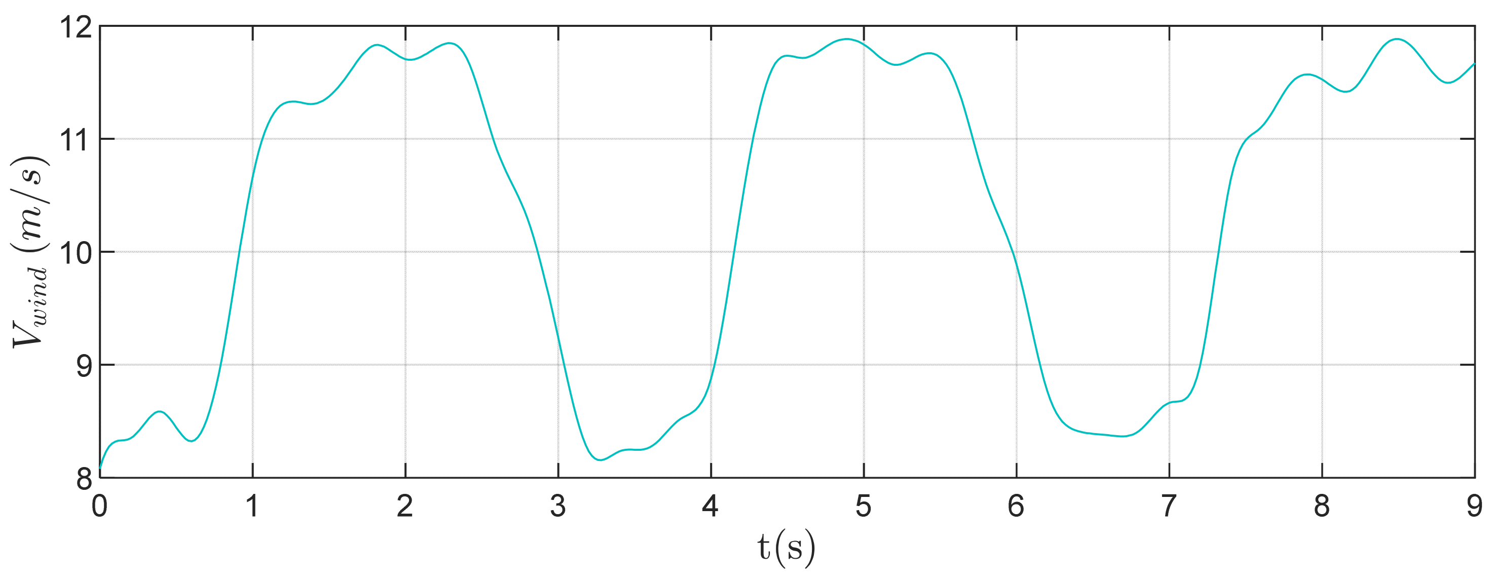
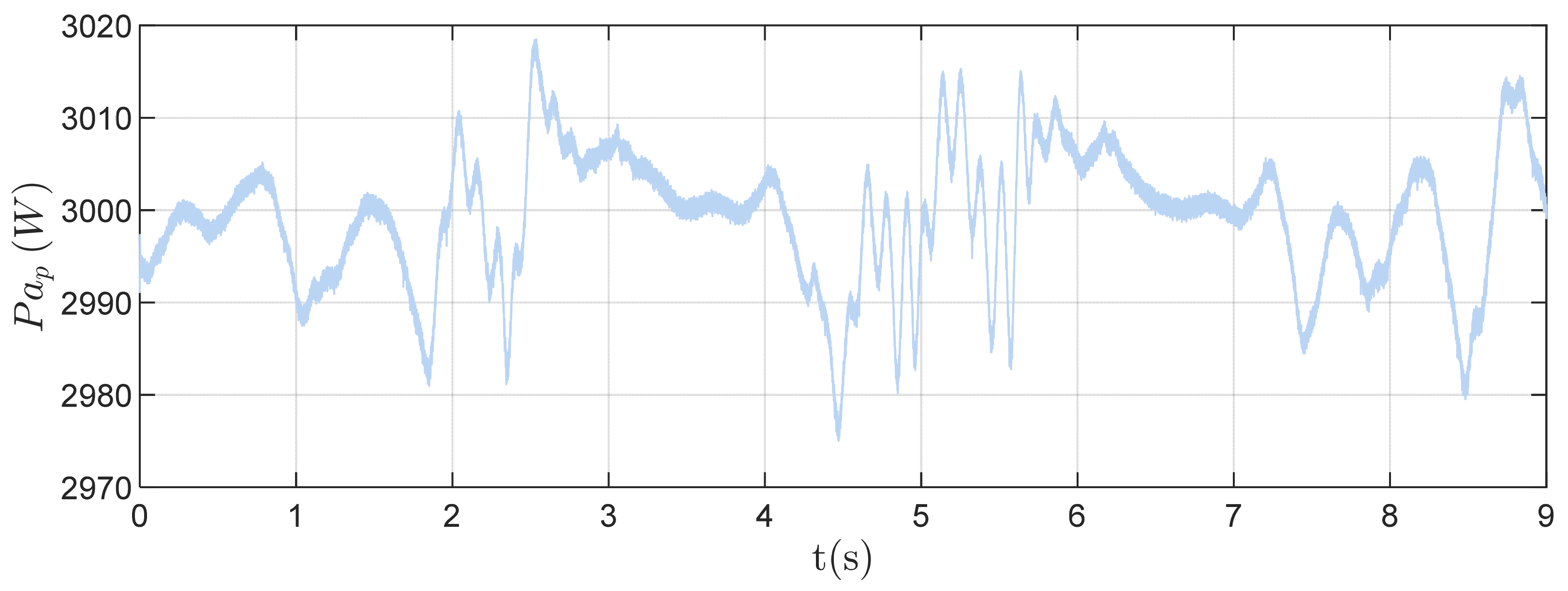
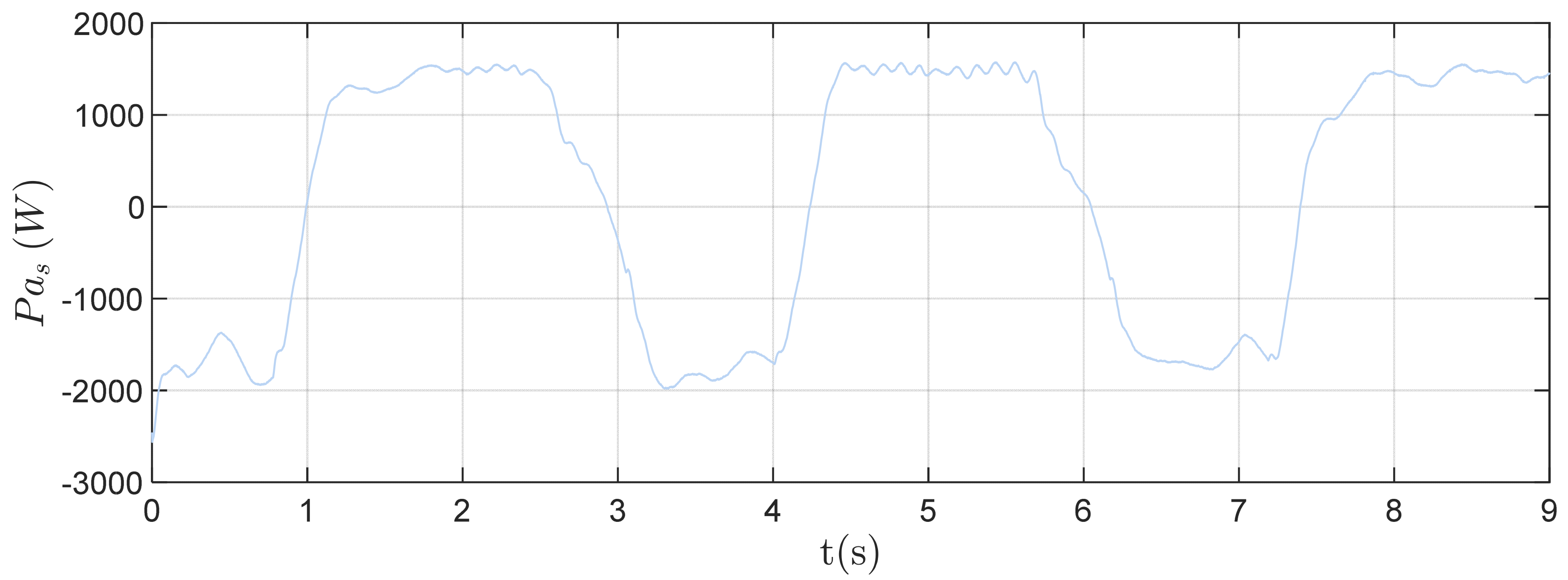
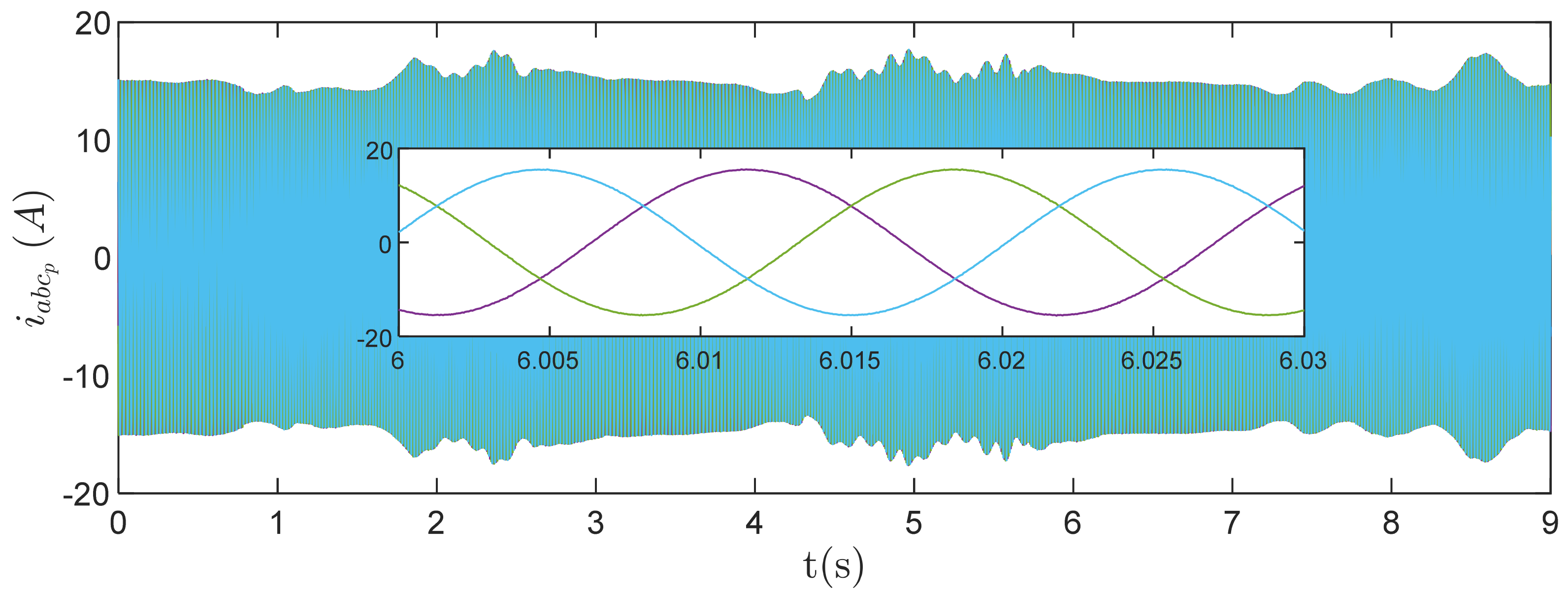
6. GPR-PTC Simulation Results

This section presents the simulation results of an autonomous wind energy conversion system utilizing the proposed GPR-PTC. The machine employed in this system has a nominal power of 8 kW. The wind behavior was simulated to mimic its natural intermittent nature, and a variable profile representing this behavior is depicted in Figure 6. This system supplied power to a resistive load of 150 Ohm, with a voltage of 600 V, as shown in Figure 7.
In Figure 7, it can be observed that the voltage error remains below 0.4%, which is considered a satisfactory result.
Figure 8 illustrates the variation in the machine’s speed, denoted as ω r , over time. It also shows the estimated speed value, denoted as ω ^ r   , and the speed reference, denoted as ω r . It can be observed that the speed value is accurately calculated and the estimation error remains below 0.5% (as shown in Figure 9). Furthermore, due to the effective speed regulation, the energy efficiency is consistently maintained at its nominal value of 0.438 (as depicted in Figure 10). These results highlight the efficiency and effectiveness of the GPR estimator utilized in this system.
Figure 11 demonstrates the power consumed by the load. Despite the fluctuations in the wind conditions, the load consistently consumed 3 kW with a maximum error of 0.8%, primarily due to the presence of a storage system. This storage system enables the storage of excess energy and compensates for any energy deficiency, as illustrated in Figure 12.
Figure 13 illustrates the variation in the stator flux. This flux is maintained at a nominal value of 1.2 Wb for speeds equal to or less than 307 rad/s. To prevent magnetic circuit saturation at higher speeds, a defluxion process was performed, as depicted in Figure 14. The maximum error in flow estimation is approximately 1.6 × 10⁻³%, indicating high accuracy.
Figure 15 illustrates the electromagnetic torque values of the ADSIG system. Specifically, T e s   represents the electromagnetic torque of the storage winding,   T e p represents the electromagnetic torque of the power winding, and T e represents the overall torque of the machine. Notably, the torque value remains negative throughout and does not change signs, indicating that the machine operated in generator mode. This behavior persisted even when the battery supplied energy. The reason behind this is that the energy delivered by the storage winding was directly transferred to the power winding, which was operating in transformer mode. Additionally, there was complete decoupling of the rotor, with no energy transfer from the storage winding to the squirrel cage.
Figure 16, Figure 17 and Figure 18 depict the values of the stator currents for the storage winding, power winding, and rotor currents, respectively. Based on these figures, it can be observed that the currents exhibit minimal harmonics and remain unaffected by the estimation error.

7. Conclusions

This research was dedicated to the implementation of speed-sensorless PTC in an autonomous wind power system that could effectively adapt to parametric variations. The utilization of a GPR-supervised learning algorithm as a speed and flux estimator proved to be a promising approach. The GPR algorithm was enhanced through the application of the gray box technique and further optimized using HBO. The latter part of this paper focuses on the successful integration of the trained GPR estimator into the studied system. The proposed intelligent GPR-PTC solution offers a robust and reliable approach to dealing with parametric variation, with the estimation errors of the speed and flux estimators having remained within an acceptable range of 0.5% (1.6 × 10⁻³%). Moreover, the control system showcased good energy efficiency, with a minimal drop of only 0.017% from its nominal value, resulting in cost-effectiveness. Furthermore, the load received a voltage of 600 V with a maximum error of 0.41%, indicating highly satisfactory performance. Moving forward, potential perspectives for this study include experimental validation of the proposed control system, exploration of alternative supervised learning algorithms and optimization techniques specifically tailored for this system, and consideration of additional constraints and larger training databases for real-world applications. The primary research challenge ahead lies in finding effective methods to reduce the size of the required training database.

Author Contributions

Conceptualization, writing—original draft preparation, software, Y.H.; validation, formal analysis, investigation and writing—review and editing, D.A., H.A., M.G.M.A. and T.S.U.; methodology, resources, data curation, visualization, Y.H., D.A., H.A., M.G.M.A. and T.S.U.; supervision and project administration, H.A. and T.S.U.; funding acquisition, T.S.U. All authors have read and agreed to the published version of the manuscript.

Funding

This research received no external funding.

Data Availability Statement

Not applicable.

Acknowledgments

We thank the DGRSDT of Algeria for providing the necessary subventions to our laboratory.

Conflicts of Interest

The authors declare no conflict of interest.

References

  1. Gielen, D.; Boshell, F.; Saygin, D.; Bazilian, M.D.; Wagner, N.; Gorini, R. The role of renewable energy in the global energy transformation. Energy Strategy Rev. 2019, 24, 38–50. [Google Scholar] [CrossRef]
  2. Nadeem, F.; Aftab, M.A.; Hussain, S.S.; Ali, I.; Tiwari, P.K.; Goswami, A.K.; Ustun, T.S. Virtual Power Plant Management in Smart Grids with XMPP Based IEC 61850 Communication. Energies 2019, 12, 2398. [Google Scholar] [CrossRef] [Green Version]
  3. Das, A.; Dawn, S.; Gope, S.; Ustun, T.S. A Strategy for System Risk Mitigation Using FACTS Devices in a Wind Incorporated Competitive Power System. Sustainability 2022, 14, 8069. [Google Scholar] [CrossRef]
  4. Singh, N.K.; Koley, C.; Gope, S.; Dawn, S.; Ustun, T.S. An Economic Risk Analysis in Wind and Pumped Hydro Energy Storage Integrated Power System Using Meta-Heuristic Algorithm. Sustainability 2021, 13, 13542. [Google Scholar] [CrossRef]
  5. Mousavi, S.M.G. An autonomous hybrid energy system of wind/tidal/microturbine/battery storage. Int. J. Electr. Power Energy Syst. 2012, 43, 1144–1154. [Google Scholar] [CrossRef]
  6. Housseini, B.; Okou, A.F.; Beguenane, R. Robust Nonlinear Controller Design for On-Grid/Off-Grid Wind Energy Battery-Storage System. IEEE Trans. Smart Grid 2017, 9, 5588–5598. [Google Scholar] [CrossRef]
  7. Chowdhury, M.M.; Haque, M.; Aktarujjaman, M.; Negnevitsky, M.; Gargoom, A. Grid integration impacts and energy storage systems for wind energy applications—A review. In Proceedings of the 2011 IEEE Power and Energy Society General Meeting, Detroit, MI, USA, 24–28 July 2011; pp. 1–8. [Google Scholar]
  8. Hamitouche, K.; Chekkal, S.; Amimeur, H.; Aouzellag, D. A New Control Strategy of Dual Stator Induction Generator with Power Regulation. J. Eur. Des. Syst. Autom. 2020, 53, 469–478. [Google Scholar] [CrossRef]
  9. Wang, F.; Zhang, Z.; Mei, X.; Rodríguez, J.; Kennel, R. Advanced Control Strategies of Induction Machine: Field Oriented Control, Direct Torque Control and Model Predictive Control. Energies 2018, 11, 120. [Google Scholar] [CrossRef] [Green Version]
  10. Bounasla, N.; Barkat, S. Optimum Design of Fractional Order PIα Speed Controller for Predictive Direct Torque Control of a Sensorless Five-Phase Permanent Magnet Synchronous Machine (PMSM). J. Eur. Syst. Autom. 2020, 53, 437–449. [Google Scholar]
  11. Ayala, M.; Doval-Gandoy, J.; Rodas, J.; Gonzalez, O.; Gregor, R.; Rivera, M. A Novel Modulated Model Predictive Control Applied to Six-Phase Induction Motor Drives. IEEE Trans. Ind. Electron. 2021, 68, 3672–3682. [Google Scholar] [CrossRef]
  12. Basic, M.; Vukadinovic, D.; Grgic, I.; Bubalo, M. Speed-Sensorless Vector Control of an Induction Generator Including Stray Load and Iron Losses and Online Parameter Tuning. IEEE Trans. Energy Convers. 2019, 35, 724–732. [Google Scholar] [CrossRef]
  13. Kumar, R.; Das, S.; Syam, P.; Chattopadhyay, A.K. Review on model reference adaptive system for sensorless vector control of induction motor drives. IET Electr. Power Appl. 2015, 9, 496–511. [Google Scholar] [CrossRef]
  14. Benlaloui, I.; Drid, S.; Chrifi-Alaoui, L.; Ouriagli, M. Implementation of a New MRAS Speed Sensorless Vector Control of Induction Machine. IEEE Trans. Energy Convers. 2014, 30, 588–595. [Google Scholar] [CrossRef]
  15. Korzonek, M.; Tarchala, G.; Orlowska-Kowalska, T. A review on MRAS-type speed estimators for reliable and efficient induction motor drives. ISA Trans. 2019, 93, 1–13. [Google Scholar] [CrossRef]
  16. Aurora, C.; Ferrara, A. A sliding mode observer for sensorless induction motor speed regulation. Int. J. Syst. Sci. 2007, 38, 913–929. [Google Scholar] [CrossRef]
  17. Shtessel, Y.; Edwards, C.; Fridman, L.; Levant, A. Sliding Mode Control and Observation; Springer: New York, NY, USA, 2014. [Google Scholar]
  18. Di Gennaro, S.; Dominguez, J.R.; Meza, M.A. Sensorless High Order Sliding Mode Control of Induction Motors with Core Loss. IEEE Trans. Ind. Electron. 2013, 61, 2678–2689. [Google Scholar] [CrossRef]
  19. Amirouche, E.; Iffouzar, K.; Houari, A.; Ghedamsi, K.; Aouzellag, D. Improved control strategy of dual star permanent magnet synchronous generator based tidal turbine system using sensorless field oriented control and direct power control techniques. Energy Sources Part A Recovery Util. Environ. Eff. 2021, 1–22. [Google Scholar] [CrossRef]
  20. Amirouche, E.; Iffouzar, K.; Houari, A.; Ghedamsi, K.; Aouzellag, D. Improved Control Strategy of DS-PMSG Based Standalone Tidal Turbine System Using Sensorless Field Oriented Control. Math. Model. Eng. Probl. 2021, 8, 293–301. [Google Scholar]
  21. Habibullah, M.; Lu, D.D.-C. A Speed-Sensorless FS-PTC of Induction Motors Using Extended Kalman Filters. IEEE Trans. Ind. Electron. 2015, 62, 6765–6778. [Google Scholar] [CrossRef] [Green Version]
  22. Tanvir, A.A.; Merabet, A. Artificial Neural Network and Kalman Filter for Estimation and Control in Standalone Induction Generator Wind Energy DC Microgrid. Energies 2020, 13, 1743. [Google Scholar] [CrossRef] [Green Version]
  23. Ridhatullah, A.I.; Hang Tuah Surabaya University; Joret, A.; Karyatanti, I.D.P.; Ponniran, A.; Malaysia, U.T.H.O. Three-Phase Induction Motor Speed Estimation Using Recurrent Neural Network Structure. J. Electron. Volt. Appl. 2021, 2, 23–35. [Google Scholar] [CrossRef]
  24. Pintelas, E.; Livieris, I.E.; Pintelas, P. A Grey-Box Ensemble Model Exploiting Black-Box Accuracy and White-Box Intrinsic Interpretability. Algorithms 2020, 13, 17. [Google Scholar] [CrossRef] [Green Version]
  25. Ufnalski, B.; Grzesiak, L.M. Selected Methods in Angular Rotor Speed Estimation for Induction Motor Drives. In Proceedings of the EUROCON 2007—The International Conference on “Computer as a Tool”, Warsaw, Poland, 9–12 September 2007; pp. 1764–1771. [Google Scholar]
  26. Yu, T.; Zhu, H. Hyper-Parameter Optimization: A Review of Algorithms and Applications. arXiv 2020, arXiv:2003.05689. [Google Scholar]
  27. Turner, R.; Eriksson, D.; McCourt, M.; Kiili, J.; Laaksonen, E.; Xu, Z.; Guyon, I. Bayesian Optimization is Superior to Random Search for Machine Learning Hyperparameter Tuning: Analysis of the Black-Box Optimization Challenge 2020. arXiv 2021, arXiv:2104.10201. [Google Scholar]
  28. Goguelin, S.; Dhokia, V.; Flynn, J.M. Bayesian optimisation of part orientation in additive manufacturing. Int. J. Comput. Integr. Manuf. 2021, 34, 1263–1284. [Google Scholar] [CrossRef]
  29. Shintani, K.; Fujimoto, T.; Okamoto, M.; Abe, A.; Yamamoto, Y. Surrogate modeling of waveform response using singular value decomposition and Bayesian optimization. J. Adv. Mech. Des. Syst. Manuf. 2021, 15, 20-00169. [Google Scholar] [CrossRef]
  30. Cai, D.; Liu, W.; Ji, L.; Shi, D. Bayesian optimization assisted meal bolus decision based on Gaussian processes learning and risk-sensitive control. Control Eng. Pract. 2021, 114, 104881. [Google Scholar] [CrossRef]
  31. Meldgaard, S.A.; Kolsbjerg, E.L.; Hammer, B. Machine learning enhanced global optimization by clustering local environments to enable bundled atomic energies. J. Chem. Phys. 2018, 149, 134104. [Google Scholar] [CrossRef] [Green Version]
  32. Brochu, E.; Brochu, T.; Freitas, N. A Bayesian interactive optimization approach to procedural animation design. In Proceedings of the SCA ‘10: Proceedings of the 2010 ACM SIGGRAPH/Eurographics Symposium on Computer Animation, Madrid, Spain, 2–4 July 2010; pp. 103–112. [Google Scholar]
  33. Lizotte, D.; Wang, T.; Bowling, M.; Schuurmans, D. Automatic gait optimization with Gaussian process regression. Int. Jt. Conf. Artif. Intell. 2007, 7, 944–949. [Google Scholar]
  34. Martinez-Cantin, R.; de Freitas, N.; Doucet, A.; Castellanos, J. Active Policy Learning for Robot Planning and Exploration under Uncertainty. In Robotics; The MIT Press: Cambridge, MA, USA, 2008; Volume 3, pp. 321–328. [Google Scholar] [CrossRef]
  35. Perdikaris, P.; Karniadakis, G.E. Model inversion via multi-fidelity Bayesian optimization: A new paradigm for parameter estimation in haemodynamics, and beyond. J. R. Soc. Interface 2016, 13, 20151107. [Google Scholar] [CrossRef] [Green Version]
  36. Galuzzi, B.G.; Perego, R.; Candelieri, A.; Archetti, F. Bayesian Optimization for Full Waveform Inversion. In AIRO Springer Series; Springer: Berlin/Heidelberg, Germany, 2018; Volume 1, pp. 257–264. [Google Scholar] [CrossRef] [Green Version]
  37. Marchant, R.; Ramos, F. Bayesian optimisation for Intelligent Environmental Monitoring. In Proceedings of the 2012 IEEE/RSJ International Conference on Intelligent Robots and Systems, Vilamoura-Algarve, Portugal, 7–12 October 2012; pp. 2242–2249. [Google Scholar]
  38. Wang, Z.; Shakibi, B.; Jin, L.; de Freitas, N. Bayesian Multi-Scale Optimistic Optimization. J. Mach. Learn. Res. 2014, 33, 1005–1014. [Google Scholar]
  39. Wang, Z.; Zoghiy, M.; Hutterz, F.; Matheson, D.; De Freitas, N. Bayesian optimization in high dimensions via random embeddings. Int. Jt. Conf. Artif. Intell. 2013, 1778–1784. [Google Scholar]
  40. Swersky, K.; Snoek, J.; Adams, R.P. Multi-task Bayesian optimization. Adv. Neural Inf. Process. Syst. 2013, 26, 1–9. [Google Scholar]
  41. Thornton, C.; Hutter, F.; Hoos, H.H.; Leyton-Brown, K. Auto-WEKA. In Proceedings of the 19th ACM SIGKDD International Conference on Knowledge Discovery and Data Mining, Chicago, IL, USA, 11–14 August 2013; Volume Part F1288, pp. 847–855. [Google Scholar]
  42. Srinivas, N.; Krause, A.; Kakade, S.; Seeger, M. Gaussian process optimization in the bandit setting: No regret and experimental design. In Proceedings of the 27th International Conference on International Conference on Machine Learning, Haifa, Israel, 21–24 June 2010; pp. 1015–1022. [Google Scholar]
  43. Mahendran, N.; Wang, Z.; Hamze, F.; De Freitas, N. Adaptive MCMC with Bayesian optimization. J. Mach. Learn. Res. 2012, 22, 751–760. [Google Scholar]
  44. Azimi, J.; Jalali, A.; Fern, X.Z. Hybrid batch bayesian optimization. In Proceedings of the 29th International Conference on Machine Learning ICML, Edinburgh, Scotland, 27 June–3 July 2012; 2, pp. 1215–1222. [Google Scholar]
  45. Brochu, E.; Cora, V.M.; de Freitas, N. A Tutorial on Bayesian Optimization of Expensive Cost Functions, with Application to Active User Modeling and Hierarchical Reinforcement Learning. arXiv 2010, arXiv:1012.2599. [Google Scholar]
  46. Benakcha, M.; Benalia, L.; Tourqui, D.E.; Benakcha, A. Backstepping control of dual stator induction generator used in wind energy conversion system. Int. J. Renew. Energy Res. 2018, 8, 384–395. [Google Scholar]
  47. Benakcha, M.; Benalia, L.; Ameur, F.; Tourqui, D.E. Control of dual stator induction generator integrated in wind energy conversion system. J. Energy Syst. 2017, 1, 21–31. [Google Scholar] [CrossRef] [Green Version]
  48. Amimeur, H.; Abdessemed, R.; Aouzellag, D.; Merabet, E.; Hamoudi, F. Modeling and Analysis of Dual-Stator Windings Self-Excited Induction Generator. J. Electr. Eng. 2015, 6, 1–6. [Google Scholar]
  49. Abdessemed, R.; Bendjeddou, Y.; Merabet, E. Improved field oriented control for stand alone dual star induction generator used in wind energy conversion. Eng. Rev. 2020, 40, 34–46. [Google Scholar] [CrossRef] [Green Version]
  50. Rasmussen, C.E.; Nickisch, H. Gaussian processes for machine learning (GPML) toolbox. J. Mach. Learn. Res. 2010, 11, 3011–3015. [Google Scholar]
  51. Kocijan, J.; Ažman, K.; Grancharova, A. The concept for Gaussian process model based system identification toolbox. In Proceedings of the 2007 International Conference on Computer Systems and Technologies—CompSysTech ’07, Sofia, Bulgaria, 14–15 June 2007; Volume 285, p. 1. [Google Scholar]
  52. Rasmussen, C.E.; Williams, C.K.I. Gaussian Processes for Machine Learning, 3rd ed.; MIT Press: Cambridge, MA, USA, 2008. [Google Scholar] [CrossRef] [Green Version]
  53. Myren, S.; Lawrence, E. A comparison of Gaussian processes and neural networks for computer model emulation and calibration. Stat. Anal. Data Min. ASA Data Sci. J. 2021, 14, 606–623. [Google Scholar] [CrossRef]
  54. Galuzzi, B.G.; Giordani, I.; Candelieri, A.; Perego, R.; Archetti, F. Hyperparameter optimization for recommender systems through Bayesian optimization. Comput. Manag. Sci. 2020, 17, 495–515. [Google Scholar] [CrossRef]
  55. Hannan, M.A.; Abdolrasol, M.G.M.; Mohamed, R.; Al-Shetwi, A.Q.; Ker, P.J.; Begum, R.A.; Muttaqi, K.M. ANN-Based Binary Backtracking Search Algorithm for VPP Optimal Scheduling and Cost-Effective Evaluation. IEEE Trans. Ind. Appl. 2021, 57, 5603–5613. [Google Scholar] [CrossRef]
  56. Abdolrasol, M.G.M.; Hussain, S.M.S.; Ustun, T.S.; Sarker, M.R.; Hannan, M.A.; Mohamed, R.; Ali, J.A.; Mekhilef, S.; Milad, A. Artificial Neural Networks Based Optimization Techniques: A Review. Electronics 2021, 10, 2689. [Google Scholar] [CrossRef]
  57. Abdolrasol, M.G.M.; Mohamed, R.; Hannan, M.A.; Al-Shetwi, A.Q.; Mansor, M.; Blaabjerg, F. Artificial Neural Network Based Particle Swarm Optimization for Microgrid Optimal Energy Scheduling. IEEE Trans. Power Electron. 2021, 36, 12151–12157. [Google Scholar] [CrossRef]
  58. Ustun, T.S.; Hussain, S.M.S.; Ulutas, A.; Onen, A.; Roomi, M.M.; Mashima, D. Machine Learning-Based Intrusion Detection for Achieving Cybersecurity in Smart Grids Using IEC 61850 GOOSE Messages. Symmetry 2021, 13, 826. [Google Scholar] [CrossRef]
  59. Ustun, T.S.; Hussain, S.M.S.; Yavuz, L.; Onen, A. Artificial Intelligence Based Intrusion Detection System for IEC 61850 Sampled Values under Symmetric and Asymmetric Faults. IEEE Access 2021, 9, 56486–56495. [Google Scholar] [CrossRef]
Figure 1. ADSIG autonomous DC generating system.
Energies 16 04738 g001
Figure 2. Representations of some iterations of Algorithm 1.
Energies 16 04738 g002aEnergies 16 04738 g002b
Figure 3. Proposed control block diagram for GPR-PTC.
Energies 16 04738 g003
Figure 4. Mean Square Error hyperparameters of the (a) speed and (b) flux GPR estimators.
Energies 16 04738 g004
Figure 5. Showcase of the validation and test results of the GPR model with the best hyperparameters for the speed estimator (a,b) and the flux estimator (c,d).
Energies 16 04738 g005
Figure 6. Wind speed profile over a duration of 9 s.
Energies 16 04738 g006
Figure 7. DC link voltage profile over a duration of 9 s.
Energies 16 04738 g007
Figure 8. ADSIG rotor speed over a duration of 9 s.
Energies 16 04738 g008
Figure 9. Speed estimation error over a duration of 9 s.
Energies 16 04738 g009
Figure 10. Actual power coefficients over a duration of 9 s.
Energies 16 04738 g010
Figure 11. Showcase of the output power of the power winding over a duration of 9 s.
Energies 16 04738 g011
Figure 12. Showcase of the output power of the storage winding over a duration of 9 s.
Energies 16 04738 g012
Figure 13. The variation of the stator flux over 9 s.
Energies 16 04738 g013
Figure 14. The variation of the magnetizing inductance for 9 s.
Energies 16 04738 g014
Figure 15. The variations of the electromagnetic torques of the two stator windings for 9 s.
Energies 16 04738 g015
Figure 16. The currents of the storage winding over a duration of 9 s.
Energies 16 04738 g016
Figure 17. Showcase of the currents of the power winding over a duration of 9 s.
Energies 16 04738 g017
Figure 18. The behavior of the three-phase abc rotor currents over a duration of 9 s.
Energies 16 04738 g018
Table 1. Machine specifications and values.
SpecificationsValues
Resistance of a Stator Phase r 1 = r 2 = 1.9  
Resistance of a Rotor Phase (Star 1 and 2) r r = 2.1    
Self-Leakage Inductance of a Stator Phase (star 1 and 2) L l 1 = L l 2 = 0.0132   H
Self-Leakage Inductance of a Rotor Phase L l r = 0.0132   H
Mutual Leakage Inductance Between Stator and Rotor L l m = 0.011   H
Cyclical Inter-Saturation Inductance between Stator and Rotor L d q = 0   H
Nominal Speed (Synchronism) v n = 1500   tr / min
Moment of Inertia J = 0.038   kg . m 2
Table 2. Showcase of the performances of the speed estimators.
SpeedANNSVMELDTGPR
RMSE (Validation)
(Test)
0.99045
1.3321
3.6243
2.786
3.3403
3.1116
3.3611
2.9657
0.27658
0.27412
R2 (Validation)
(Test)
1.00
1.00
0.99
1.00
1.00
1.00
1.00
1.00
1.00
1.00
MSE (Validation)
(Test)
0.98099
1.7745
13.136
7.7621
11.158
9.6818
11.297
8.7956
0.076498
0.07514
MAE (Validation)
(Test)
0.71611
0.97354
2.143
1.8061
2.4024
2.3535
2.0371
1.8879
0.21719
0.21417
Prediction Speed (~obs/s)160,000100,00047,000130,0003300
Training Time (s)140.82223.740.25318.6762427.5
Table 3. Showcases of the performances of the flux estimators.
FluxANNSVMELDTGPR
RMSE (Validation) (Test)0.015035
0.012887
0.017103
0.016238
0.016529
0.014499
0.021983
0.020285
0.0052222
0.0050421
R2 (Validation Test)0.99
0.99
0.99
0.99
0.99
0.99
0.98
0.98
1.00
1.00
MSE (Validation)
(Test)
0.00022604
0.00016609
0.00029252
0.00026366
0.0002732
0.00021023
0.00048327
0.00041149
2.7271 × 10⁻⁵
2.5423 × 10⁻⁵
MAE (Validation)
(Test)
0.010463
0.0093419
0.012947
0.012361
0.0094641
0.0083299
0.010803
0.010395
0.0035783
0.0033773
Prediction Speed (~obs/s)95,000110,00042,00047,0005700
Training Time (s)338.42385.563.99936.9181022.6
Table 4. Gaussian Process Regression hyperparameters.
SpeedFlux
Sigma493.93260.043146
Basis FunctionConstantLinear
Kernel FunctionNon-isotropic rational
quadratic
Non-isotropic matern 5/2
StandardizedFalseFalse
Disclaimer/Publisher’s Note: The statements, opinions and data contained in all publications are solely those of the individual author(s) and contributor(s) and not of MDPI and/or the editor(s). MDPI and/or the editor(s) disclaim responsibility for any injury to people or property resulting from any ideas, methods, instructions or products referred to in the content.

