1. Introduction
Agreed climate targets can only be met through a radical reduction in greenhouse gas emissions. Energy-intensive industries are responsible for a significant share of these emissions. The economic pressure of reducing emissions requires companies to pursue cost-effective solutions. One way to reduce emissions cost-effectively is to connect hot and cold process streams. A heat exchanger network (HEN) enables heat exchange between process streams and thus reduces the energy demand for heating or cooling. The design of an HEN is a complex task due to the high combinatorics of numerous possible connections between streams. Based on the objective function, an optimal HEN can be determined by applying heat exchanger network synthesis (HENS).
The HEN design problem was first mentioned by Ten Broeck in 1944 [
1]. The first formal definition was published by Masso and Rudd in 1969 [
2]. All these approaches are sequential methods that decompose the HENS problem into a set of subproblems. Decomposition requires parameter estimation and iterative optimization, which is why the optimal solution is challenging to find. Fully simultaneous methods calculate the optimal utility consumption, stream matches and HEN configuration simultaneously [
3]. The first simultaneous HENS were published by Yuan et al. [
4] in 1989, Yee and Grossmann [
5] in 1990 and Ciric and Floudas [
3] in 1991. For a more detailed elaboration of the historical development, the papers by Furman and Nikolaos [
6] and Escobar and Trierweiler [
7] are recommended. The latter have shown in their work that Yee and Grossmann’s stage-wise superstructure formulation [
5] gives better results in terms of total annual cost (TAC) at lower computation times. Therefore, in this paper, we will build on this formulation. Further interesting approaches can be found in the work of Gu et al. [
8] and Zirngast et al. [
9]. In contrast to the traditional methods, the latter two address uncertainties in the stream definition.
In Yee and Grossmann’s formulation, two assumptions are made that may lead to sub-optimal HENs: First, implementing utilities is only possible with predefined inlet and outlet temperatures. This assumption is only reasonable where utilities condense a medium at a constant temperature and pressure. If only the sensitive heat in, for example, flue gas or cooling water is used, the temperatures to which the medium must be cooled or heated are of minor importance. Usually, there is a margin for utility temperatures in terms of regulatory and process requirements. Secondly, the utilities must always reach the set temperature in only one heat exchanger without stream splits. In contrast, hot and cold process streams can reach their set target temperature using multi-staged heat exchangers with stream splits. These two limitations inhibit the field application. Considering multi-stage utilities with variable temperatures is essential to optimally integrate the heat sink and source into the process. To run HENS without these assumptions, the Yee and Grossmann formulation has to be adapted.
Yee and Grossmann’s non-linear formulation belongs to the class of
-hard problems [
10]. Even with state-of-the-art computational power and solvers, the optimal heat integration of complex industrial processes cannot be calculated. Implementing utilities as streams with variable temperatures and flow capacities further increases the complexity of the optimization problem. Martelli et al. [
11], for example, proposed an MINLP model for complex utility handling using a two-stage algorithm. Moreover, it can never be guaranteed that the optimal solution has been found. Piecewise-linear approximation of the non-linear terms (mean logarithmic temperature difference (LMTD), heat exchanger areas, and energy balances) is necessary to find a global minimum within feasible computation time, even though the problem is still
-hard. Beck and Hofmann [
12] linearized the superstructure formulation and applied mixed-integer linear programming (MILP) to solve the problem. Compared to the non-linear model, they achieved better results in terms of TAC with shorter computation times.
Paper Organization
This paper presents a novel piecewise-linear implementation of utilities as multi-stage streams with stream splits, variable temperatures, and flow capacities. The methods in
Section 2 are divided into two main sections. First, all our essential adaptations of the superstructure formulation are presented in
Section 2.1. In
Section 2.2, the piecewise-linear approximation of the non-linear terms with hyperplanes and simplices and the transfer to MILP is shown.
Section 3 introduces three representative use cases from the literature and industrial problems. For each use case, either a cold utility or a cold and a hot utility is implemented as a stream with variable outlet temperature and heat capacity flow. A comparison is made for the results with and without variable utility definitions. We show that minor variations in the utility outlet temperature lead to a significant improvement in terms of TAC. We therefore conclude in
Section 4 that variable outlet temperatures and flow capacities allow the cost-optimal design of the necessary utilities.
2. Methods
2.1. Modification of the Superstructure
One way of realizing multi-stage utilities is to implement them as streams with stream splits. However, one consequence is that the flow capacity must be specified. If one degree of freedom is blocked by setting the flow capacity for the utility stream, the utilities may not necessarily provide the required energy for heating or cooling the streams. Introducing an additional variable for the flow capacity makes the optimization problem non-linear again. Implementing a variable outlet temperature requires another variable. Both variables are independent and form non-linear relationships, further increasing the complexity of the problem.
Referring to the stage-wise superstructure according to Yee and Grossmann [
5], cold (UC) and hot utilities (UH) can only be located at the end of the streams. The streams can exchange heat in
stages.
In this paper, we extend the formulation to implement hot and cold utilities as streams—hereafter referred to as utility streams (US). The objective function
where
and
minimizes the TAC of the heat exchanger network.
If the flow capacity and the outlet temperature are constant, Equation (
4) is used to constrain the utility heat loads.
If hot utility streams (HUS) and/or cold utility streams (CUS) are implemented, the utilities are no longer necessary and disabled with Equation (
5).
The heat exchange between utilities and streams always occurs at the stream ends in only one stage and without stream splits. This results in a total of
stages for heat exchange with other streams and the utility. Due to the disabled utilities, only
stages are available for the US heat exchange. Increasing the number of stages by one ensures that the same number of stages are available for heat exchange compared to the original superstructure formulation.
Blocking the stream heat exchange with Equation (
6) at the added stage secures the stream-to-stream heat exchange at the initial
stages.
The temperatures at position
and
in Equations (
7) and (
8) correspond to the inlet and outlet temperatures of the streams.
If at least two of the three variables on the right side are assigned a discrete value with Equations (
11), (
13) or (
14), the constraints of the stream-wise energy balance remain linear. If fewer values are set, the piecewise-linear approximation presented in
Section 2.2.3 is used.
The stage-wise energy balance can be constrained with Equation (
9). If the flow capacity
is not set to a predefined value with Equation (
11), the piecewise-linear approximation from
Section 2.2.3 is used.
The flow capacities are set to a specific value with Equation (
11). Otherwise,
F is bounded to the predefined range
with Equation (
12).
Constant inlet or outlet temperatures are set with Equations (
13) and (
14). Variable temperatures are constrained to a specified range for the inlet temperature
and the range for the outlet temperature
using Equations (
15) and (
16), respectively.
Note that, if stream inlet and outlet temperatures are defined in a specific range, the conditions
must always be fulfilled to obtain a feasible solution.
The following constraints are not affected by variable temperatures or flow capacities.
Monotonic decrease in temperature:
Bounds for temperature differences:
Non-negativity constraints:
2.2. Piecewise-Linear Approximation
To integrate the design of the utilities into the HENS and find a global optimum within a feasible computation time, piecewise-linear approximation is essential. For the sake of simplicity, a function with one primary curvature is called convex or concave accordingly. In contrast to the convex heat exchanger area of the streams and the concave heat exchanger surface of the utilities, the energy balance is neither convex nor concave. The energy balance is essentially a multiplication of two independent variables. The resulting saddle-shaped function can no longer be represented with sufficient accuracy by simple concave or convex approximations. Therefore, the following two methods for linear approximation are distinguished in this paper: Piecewise-linear approximation with hyperplanes and with simplices. Piecewise-linear approximation with hyperplanes is used for the convex function of the stream HEX area (see
Section 2.2.1) and the concave function of the utility HEX area (see
Section 2.2.2). Each hyperplane is defined linear function with coefficients
a, which specifies offset and slope. The coefficients
a are determined using a nonlinear optimization that minimizes the sum of squares error (SSE) between the linearized planes and the data points. Concave functions can be linearized in the same way by considering the identity
. The accuracy of the approximation can be adjusted by adding hyperplanes until a defined root-mean-square error (RMSE) is reached. In contrast to piecewise-linear approximation with simplices, only limited accuracy can be achieved for non-convex or non-concave approximations.
Convex or concave approximation with hyperplanes is only suitable for functions that curve in only one direction. In the natural sciences, however, problems often occur which require a multiplication of optimization variables. For example, the two-dimensional function
is saddle-shaped and cannot be approximated convexly or concavely with sufficient accuracy. By contrast, any continuous function can be approximated piecewise-linearly with simplices. In the two-dimensional set, for a grid with
w elements, the function
can be divided into triangles [
13]. The function
f can thus be approximated with piecewise functions linearly within the triangles. In this paper, the
union jack triangulation is used. This method requires a grid with the nodes of the triangles in its intersection. A non-linear optimization problem determines the grid points and the plane equations of the triangles by minimizing the SSE. Piecewise-linear approximation with simplices is used for the stream- and stage-wise energy balances (see
Section 2.2.3) and the LMTD (see
Section 2.2.4).
2.2.1. Stream Heat Exchanger Area
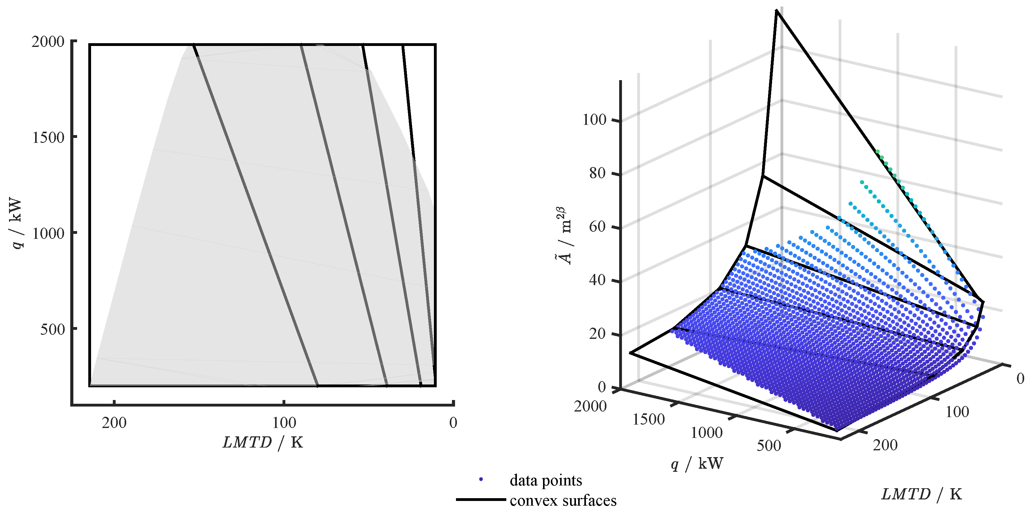
The reduced heat exchanger area
for a stream HEX is a convex function. Beck et al. formulate a linear optimization problem to constrain the independent variables
q and
to a physically feasible domain. The
hyperplanes of the two-dimensional function are defined with coefficients
such that
for each data point.
Figure 1 shows the reduced solution space with 2014 data points in a light gray and hyperplane approximation for two example streams. Within this example, we are able to achieve an RMSE of 1.26% using 5 hyperplanes. Above 22 hyperplanes, the RMSE of 1.16% does not change within the lsqnonlin solver’s step size tolerance of 10
−6.
2.2.2. Utility Heat Exchanger Area
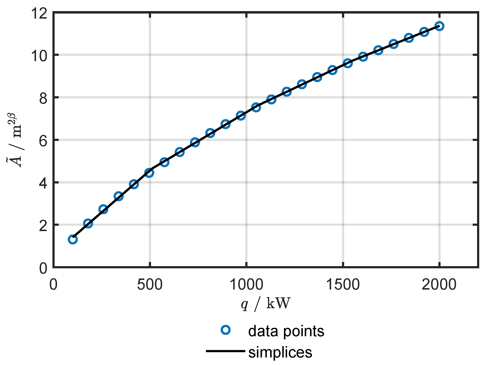
Since three out of four temperatures are fixed at the utility heat exchangers, the reduced heat exchanger area can be formulated as a function of the heat flow
q [
12]. The one-dimensional correlation of the reduced heat exchanger area for hot utilities
and cold utilities
is a concave function. Equations (
26) and (
27) are restricted to the physically solvable domain and represented by lines. The lines are thus represented as linear equations
for each plane and heat exchanger. The coefficients are determined by non-linear minimization of the SSE until an RMSE criterion is met.
Figure 2 shows the concave function of the reduced utility HEX area with 25 data points and the piecewise-linear approximation. With four lines, an RMSE of 0.38% can be achieved. In this case, an ideal linear approximation would be possible by interpolating the data points. In this case, the improved accuracy is out of proportion to the required binary variables, which unnecessarily increases the complexity and computation time of the optimization problem.
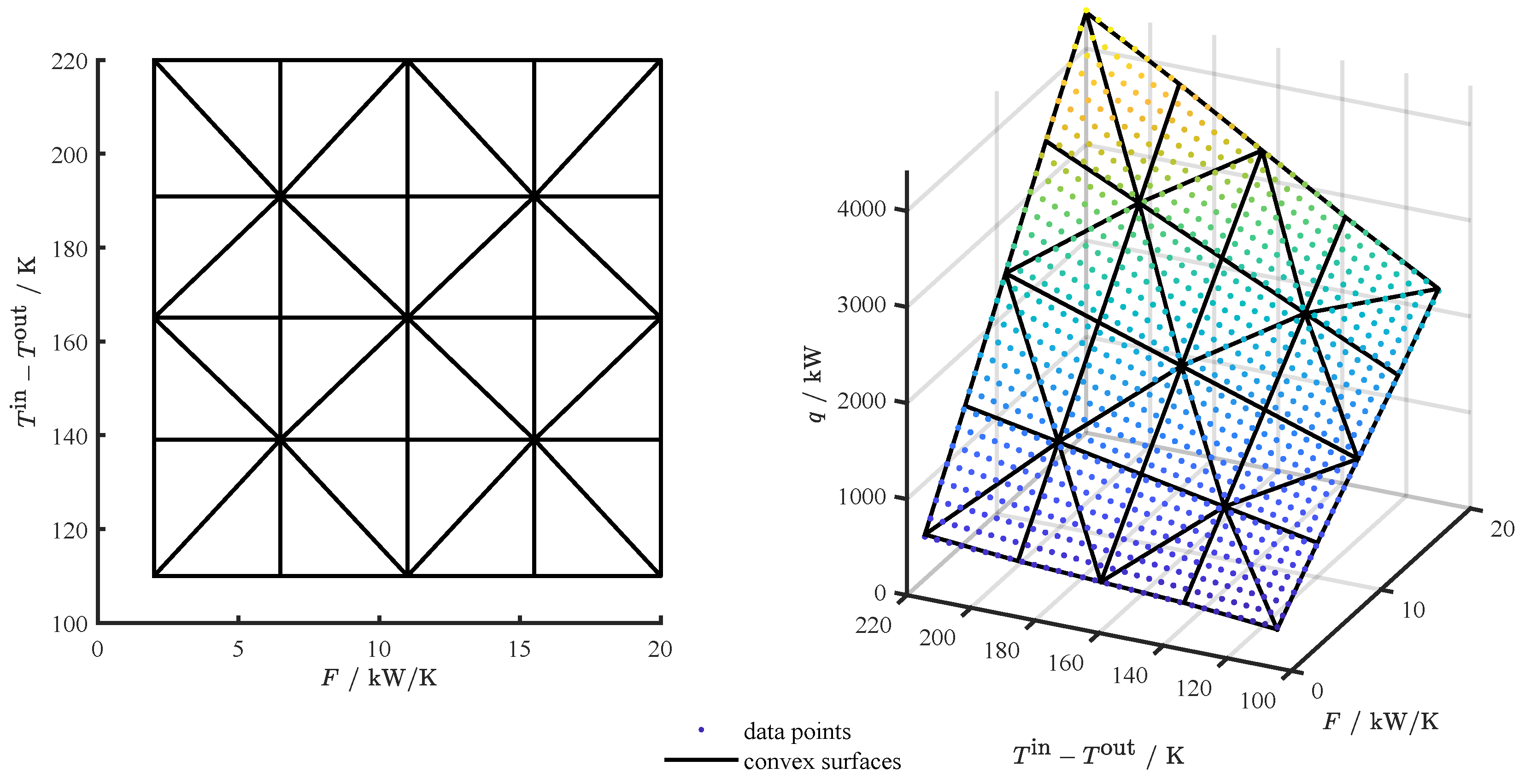
2.2.3. Energy Balances
The piecewise-linear approximation of the energy balances, Equations (
7)–(
10), is of central importance to implementing streams with variable inlet or outlet temperature and flow capacity.
Figure 3 shows the 900 data points and the piecewise-linear approximation with simplices of a streamwise-energy balance. The heat flow
q is plotted as a function of the flow capacity
F and the temperature difference
. The saddle-shaped function is approximated with 32 simplices on an equidistant 4 × 4 grid with an RMSE of 0.28%.
2.2.4. LMTD
The LMTD, according to Equation (
3), is concave and can be approximated with hyperplanes and simplices. Both methods require additional binary variables. The approximation with simplices offers considerable advantages in terms of the MILP translation. Significantly higher accuracies can be achieved with the same number of binary variables.
Figure 4 shows the piecewise-linear approximated LMTD with 900 data points on a 4 × 4 grid. In regions with larger curvature, more simplices are placed.
2.3. Translation to MILP
The translation to MILP should be carried out with as few auxiliary binary and continuous variables as possible. Thus, the minimization problem can be solved efficiently within a feasible timeframe.
The streams’ convex reduced HEX area is translated most easily to MILP. The hyperplanes shown in
Figure 1 can be translated to MILP with one inequality each and without additional binary variables, see [
12].
For all other functions, binary variables are necessary to translate the simplices into MILP. Vielma and Nemhauser [
13] developed a logarithmic approach to reduce the number of binary variables. A grid with
w elements in an
n-dimensional space, where
w is a power of two, is composed of
simplices. The
T simplices can be translated to MILP highly efficiently with
binary variables and
continuous variables. The piecewise-linear approximations based on simplices presented in the previous sections are all on a grid with
elements in each dimension. The one-dimensional approximation of the utility HEX area in
Figure 2 is modeled with four simplices. Thus, two binary variables and four additional constraints are used to translate the correlation to MILP. On the other hand, the widely used SOS2 approach would require four binary variables. The approximation of the two-dimensional correlations for the streams HEX area, energy balance, and LMTD is composed of 32 simplices. These can be translated to MILP with five binary variables and ten additional constraints each. Due to the small number of binary variables combined with the high accuracy of the approximation, non-linear correlations can be approximated highly efficiently and modern MILP solvers can calculate a global optimum in feasible computing time.
Since not all approximations reach the value
, the functions are toggled with binary variables and a big-M approach. The hyperplane approximation’s maximum value always occurs in the corner of the domain. Accordingly, the big-M value is chosen. By choosing the smallest possible big-M value, the problem remains tight and the stability of the numerical solving algorithms is improved because the feasible region of the LP relaxation is not unnecessarily expanded [
14].
3. Case Studies & Results
This paper examines whether it is beneficial in terms of TAC to implement utilities as multi-stage streams with stream splits and variable outlet temperature and flow capacity. Furthermore, the influence of the utility outlet temperature on the TAC is studied. For this purpose, in each of the three representative case studies (CS), all utilities that only use sensible heat are implemented as streams. To ensure comparability with the results from the literature, we use only cost factors proportional to the utility heat flow.
Depending on the utilities, the following cases were considered:
- base
For each case study, the base case is used to compare the results with literature values and to validate the optimization framework.
- var UC
A cold utility with variable outlet temperature and flow capacity is implemented when only the sensible heat of a medium such as water or thermal oil is used for cooling.
- var UC & UH
A hot and cold utility with variable outlet temperature and flow capacity is implemented when only the sensible heat is used for both cooling and heating.
3.1. Piecwise-Linear Approximation & Implementation
Planes were added to the linear models of the stream HEX area until the RMSE was below 1.0%. To limit the number of binaries used to transfer the simplices to MILP, the approximation of the utility HEX area, energy balances, and LMTD were calculated on a 4 × 4 grid with 32 simplices. The is below 0.5% for all models.
All optimization problems in this paper were modeled using Yalmip R20210331 [
15] in Matlab R2022b [
16]. All problems were solved using Gurobi 9.5.2 on a 128-core system (AMD EPYC 7702P) with 256 GB of RAM.
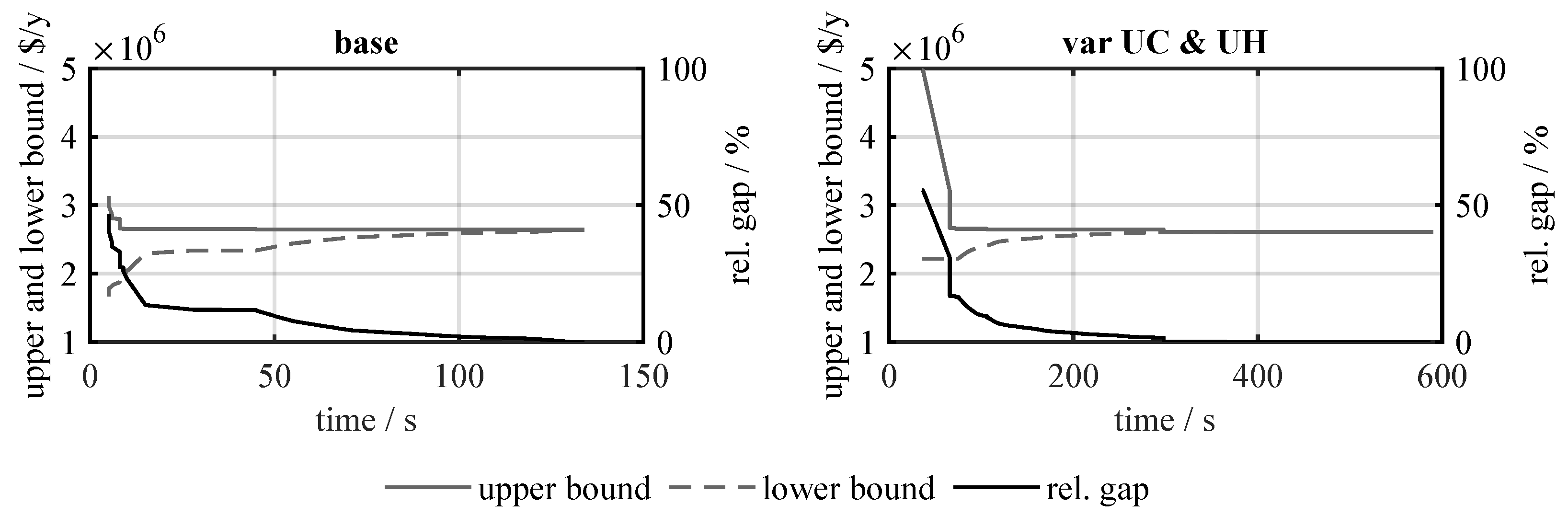
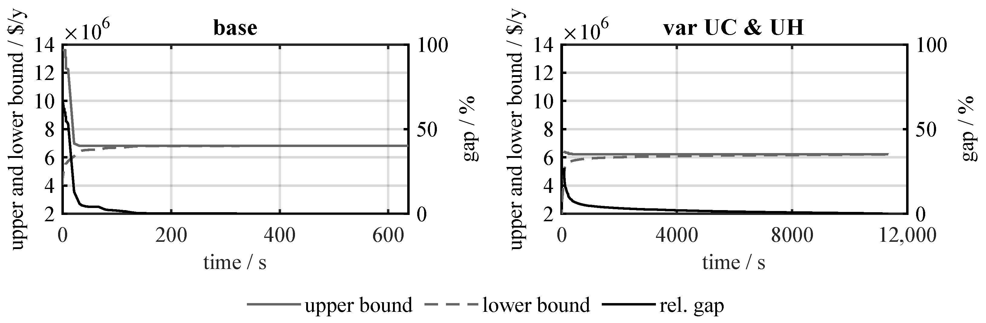
Each optimization problem was solved three times. The solution with the lowest computation time is presented. The convergence behavior over time is shown in
Appendix A with its characteristic values, relative gap, upper and lower objective bounds. The relative gap is defined as the gap between the best feasible solution objective and the best bound. The calculations are terminated if the relative gap is smaller or equal than the tolerance of the MIP solver. The default value is 0.01%.
3.2. Case Study 1
The first case study was presented by Ahmad [
17] and is composed of two hot and two cold streams. The stream data is listed in
Table 1. Since the latent heat of steam is used as the hot utility, the outlet temperature of the steam cannot be adjusted without changing the steam parameters. Accordingly, no HUS is implemented. Since only the sensible heat of the cooling water is used, the cold utility is implemented as CUS. The CUS stream definition is marked with the superscript v. The parentheses specify the range of permissible values for the outlet temperature and the flow capacity.
Results
The number of variables, the computation time, and the relative gap for CS1 can be seen in
Table 2. The number of binary variables increases significantly with one implemented CUS from 120 to 376. Therefore, the computation time for the var UC case of 22.79 S is nearly ten times that of the base case with 2.30 S.
To validate the developed framework, the base case is compared with three references from the literature. The results are summarized in
Table 3. The stream plots of the resulting HENs are shown in
Appendix B. The optimal HENs of Ahmad [
17], Nielsen et al. [
18], and Khorasany and Fesanghary [
19] were calculated without using stream splits. Khorasany and Fesanghary [
19] used a two-level approach with a harmony search algorithm and sequential quadratic programming to determine the best known literature value for minimum TAC of 1.1895 × 10
4 $/y. In contrast to the literature values, we used three stages instead of four and allowed for stream splits.
We were able to find a solution for the base case with 1.1792 × 10
4 $/y of TAC. In terms of TAC, the calculated solution is 0.87% cheaper than the best literature value from Khorasany and Fesanghary [
19]. Since both the values of the TAC and the heat loads show only minor deviations, it can be assumed that the framework presented in this paper provides reliable results.
Implementing the CUS, we can find a solution with 1.08% lower TAC than the best literature value provided by Khorasany and Fesanghary [
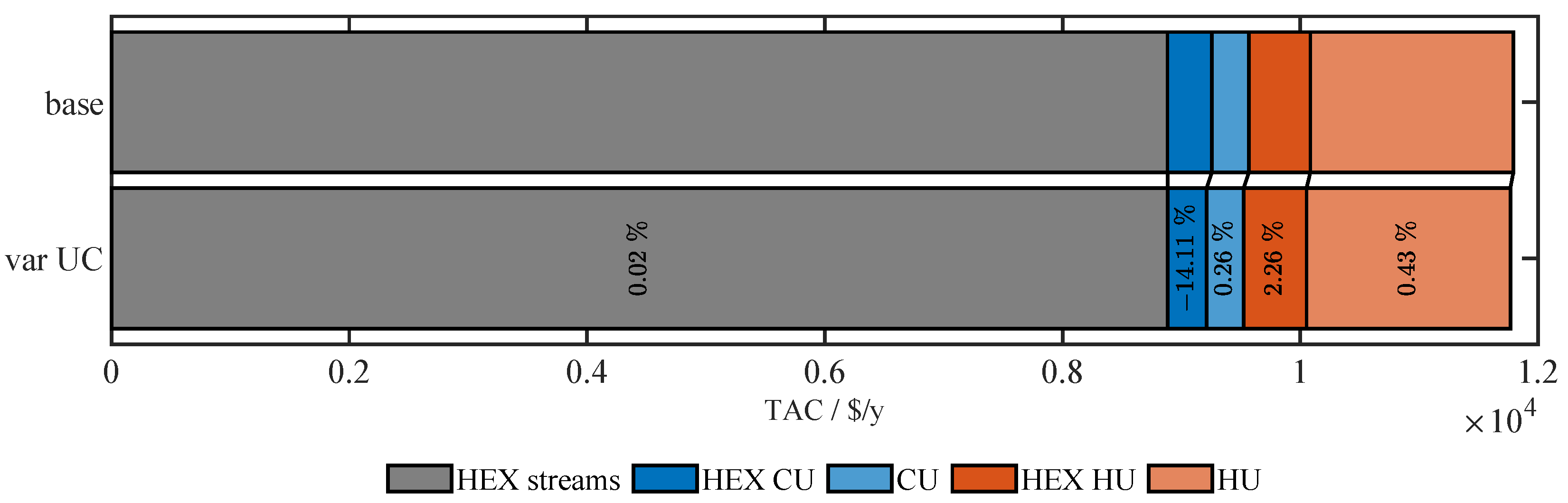
19]. Compared to the base case, 0.29% can be saved. As seen from the cost structure in
Figure 5, the energy costs of the hot and cold utilities slightly increase compared to the base case. The main cost-saving results from the smaller heat exchanger area at the cold utility. The stream matches of the two resulting HENs are both identical; see
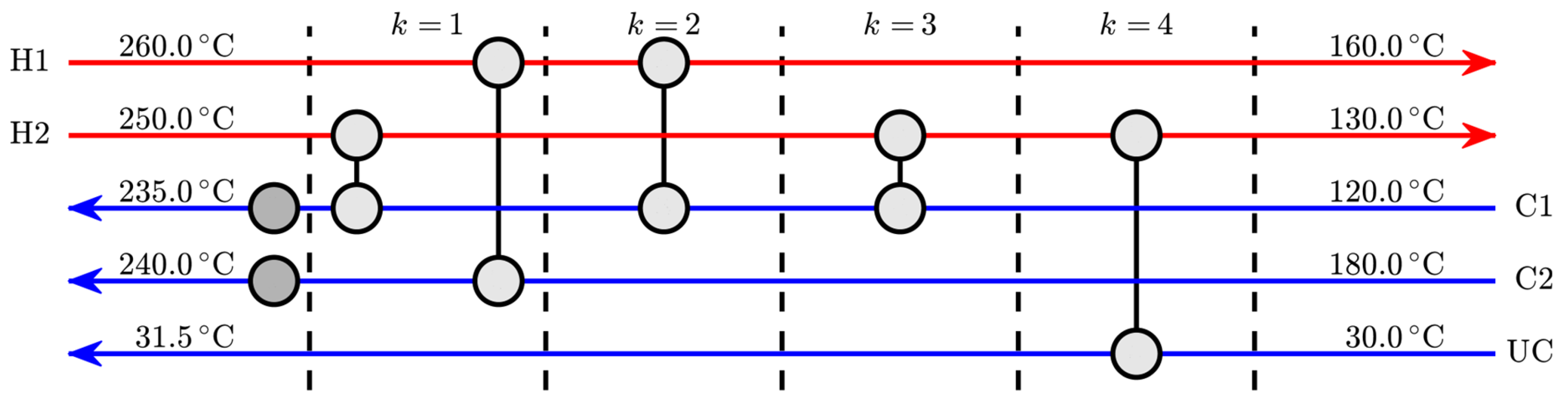
Appendix B. Accordingly, the heat exchanger costs of the streams are almost identical. The outlet temperature of the CUS of 31.5 °C is close to the lower valid range of 31 °C. In contrast to the CU of the base case, the CUS temperature difference between the inlet and the outlet is reduced from 15 K to 1.5 K. The reduced temperature difference results in a large LMTD, which in turn results in a smaller and less expensive HEX area.
3.3. Case Study 2
In the second case study, a frequently discussed aromatics plant in the literature is considered. The stream data provided by Linnhoff and Ahmad [
20] is given in
Table 4. In this case study, thermal oil is used as hot utility. Since only the sensible heat of the oil is used, the outlet temperature can be adjusted and the hot utility is implemented as HUS. The cold utility uses the sensible heat of cooling water and is therefore implemented as CUS. In contrast to CS1, two streams with variable outlet temperatures and flow capacities are implemented.
Results
As can be seen from
Table 5, the number of binary variables for the var UC and UH case has more than tripled compared to the base case. Due to the higher complexity, the computation time also increases from 133.95 s to 590.12 s.
Table 6 lists a comparison of the calculated values with data from the literature. Linnhoff and Ahmad [
20] used the pinch design method and the driving force plot to obtain a HEN with 2.9300 × 10
6 $/y of TAC. Through evolution and continuous optimization of the exchanger duties, they were able to obtain TAC of 2.8900 × 10
6 $/y. In both calculations, the minimum temperature difference at the hot utility of 26 °C; was violated, causing the outlet temperature of the thermal oil to be higher than 250 °C. Fieg et al. [
21] corrected this by calculating the hot utility costs proportional to the thermal oil mass flow rate as a function of the outlet temperature. The TAC of 2.9300 × 10
6 $/y was corrected to 2.9920 × 10
6 $/y, and of 2.8900 × 10
6 $/y to 3.0250 × 10
6 $/y, respectively. Fieg et al. [
21] also calculated an even cheaper solution with 2.9223 × 10
6 $/y of TAC using a hybrid genetic algorithm (GA). Lewin [
22] used a GA to find several solutions using different parameters of the algorithm. Despite an assumed minimum temperature difference of 10 °C, the outlet temperature of the hot utility was raised without considering mass-flow-dependent costs. The best solution has a TAC of 2.9360 × 10
6 $/y. Zhu et al. [
23] found the most expensive solution so far with TAC of 2.9700 × 10
6 $/y through a two-step procedure using heuristics and nonlinear optimization. The optimizations performed in the literature enable a HEN with three stages and stream splits. In order to be able to compare our results with the literature, we assume, on the one hand, that the costs are proportional to the heat flow. On the other hand, we use a lower bound for the minimum temperature difference of 1 °C.
For the base case, TAC of 2.9114 × 10
6 $/y could be calculated using only two stages and stream splits. Compared to the best literature value from Linnhoff and Ahmad [
20], this solution is 0.74% more expensive. Compared to the worst literature value from Zhu et al. [
23], however, it is 2.01% cheaper.
The TAC can be reduced to 2.8526 × 10
6 $/y by implementing a CUS and a HUS. Compared to the best literature value provided by Linnhoff and Ahmad [
20], the solution of the var UC and UH case is 1.30% cheaper. The heat loads differ only slightly in both cases. The stream plots are shown in
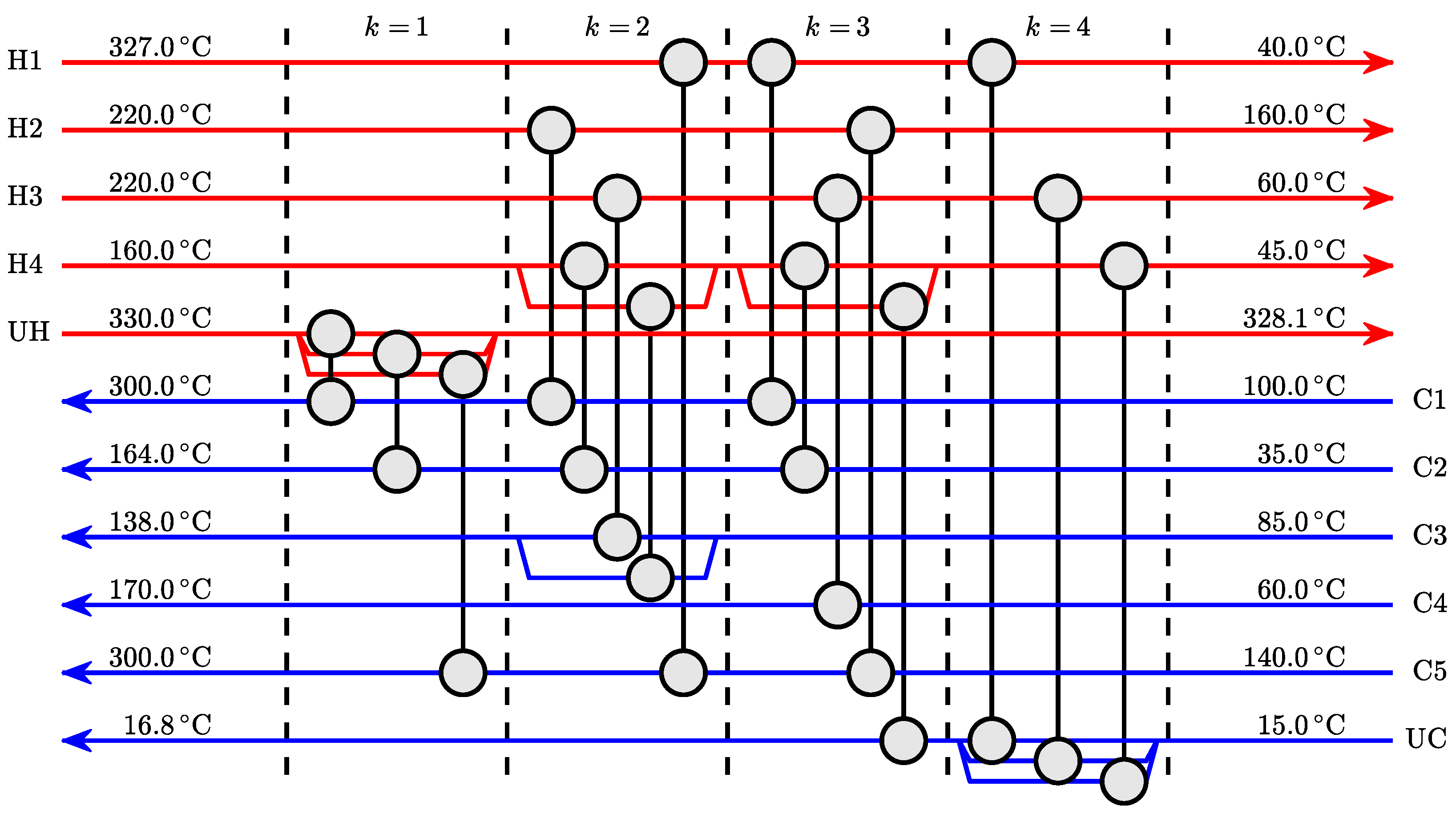
Appendix B. The stream matches of the hot and cold streams are identical in both cases. The hot utility is used on the cold streams C1, C2, and C5 in both cases. The outlet temperature of the hot utility increases from 250.0 °C to 328.1 °C. The cold utility is used in the base case and the var UC and UH case on streams H1, H3, and H4. In the var UC and UH case, the cold utility is used a second time on stream H4. In this case, the CUS exchanges heat at two stages with the hot streams. The outlet temperature of the cooling water decreases from 30.0 °C to 16.8 °C. Analogous to CS1, based on the cost structure and its relative change to the base case costs in
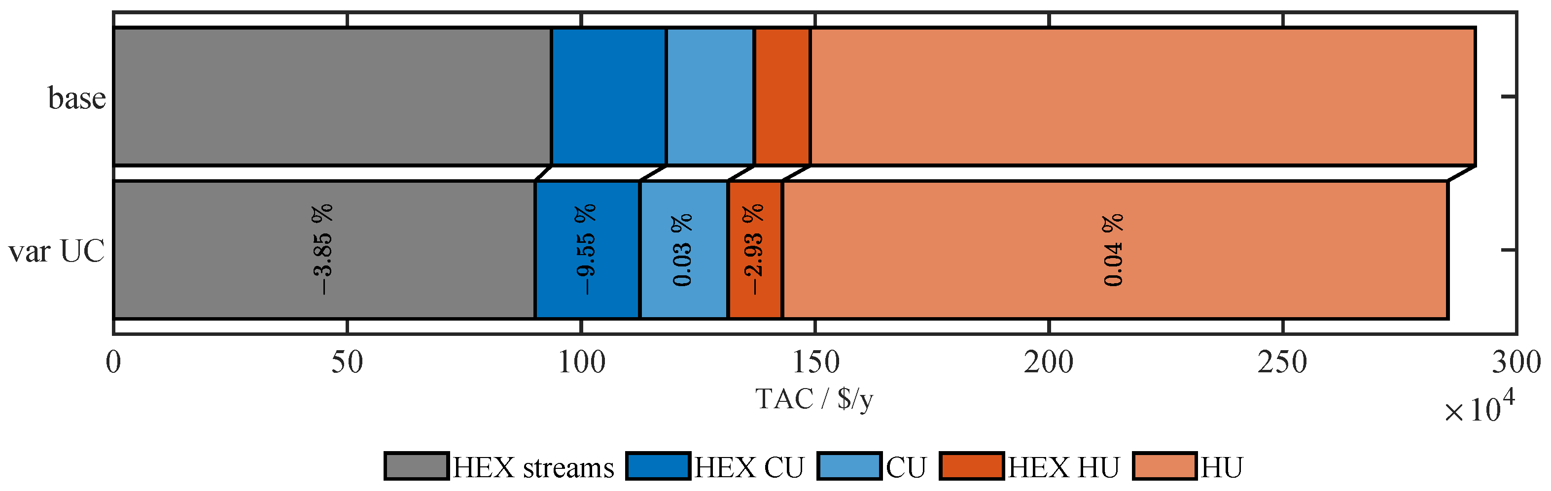
Figure 6, the most significant cost reduction can be found in the heat exchanger areas for hot and cold utilities.
3.4. Case Study 3
The third case study is the Bandar Imam aromatic plant on the northwestern coast of the Persian Gulf. The real-world problem includes six hot and ten cold streams. The stream data was provided by Khorasany and Fesanghary [
19] and is listed in
Table 7. Khorasany and Fesanghary [
19] probably made a conversion error from °C to K for the cold utility [
24,
25,
26,
27]. Since cooling water is used as cold utility, it is implemented as CUS. In this case, two hot utilties are available: flue gas (UH
1) and steam (UH
2). The flue gas utility is implemented as HUS. The steam utility is implemented as a conventional utility without variable temperatures and flow capacity.
Results
Table 8 lists the number of variables, computation time, and relative gap. Both cases were optimally solved within the defined MIP gap. Due to the high complexity of the var UC and UH case, the computation time is the highest with 11,335.64 s (3.15 h).
Table 9 compares the TAC and heat loads of the existing power plant with those from literature and those calculated in this paper. Khorasany and Fesanghary [
19] used the same two-level approach as for CS1 to optimize the HEN of the aromatic plant. The optimized HEN with TAC of 7.4357 × 10
6 $/y results in a cost savings of 16.00% compared to the existing plant. Feyli et al. [
25] found TAC of 7.1285 × 10
6 $/y using GA and a quasi-linear programming method. The HEN has eight stages and no stream splits. Aguitoni et al. [
28] found a slight improvement in TAC. Here, the discrete variables were optimized with a GA and the heat loads on the streams, and the stream split fractions were optimized with the help of differential evolution. The resulting HEN has three stages with stream splits. Pavão et al. followed a two-level approach in [
24,
29], handling the binary variables with simulated annealing. The continuous variables are optimized using a rocket fireworks approach. In [
29], the super-structure formulation was adapted, allowing intermediate placement of utilities. In [
24], sub-stages, sub-splits, and cross-flows are additionally enabled. Nair and Karimi [
26] used a stageless superstructure formulation with stream splits to optimize the TAC. Here, MILP relaxations are solved to find a lower bound on the TAC. Constraining the configurations and solving the nonlinear problem yield to an upper bound on the TAC. The lowest TAC to date of 6.6647 × 10
6 $/y could be determined by Liu et al. [
30] using a GA approach with intermediate utility placement.
In this paper, we obtained TAC of 6.7451 × 10
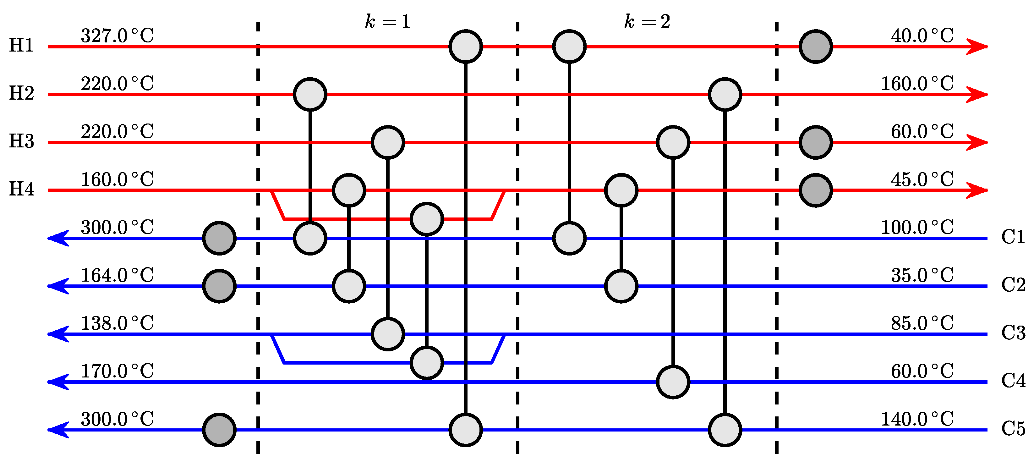
6 $/y for the base case with two stages and stream splits. The stream plots are shown in
Appendix B. Like most solutions from the literature, the second hot utility (steam) is not used. Compared to the best literature value of Liu et al. [
30], this solution is 1.19% more expensive. However, our solution is 31.30% cheaper than the existing plant.
In the var UC and UH case, the TAC can be reduced to 6.3297 × 10
6 $/y through the implementation of a HUS and a CUS. Thus, this solution is 5.37% cheaper than the best solution provided by Liu et al. [
30]. Compared to the existing plant, the TAC can be reduced by 40.49%. In the base and var UC and UH case, the second utility (steam) is not used. The HEN configuration of the two cases differs only in the first and fifth hot stream; see
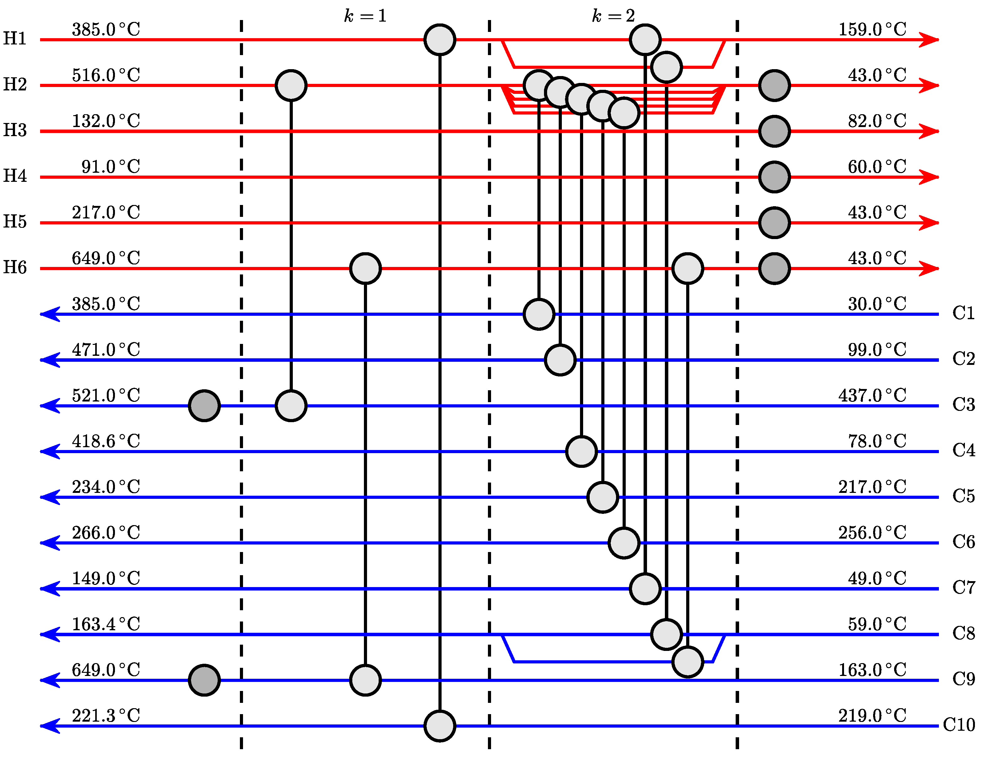
Appendix B. The outlet temperature of the first utility (flue gas) is increased from 800.0 °C to 1674.4 °C. The outlet temperature of the cold utility is lowered from 82.0 °C to 39.6 °C. Therefore, the LMTD at the HEX will be increased, resulting in smaller and more cost-efficient HEX areas. According to
Figure 7, 16.55% and 11.00%, respectively, of the utility heat exchanger cost can be saved.
4. Conclusions
We present an adapted superstructure formulation to consider streams with variable temperatures and flow capacities in the HEN design problem. We use piecewise-linear models with logarithmic coding to leverage the potential of state-of-the-art MILP solvers and to keep the problem traceable. The method is applied to represent utilities as streams. An essential novelty is that utility temperatures and flow capacities do not have to be defined a priori. Instead, only a technically viable range is defined. Further, compared to standard approaches, the utilities can exchange heat at multiple stages with stream splits and do not necessarily have to be placed at the stream ends. By coupling the design optimization of the HEN and the utilities, comprehensive results can be obtained. By increasing the degree of freedom, the holistic process simulation provides the ability to find more efficient HENs and thus reduces costs and resources.
The method presented in this paper was applied to three representative case studies with 4, 9, and 16 streams, respectively. To verify the developed framework, a base case without utility streams was calculated and compared with results from the literature. Our results show only a minor deviation below 1.20% for all case studies, which indicates that our adapted superstructure formulation provides correct results within the expected error range resulting from the piecewise linear approximations and the MIP gap of the solver. To evaluate the potential of unchained HENS, we defined ranges for temperatures and flow capacities for the utilities and compared the results with respect to the base case. For CS1, a cost reduction of 0.29% can be achieved by implementing only the cold utility as a stream. For CS2 and CS3, both the hot and cold utilities were implemented as streams. Cost reductions of 1.30% and 5.37% were achieved, respectively. The results show that in a HEN with utility parameters defined in a specific range, the outlet temperature of cold utilities tends to the lower temperature limit. In contrast, the outlet temperature of hot utilities tends to the upper temperature limit. The resulting small temperature differences between inlet and outlet temperatures at the utilities result in a large LMTD at the heat exchangers. Therefore, the HEX areas can be reduced for the same amount of heat to be transferred, leading to lower TAC. In cases where, for example, the cost structure of the utilities does not depend linearly on the heat to be transferred or the mass flow is limited, a general prediction of the expected temperature is no longer feasible. With our method, these phenomena can be considered, and the coupled optimization of HEN and utilities will lead to cost-optimal results.
Our results of the three representative case studies demonstrate the relevance and versatility of our method. Using multi-stage utilities with stream splits, which do not necessarily have to be located at the stream ends, offers previously untapped potential for efficient utility placement. Loosening strictly defined stream parameters towards the definition of technically permissible ranges additionally generates new possibilities for coupled optimization of utilities and HEN. Moreover, the presented method serves as a foundation to couple the operational characteristics of stream parameter influencing systems into the HENS framework. This will create new opportunities to reduce costs and help to achieve urgently needed emission reduction through holistic process optimization.
Author Contributions
Conceptualization, D.H., F.B. and R.H.; methodology, D.H. and F.B.; formal analysis, D.H. and F.B.; writing—original draft preparation, D.H.; writing—review and editing, D.H., F.B. and R.H.; visualization, D.H.; supervision, F.B. and R.H.; funding acquisition, R.H. All authors have read and agreed to the published version of the manuscript.
Funding
This research was funded by the Austrian Research Promotion Agency (FFG) under grant number 884340 and TU Wien Bibliothek through its Open Access Funding Programme.
Data Availability Statement
No new data were created or analyzed in this study. Data sharing is not applicable to this article.
Acknowledgments
The authors acknowledge TU Wien Bibliothek for financial support through its Open Access Funding Programme.
Conflicts of Interest
The authors declare no conflict of interest.
Nomenclature
| Acronyms |
| CS | case study | |
| CUS | cold utility stream | |
| GA | genetic algorithm | |
| HEN | heat exchanger network | |
| HENS | heat exchanger network synthesis | |
| HEX | heat exchanger | |
| HUS | hot utility stream | |
| MILP | mixed-integer linear programming | |
| PtL | Power-to-Liquid | |
| RMSE | root-mean-square error | |
| SSE | sum of squares error | |
| TAC | total annual cos | |
| US | utility stream | |
| Superscripts |
| in | inlet | |
| out | outlet | |
| v | variable utility paramters | |
| Subscripts |
| cu | cold utility | |
| hu | hot utility | |
| s | stream | |
| i | hot stream | |
| j | cold stream | |
| k | temperature stage | |
| Parameters |
| cost exponent | |
| minimum approach temperature °C | |
| upper bound for temperature difference | °C |
| upper bound for heat exchange | kW |
| lower bound for heat exchange | kW |
| step-fixed HEX cost coefficient | €/y |
| variable HEX cost coefficient | €/m2βy |
| cost coefficient for cold streams | €/kWy |
| cost coefficient for cold utilities | €/kWy |
| cost coefficient for hot streams | €/kWy |
| cost coefficient for hot utilities | €/kWy |
| F | flow capacity | kW/K |
| h | heat transfer coefficient | kW/m2K |
| n | dimension | |
| number of cold streams | |
| number of hot streams | |
| number of stages | |
| U | heat transfer coefficient for matches | kW/m2K |
| Sets |
|
|
|
|
|
|
|
|
|
| Variables |
| temperature difference | K |
| LMTD | logarithmic mean temperature difference | °C |
| TAC | total annual costs | € |
| F | flow capacity | kW/K |
| q | heat flow | kW |
| T | temperature | °C |
| z | binary variable for existance of HEX |
Appendix A. Convergence Behavior
The convergence behavior of the three case studies is based on the log-file of the solver and is shown in
Figure A1,
Figure A2 and
Figure A3. The script to process the unformatted data into processable vectors was coded by ChatGPT [
31].
Figure A1.
Convergence behavior of CS1 for the base and the var UC case.
Figure A1.
Convergence behavior of CS1 for the base and the var UC case.
Figure A2.
Convergence behavior of CS2 for the base and the var UC and UH case.
Figure A2.
Convergence behavior of CS2 for the base and the var UC and UH case.
Figure A3.
Convergence behavior of CS3 for the base and the var UC and UH case.
Figure A3.
Convergence behavior of CS3 for the base and the var UC and UH case.
Appendix B. Stream Plots
Figure A4,
Figure A5,
Figure A6,
Figure A7,
Figure A8 and
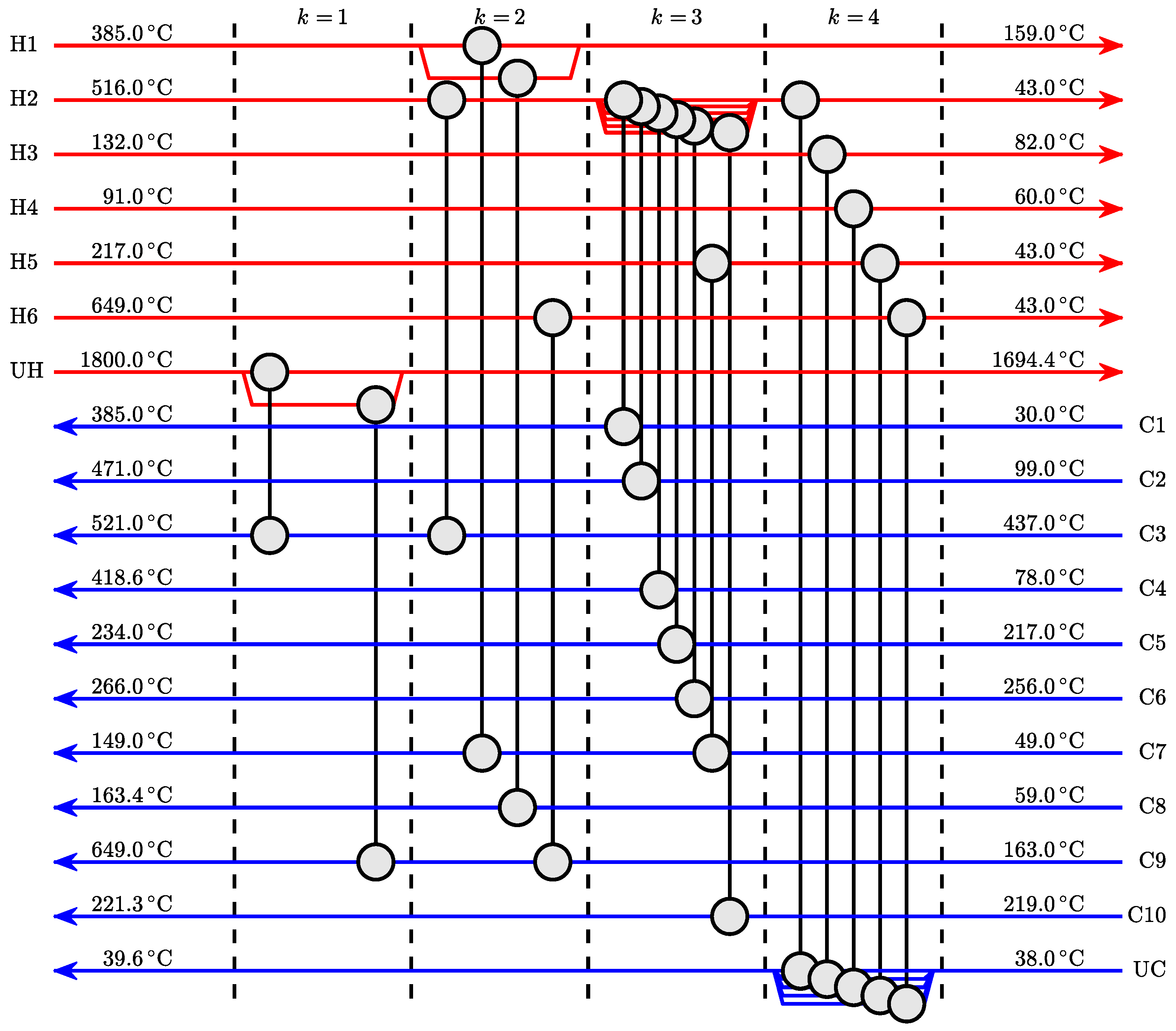
Figure A9 show the optimized stream plots of the three case studies from
Section 3. Hot streams are shown in red, and cold streams are shown in blue. The light gray circles inside the stages
k represent heat exchangers. The dark gray circles without connecting lines are hot and cold utilities, respectively.
Figure A4.
Optimized HEN configuration of CS1: base case with TAC of .
Figure A4.
Optimized HEN configuration of CS1: base case with TAC of .
Figure A5.
Optimized HEN configuration of CS1: var UC case with TAC of .
Figure A5.
Optimized HEN configuration of CS1: var UC case with TAC of .
Figure A6.
Optimized HEN configuration of CS2: base case with TAC of .
Figure A6.
Optimized HEN configuration of CS2: base case with TAC of .
Figure A7.
Optimized HEN configuration of CS2: var UC & UH case with TAC of .
Figure A7.
Optimized HEN configuration of CS2: var UC & UH case with TAC of .
Figure A8.
Optimized HEN configuration of CS3: base case with . Note that in this case only the flue gas is used as a hot utility.
Figure A8.
Optimized HEN configuration of CS3: base case with . Note that in this case only the flue gas is used as a hot utility.
Figure A9.
Optimized HEN configuration of CS3: var UC and UH case with TAC of . Note that in this case only the flue gas is used as a hot utility.
Figure A9.
Optimized HEN configuration of CS3: var UC and UH case with TAC of . Note that in this case only the flue gas is used as a hot utility.
References
- Broeck, H.T. Economic Selection of Exchanger Sizes. Ind. Eng. Chem. 1944, 36, 64–67. [Google Scholar] [CrossRef]
- Masso, A.H.; Rudd, D.F. The synthesis of system designs. II. Heuristic structuring. AIChE J. 1969, 15, 10–17. [Google Scholar] [CrossRef]
- Ciric, A.R.; Floudas, C.A. Heat exchanger network synthesis without decomposition. Comput. Chem. Eng. 1991, 15, 385–396. [Google Scholar] [CrossRef]
- Yuan, X.; Pibouleau, L.; Domenech, S. Experiments in process synthesis via mixed-integer programming. Chem. Eng. Process. Process Intensif. 1989, 25, 99–116. [Google Scholar] [CrossRef]
- Yee, T.F.; Grossmann, I.E. Simultaneous optimization models for heat integration—II. Heat exchanger network synthesis. Comput. Chem. Eng. 1990, 14, 1165–1184. [Google Scholar] [CrossRef]
- Furman, K.C.; Sahinidis, N.V. A Critical Review and Annotated Bibliography for Heat Exchanger Network Synthesis in the 20th Century. Ind. Eng. Chem. Res. 2002, 41, 2335–2370. [Google Scholar] [CrossRef]
- Escobar, M.; Trierweiler, J.O. Optimal heat exchanger network synthesis: A case study comparison. Appl. Therm. Eng. 2013, 51, 801–826. [Google Scholar] [CrossRef]
- Gu, S.; Liu, L.; Zhang, L.; Bai, Y.; Wang, S.; Du, J. Heat exchanger network synthesis integrated with flexibility and controllability. Chin. J. Chem. Eng. 2019, 27, 1474–1484. [Google Scholar] [CrossRef]
- Zirngast, K.; Kravanja, Z.; Novak Pintarič, Z. An improved algorithm for synthesis of heat exchanger network with a large number of uncertain parameters. Energy 2021, 233, 121199. [Google Scholar] [CrossRef]
- Furman, K.C.; Sahinidis, N.V. Computational complexity of heat exchanger network synthesis. Comput. Chem. Eng. 2001, 25, 1371–1390. [Google Scholar] [CrossRef]
- Martelli, E.; Elsido, C.; Mian, A.; Marechal, F. MINLP model and two-stage algorithm for the simultaneous synthesis of heat exchanger networks, utility systems and heat recovery cycles. Comput. Chem. Eng. 2017, 106, 663–689. [Google Scholar] [CrossRef]
- Beck, A.; Hofmann, R. A Novel Approach for Linearization of a MINLP Stage-Wise Superstructure Formulation. Comput. Chem. Eng. 2018, 112, 17–26. [Google Scholar] [CrossRef]
- Vielma, J.P.; Nemhauser, G.L. Modeling disjunctive constraints with a logarithmic number of binary variables and constraints. Math. Program. 2011, 128, 49–72. [Google Scholar] [CrossRef]
- Camm, J.D.; Raturi, A.S.; Tsubakitani, S. Cutting Big M Down to Size. Interfaces 1990, 20, 61–66. [Google Scholar] [CrossRef]
- Löfberg, J. YALMIP: A toolbox for modeling and optimization in MATLAB. In Proceedings of the 2004 IEEE International Conference on Robotics and Automation (IEEE Cat. No.04CH37508), Taipei, Taiwan, 2–4 September 2004; pp. 284–289. [Google Scholar] [CrossRef]
- The MathWorks Inc. MATLAB, Version 9.13.0 (R2022b). 2022. Available online: https://de.mathworks.com/ (accessed on 8 December 2022).
- Ahmad, S. Heat Exchanger Networks: Cost Trade-Offs in Energy and Capital. Ph.D. Thesis, UMIST, Manchester, UK, 1985. [Google Scholar]
- Nielsen, J.S.; Weel Hansen, M.; bay Joergensen, S. Heat exchanger network modelling framework for optimal design and retrofitting. Comput. Chem. Eng. 1996, 20, S249–S254. [Google Scholar] [CrossRef]
- Khorasany, R.M.; Fesanghary, M. A novel approach for synthesis of cost-optimal heat exchanger networks. Comput. Chem. Eng. 2009, 33, 1363–1370. [Google Scholar] [CrossRef]
- Linnhoff, B.; Ahmad, S. Cost optimum heat exchanger networks—1. Minimum energy and capital using simple models for capital cost. Comput. Chem. Eng. 1990, 14, 729–750. [Google Scholar] [CrossRef]
- Fieg, G.; Luo, X.; Jeżowski, J. A monogenetic algorithm for optimal design of large-scale heat exchanger networks. Chem. Eng. Process. Process Intensif. 2009, 48, 1506–1516. [Google Scholar] [CrossRef]
- Lewin, D.R. A generalized method for HEN synthesis using stochastic optimization — II. Comput. Chem. Eng. 1998, 22, 1387–1405. [Google Scholar] [CrossRef]
- Zhu, X.; O’Neil, B.; Roach, J.; Wood, R. A method for automated heat exchanger network synthesis using block decomposition and non-linear optimization. Chem. Eng. Res. Des. 1995, 73, 919–930. [Google Scholar]
- Pavão, L.V.; Costa, C.B.; Ravagnani, M.A. A new stage-wise superstructure for heat exchanger network synthesis considering substages, sub-splits and cross flows. Appl. Therm. Eng. 2018, 143, 719–735. [Google Scholar] [CrossRef]
- Feyli, B.; Soltani, H.; Hajimohammadi, R.; Fallahi-Samberan, M.; Eyvazzadeh, A. A reliable approach for heat exchanger networks synthesis with stream splitting by coupling genetic algorithm with modified quasi-linear programming method. Chem. Eng. Sci. 2022, 248, 117140. [Google Scholar] [CrossRef]
- Nair, S.K.; Karimi, I.A. Unified Heat Exchanger Network Synthesis via a Stageless Superstructure. Ind. Eng. Chem. Res. 2019, 58, 5984–6001. [Google Scholar] [CrossRef]
- Kayange, H.A.; Cui, G.; Xu, Y.; Li, J.; Xiao, Y. Non-structural model for heat exchanger network synthesis allowing for stream splitting. Energy 2020, 201, 117461. [Google Scholar] [CrossRef]
- Aguitoni, M.C.; Pavão, L.V.; Siqueira, P.H.; Jiménez, L.; Ravagnani, M.A.d.S.S. Heat exchanger network synthesis using genetic algorithm and differential evolution. Comput. Chem. Eng. 2018, 117, 82–96. [Google Scholar] [CrossRef]
- Pavão, L.V.; Costa, C.B.B.; Ravagnani, M.A.S.S. An Enhanced Stage-wise Superstructure for Heat Exchanger Networks Synthesis with New Options for Heaters and Coolers Placement. Ind. Eng. Chem. Res. 2018, 57, 2560–2573. [Google Scholar] [CrossRef]
- Liu, Z.; Yang, L.; Yang, S.; Qian, Y. An extended stage-wise superstructure for heat exchanger network synthesis with intermediate placement of multiple utilities. Energy 2022, 248, 123372. [Google Scholar] [CrossRef]
- OpenAI. Assistant. 2022. Available online: https://chat.openai.com/ (accessed on 21 December 2022).
Figure 1.
Piecewise-linear approximation of the reduced stream HEX area as a function of the heat flow q and LMTD with five hyperplanes. Hot stream: , , , . Cold stream: , , , . . .
Figure 1.
Piecewise-linear approximation of the reduced stream HEX area as a function of the heat flow q and LMTD with five hyperplanes. Hot stream: , , , . Cold stream: , , , . . .
Figure 2.
Piecewise-linear approximation of the reduced utility HEX area as a function of the heat flow q with four lines. Hot stream: , , , . Cold utility: , , . . .
Figure 2.
Piecewise-linear approximation of the reduced utility HEX area as a function of the heat flow q with four lines. Hot stream: , , , . Cold utility: , , . . .
Figure 3.
Piecewise-linear approximation of the stream-wise energy balance as a function of the flow capacity F and the temperature difference with 32 simplices. Hot stream: , , . .
Figure 3.
Piecewise-linear approximation of the stream-wise energy balance as a function of the flow capacity F and the temperature difference with 32 simplices. Hot stream: , , . .
Figure 4.
Piecewise-linear approximation of the LMTD as a function of the two temperature differences and . LMTD in the range from 10 K to 200 K. .
Figure 4.
Piecewise-linear approximation of the LMTD as a function of the two temperature differences and . LMTD in the range from 10 K to 200 K. .
Figure 5.
Breakdown of the cost structure for CS1. Relative cost savings in relation to the cost components of the base case.
Figure 5.
Breakdown of the cost structure for CS1. Relative cost savings in relation to the cost components of the base case.
Figure 6.
Breakdown of the cost structure for CS2. Relative cost savings in relation to the cost components of the base case.
Figure 6.
Breakdown of the cost structure for CS2. Relative cost savings in relation to the cost components of the base case.
Figure 7.
Breakdown of the cost structure for CS3. Relative cost savings in relation to the cost components of the base case.
Figure 7.
Breakdown of the cost structure for CS3. Relative cost savings in relation to the cost components of the base case.
Table 1.
Stream data for case study 1: Ahmad [
17].
Table 1.
Stream data for case study 1: Ahmad [
17].
| Stream | / °C | / °C | F / kW/K | h / kW/m2/K |
|---|
| H1 | 260 | 160 | 3.0 | 0.4 |
| H2 | 250 | 130 | 1.5 | 0.4 |
| C1 | 120 | 235 | 2.0 | 0.4 |
| C2 | 180 | 240 | 4.0 | 0.4 |
| UH | 280 | 279 | - | 0.4 |
| UC | 30 | 80 | - | 0.4 |
| UCv | 30 | [31, 80] | (0, 20] | 0.4 |
Table 2.
Problem size, computation time and relative gap for CS1.
Table 2.
Problem size, computation time and relative gap for CS1.
| Case | Variables / - | Binaries / - | Time / s | Rel. Gap / % |
|---|
| base | 321 | 120 | 2.30 | 0.0000 |
| var UC | 3610 | 376 | 22.79 | 0.0009 |
Table 3.
Results for CS1: Comparison of costs and heat loads at the utilities and streams.
Table 3.
Results for CS1: Comparison of costs and heat loads at the utilities and streams.
| Reference | | Heat Load / kW |
|---|
| TAC / 104 $/y | CU | HU | Stream |
|---|
| Ahmad [17] | 1.2870 | 60.00 | 50.00 | 420.00 |
| Nielsen et al. [18] | 1.2306 | 45.00 | 36.00 | 434.00 |
| Khorasany & Fesanghary [19] | 1.1895 | 28.10 | 18.10 | 451.91 |
| this work—base | 1.1792 | 25.52 | 15.52 | 454.48 |
| this work—var UC | 1.1767 | 25.59 | 15.59 | 454.41 |
Table 4.
Stream data for case study 2: Linnhoff & Ahmad [
20].
Table 4.
Stream data for case study 2: Linnhoff & Ahmad [
20].
| Stream | / °C | / °C | F / kW/K | h / kW/m2/K |
|---|
| H1 | 327 | 40 | 100 | 0.50 |
| H2 | 220 | 160 | 160 | 0.40 |
| H3 | 220 | 60 | 60 | 0.14 |
| H4 | 160 | 45 | 400 | 0.30 |
| C1 | 100 | 300 | 100 | 0.35 |
| C2 | 35 | 164 | 70 | 0.70 |
| C3 | 85 | 138 | 350 | 0.50 |
| C4 | 60 | 170 | 60 | 0.14 |
| C5 | 140 | 300 | 200 | 0.60 |
| UH | 330 | 250 | - | 0.50 |
| UHv | 330 | [329, 250] | (0, 25,000] | 0.50 |
| UC | 15 | 30 | - | 0.50 |
| UCv | 15 | [16, 30] | (0, 35,000] | 0.50 |
Table 5.
Problem size, computation time, and relative gap for CS2.
Table 5.
Problem size, computation time, and relative gap for CS2.
| Case | Variables / - | Binaries / - | Time / s | Rel. Gap / % |
|---|
| base | 1009 | 387 | 133.95 | 0.0096 |
| var UC & UH | 3014 | 1201 | 590.12 | 0.0000 |
Table 6.
Results for CS2: Comparison of costs and heat loads at the utilities and streams.
Table 6.
Results for CS2: Comparison of costs and heat loads at the utilities and streams.
| Reference | | Heat Load / MW |
|---|
| TAC / 106 $/y | CU | HU | Stream |
|---|
| Linnhoff & Ahmad [20] a | 2.9300 | 32.76 | 25.04 | 61.14 |
| Linnhoff & Ahmad [20] b | 2.8900 | 33.03 | 25.31 | 60.87 |
| Zhu et al. [23] | 2.9700 | 33.94 | 26.22 | /* |
| Lewin [22] | 2.9360 | 32.81 | 25.09 | 61.09 |
| Fieg et al. [21] | 2.9223 | 31.34 | 23.62 | 62.57 |
| this work—base | 2.9114 | 31.42 | 23.70 | 62.48 |
| this work—var UC & UH | 2.8526 | 31.43 | 23.71 | 62.47 |
Table 7.
Stream data for case study 3: Khorasany and Fesanghary [
19].
Table 7.
Stream data for case study 3: Khorasany and Fesanghary [
19].
| Stream | / °C | / °C | F / kW/K | h / kW/m2/K |
|---|
| H1 | 385.0 | 159.0 | 131.51 | 1.238 |
| H2 | 516.0 | 43.0 | 1198.96 | 0.546 |
| H3 | 132.0 | 82.0 | 378.96 | 0.771 |
| H4 | 91.0 | 60.0 | 589.55 | 0.859 |
| H5 | 217.0 | 43.0 | 186.22 | 1.000 |
| H6 | 649.0 | 43.0 | 116.00 | 1.000 |
| C1 | 30.0 | 385.0 | 119.10 | 1.850 |
| C2 | 99.0 | 471.0 | 191.05 | 1.129 |
| C3 | 437.0 | 521.0 | 377.91 | 0.815 |
| C4 | 78.0 | 418.6 | 160.43 | 1.000 |
| C5 | 217.0 | 234.0 | 1297.70 | 0.443 |
| C6 | 256.0 | 266.0 | 2753.00 | 2.085 |
| C7 | 49.0 | 149.0 | 197.39 | 1.000 |
| C8 | 59.0 | 163.4 | 123.56 | 1.063 |
| C9 | 163.0 | 649.0 | 95.98 | 1.810 |
| C10 | 219.0 | 221.3 | 1997.50 | 1.377 |
| UH1 | 1800.0 | 800.0 | - | 1.200 |
| UH | 1800.0 | [800.0, 1700.0] | (0, 150.00] | 1.200 |
| UH2 | 509.0 | 509.0 | - | 1.000 |
| UC | 38.0 | 82.0 | - | 1.000 |
| UCv | 38.0 | [39.0, 82.0] | [10,000, 500,000] | 1.000 |
Table 8.
Problem size, computation time, and relative gap for CS3.
Table 8.
Problem size, computation time, and relative gap for CS3.
| Case | Variables / - | Binaries / - | Time / s | Rel. Gap / % |
|---|
| base | 2893 | 1128 | 637.07 | 0.0094 |
| var UC & UH | 7302 | 2914 | 11,335.64 | 0.0100 |
Table 9.
Results for CS3: Comparison of costs and heat loads at the utilities and streams.
Table 9.
Results for CS3: Comparison of costs and heat loads at the utilities and streams.
| Reference | | Heat Load / MW |
|---|
| TAC / 106 $/y | CU | HU | Stream |
|---|
| existing plant [19] | 8.8564 | 524.72 | 122.16 | /* |
| Khorasany & Fesanghary [19] | 7.4357 | 469.62 | 66.07 | 267.09 |
| Feyli et al. [25] | 7.1285 | 437.77 | 34.21 | 298.96 |
| Aguitoni et al. [28] | 7.1028 | 437.44 | 33.87 | 299.29 |
| Pavão et al. [29] | 6.8013 | 414.03 | 10.47 | 322.69 |
| Pavão et al. [24] | 6.7126 | 413.07 | 9.50 | 323.65 |
| Nair & Karimi [26] | 6.6956 | 412.25 | 8.69 | 324.47 |
| Liu et al. [30] | 6.6647 | 413.11 | 9.55 | 323.61 |
| this work—base | 6.7451 | 414.72 | 11.13 | 322.04 |
| this work—var UC & UH | 6.3297 | 416.57 | 12.98 | 320.18 |
| Disclaimer/Publisher’s Note: The statements, opinions and data contained in all publications are solely those of the individual author(s) and contributor(s) and not of MDPI and/or the editor(s). MDPI and/or the editor(s) disclaim responsibility for any injury to people or property resulting from any ideas, methods, instructions or products referred to in the content. |
© 2023 by the authors. Licensee MDPI, Basel, Switzerland. This article is an open access article distributed under the terms and conditions of the Creative Commons Attribution (CC BY) license (https://creativecommons.org/licenses/by/4.0/).


