Determination of 12 Combustion Products, Flame Temperature and Laminar Burning Velocity of Saudi LPG Using Numerical Methods Coded in a MATLAB Application

Abstract

The characterization of a specific fuel has always been an important point for developing and designing new components or systems with the maximum efficient possible. Studying the laminar burning velocity can lay a necessary prerequisite for the accurate poststudy of the turbulent range and to understand how the combustion process takes place. The study of the combustion products from a specific reaction is a requisite for any system in order to understand the elements that are taken in the process and if it is possible to improve it. In this study, a new open code methodology was developed for the determination of combustion products, flame temperature and laminar burning velocity using numerical methods (Newton–Raphson, Taylor series and Gaussian elimination) in an application codified in MATLAB. The MATLAB application was applied for the study of Saudi LPG setting parameters such as initial temperature, pressure and equivalence ratio that are meaningful because they have a great effect on the results. In addition, simulation in Ansys Chemkin using San Diego and RedSD mechanisms was carried out. The results from the MATLAB application were compared with other experimental research and Ansys Chemkin simulation. These are presented in different plots and it is shown that: (1) For the laminar burning velocity results, the numerical method agrees with the experimental results for ratios (0.6–1.2) by other authors and the simulation in Ansys Chemkin. (2) For the highest studied equivalence ratios (1.3–1.7) the laminar burning velocity results between all the resources have more difference. (3) The combustion products calculated by the MATLAB application agree with those simulated in Ansys Chemkin except N and NO. (4) The MATLAB application gives a maximum value of 40.35 cm/s, that is greater than 35 ± 0.91, the one determined by Bader A. Alfarraj. (5) The flame temperature calculated by the MATLAB application overestimates that simulated in Ansys Chemkin but has the same behavior for all the calculated ratios. (6) The MATLAB application has also been developed for the study and analysis of other fuels.

1. Introduction

The analysis and study of the most used fuels in the world allow us to continue extracting and improving all the information collected to date. Liquefied petroleum gas is one of the fuels with the most applications in all fields, for example: combustion engines, ovens, burners, industries, etc. To better understand this fuel, it is necessary to determine and study the properties that characterize it, which a posteriori allow optimizing the devices that use it in order to obtain a balance between performance and efficiency. Among the main characteristics and properties are the flame temperature, the laminar burning velocity and the products of combustion. The laminar burning velocity is one of the most fundamental characteristics of the combustion of a certain mixture, likewise, it contains fundamental information on reactivity, diffusivity and exotherm, therefore, it is used to characterize the flames and precise knowledge is important for the equipment design, turbulent combustion model and validation of chemical kinetic mechanisms [1]. The burning velocity for any type of fuel mixture is affected by different factors, the main ones are pressure, temperature, equivalence ratio (Φ) and the properties of the fuel components [2].

To obtain the flame speed theoretically and experimentally, studies and methods were developed many years ago. On one hand, the oldest ones date back to 1949, when Powling and Edgerton developed a flat flame burner which allowed a close approximation to the ideal of a one-dimensional flat flame, but it was limited to low flame velocities (0.15–0.2 m/s) [1]. On the other hand, more recent studies such as that of Samahat Samim in 2016, which investigated the determination of the laminar flame speeds of gas to liquid (GTL) fuel with conventional diesel (50–50 by volume) in a cylindrical pump, were able to measure the flame speed at initial temperatures and atmospheric pressure equivalence ratios, by analyzing the pressures just after combustion, which were detected by a pressure transducer installed in the pump and, as a conclusion, the blended fuel was determined to have the lowest flame velocity at the highest temperature (89.7 cm/s at 250 °C) [1,3].

Regarding the investigations on the laminar flame speed of LPG, in 2004 Kihyung Lee and Jeaduk Ryu conducted a study of the flame propagation and combustion characteristics of this fuel using an optical technique for measurement of flame velocity in a constant volume combustion chamber (CVCC) and a heavy duty liquefied petroleum liquid injection (LPLi) port [4]. Later, in 2007, A.S. Huzayyin, H.A. Moneib, M.S. Shehatta and A.M.A. Attia determined the variations of the laminar flame velocity and the explosion rates of LPG–air mixtures in a wide range of equivalence ratios (Φ = 0.7–2.2), initial temperatures (Ti = 295–400 K) and pressures (Pi = 50–400 kPa) where they used a cylindrical combustion pump [5]. Three years later, Ajay Tripathi, H. Chandra and M. Agrawal studied the flame speed of LPG–air and LPG–air–diluent (CO₂) mixtures at different values of equivalence ratio and diluent concentration using two experimental methods: Bunsen burner and cylindrical tube [6]. In the same year, Domnina Razus, Venera Brinzea, Maria Mitu and Dumitru Oancea determined the laminar flame speeds of LPG–air and LPG–air–exhaust mixtures from pressure vs. time graphs obtained from a spherical container with central ignition, making use of a correlation based on the cubic law of the pressure increase during the initial phase of the explosion at different fuel/oxygen ratios and in different environmental conditions [7]. Later, in 2016, Ahmed Yasiry and Haroun Shahad carried out an experimental study of the laminar flame speed of Iraqi LPG using a constant volume chamber with central ignition at different initial pressures (0.1–0.3 MPa) and an initial temperature of 308 K. Likewise, a range of equivalence ratios from 0.8 to 1.3 were used [8]. Recently, in the year 2022, Bader Alfarraj, Ahmed Al-Harbi, Saud A. Binjuwair and Abdullah Alkhedhair carried out the characterization of the Saudi LPG using a Bunsen burner and a modified Bunsen burner, which allowed them to work in a range of equivalence ratios of 0.68 to 1.3 [9].

In this study, mathematical methodology coded in a MATLAB application was developed with the main idea of giving a contribution to the scientific community of an open code program in an easy tool that can be used by any researcher or student involved in this kind of study. It was found that most of the studies carried out by researchers on numerical methods are quite complex and do not include an interactive way to see, compare and analyze the results, which is one of the most valuable characteristics that the MATLAB application has. In addition, the application has the option to be improved by anyone by adding other functions or assumptions that can grow its range of application and accuracy. The MATLAB application was used for the determination of the main combustion characteristics of Saudi LPG (flame temperature, combustion products and laminar burning velocity) studied in the investigation by Bader Alfarraj, Ahmed Al-Harbi, Saud A. Binjuwair and Abdullah Alkhedhair [9]. The limitations of the application are that it can be only applied to hydrocarbon fuels, including oxygen and/or nitrogen or not; the flame temperature cannot exceed 3725 °C and cannot be lower than 327 °C; and the equivalence ratio cannot be too high so it does not allow the formation of free carbon. Moreover, as part of the research, simulation was carried out in Ansys Chemkin using the San Diego [10] and RedSD [11] mechanisms to obtain these properties, with the aim of extending the research carried out by these authors by using a simple numerical method.

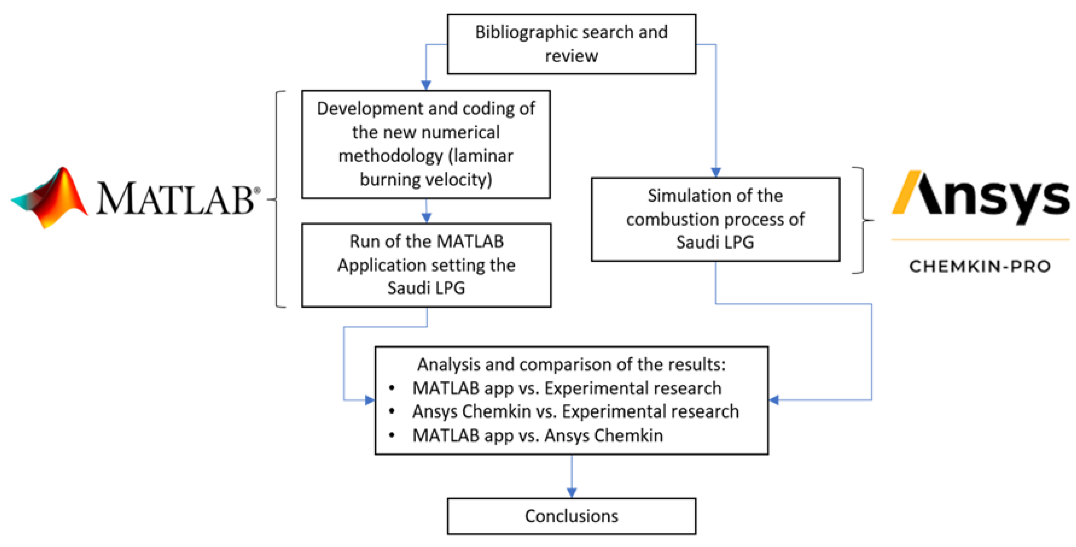
2. Materials and Methods

2.1. Materials and Procedure

A computer with an AMD Ryzen 7 5700 G with Radeon Graphics 3.80 GHz processor with 32 GB RAM and Windows 11 Enterprise operating system was used for coding in MATLAB version R2021b and simulation in Ansys Chemkin R2 2022. For the Ansys Chemkin simulation the San Diego mechanism and RedSD mechanism were used. The general procedure can be seen in Figure 1.

2.2. Numerical Methodology for the Determination of Combustion Products and Flame Temperature

For the determination of the combustion products and their molar fractions, the numerical methodology developed in FORTRAN by Olikara and Borman in 1975 [12] was coded in MATLAB, using numerical methods such as Taylor series, Newton–Raphson and Gaussian elimination. To start with the methodology, Equation (1) is proposed as the equation corresponding to the combustion reaction and starting point for the formulation of the following equations, with the fuel being C_n + H_m + O_l + N_k, the equivalence ratio Φ, X₁→X₁₂ as the mole fractions of the products and x₁₃ as the number of moles from fuel that give 1 mol of products.

X₁₃[C_n + H_m + O_l + N_k + ((n + 0.25 ∗ m − 0.5 ∗ l)/Φ) (O₂ + 3.7274N₂ + 0.0444Ar)] →
X₁H + X₂O + X₃N + X₄H₂ + X₅OH + X₆CO + X₇NO + X₈O₂ + X₉H₂O + X₁₀CO₂ + X₁₁N₂ + X₁₂Ar

(1)

The reactant part can also be written as

X₁₃[nC + mH + rO₂ + r′N₂ + r″Ar],

(2)

with the equivalences for r, r′, r″ as

r = l/2 + r_o,

(3)

r′ = k/2 + 3.7274 r_o,

(4)

r″ = 0.0444 r_o,

(5)

r_o = (n + 0.25 ∗ m − 0.5 ∗ l)/Φ.

(6)

Setting the balance of the elements of the reaction and considering that all the products must add up to 1, five equations for each element are obtained: carbon, hydrogen, oxygen, nitrogen and argon, respectively, and an additional one for the sum of fractions of the products equivalent to unity.

X₆ + X₁₀ = n ∗ X₁₃,

(7)

X₁ + 2X₄ + X₅ + 2X₉ = m ∗ X₁₃,

(8)

X₂ + X₅ + X₆ + X₇ + 2X₈ + X₉ + 2X₁₀ = 2r ∗ X₁₃,

(9)

X₃ + X₇ + 2X₁₁ = 2r’ ∗ X_13,

(10)

X₁₂ = r’’ ∗ X₁₃,

(11)

X₁ + X₂ + X₃ + X₄ + X₅ + X₆ + X₇ + X₈ + X₉ + X₁₀ + X₁₁ + X₁₂ = 1.

(12)

In order to solve the equations system, 7 additional equations are required so 7 chemical reactions are considered in this situation, and they were selected for the benefit of the products that were set in Equation (1).

½ H₂ ↔ H,

(13)

½ O₂ ↔ O,

(14)

½ N₂ ↔ N,

(15)

½ H₂ + ½ O₂ ↔ OH,

(16)

½ O₂ + ½ N₂ ↔ NO,

(17)

H₂ + ½ O₂ ↔ H₂O,

(18)

CO + ½ O₂ ↔ CO₂,

(19)

and each chemical reaction has a partial pressure equilibrium constant, which are presented in the same order as their chemical reaction:

K₁ = X₁ ∗ p^1/2/X₄^1/2,

(20)

K₂ = X₂ ∗ p^1/2/X₈^1/2,

(21)

K₃ = X₃ ∗ p^1/2/X₁₁^1/2,

(22)

K₅ = X₅/(X₄^1/2 ∗ X₈^1/2),

(23)

K₇ = X₇/(X₈^1/2 ∗ X₁₁^1/2),

(24)

K₉ = X₉/(X₄ ∗ X₈^1/2 ∗ p^1/2),

(25)

K₁₀ = X₁₀/(X₆ ∗ X₈^1/2 ∗ p^1/2).

(26)

It is important to mention that each of the equilibrium constants at partial pressure (Equations (20)–(26)) was adjusted in the range of 327 °C to 3725 °C using the tables and properties from JANAF Thermodynamical Tables 1985 [13], so the MATLAB application has this limitation. The general equation that adjusts all the constants and their respective coefficients can be found in the paper of Olikara and Borman [12]. Using the equations of the constants for each reaction and of Equations (20)–(26), the respective constants (C_n) can be set for each combustion product, which will remain for every equation with X₄, X₆, X₈ and X₁₁ pressure as the only variables. In this way,

X₁ = C₁ ∗ X₄^1/2, where C₁ = K₁/p^1/2,

(27)

X₂ = C₂ ∗ X₈^1/2, where C₂ = K₂/p^1/2,

(28)

X₃ = C₂ ∗ X₈^1/2, where C₃ = K₃/p^1/2,

(29)

X₅ = C₅ ∗ X₄ ∗ X₈^1/2, where C₅ = K₅,

(30)

X₇ = C₇ ∗ X₈^1/2 ∗ X₁₁^1/2, where C₇ = K₇,

(31)

X₉ = C₉ ∗ X₄ ∗ X₈^1/2, where C₉ = K₉ ∗ p^1/2,

(32)

X₁₀ = C₁₀ ∗ X₆ ∗ X₈^1/2, where C₁₀ = K₁₀ ∗ p^1/2,

(33)

are the equations to set the equation system. In order to set the system, it is necessary to define

X₁₂ = r″X₁₃ = r″(X₆ + X₁₀)/n,

(34)

using (7) and (11). With (34) it is possible to eliminate X₁₂ and X₁₃ from (7)–(12) and form

X₁ + 2X₄ + X₅ + 2X₉ – m ∗ (X₆ + X₁₀)/n = 0,

(35)

X₂ + X₅ + X₆ + X₇ + X₉ + 2X₁₀ − 2r ∗ (X₆ + X₁₀)/n = 0,

(36)

X₃ + X₇ + 2X₁₁ − 2r′/n (X₆ + X₁₀) = 0,

(37)

X₁ + X₂ + X₃ + X₄ + X₅ + X₆ + X₇ + X₈ + X₉ + X₁₀ + X₁₁ + r″(X₆ + X₁₀)/n − 1 = 0.

(38)

Using (27)–(33) in (35)–(38) it is possible to obtain the system equation with just 4 variables (X₄, X₆, X₈ and X₁₁). The equation system is a non-linear system with 4 variables whose general representation is

f_j (X₄, X₆, X₈, X₁₁) = 0, j = 1, 2, 3, 4.

(39)

In order to solve the equation system, a Taylor series is applied to linearize the system. For applying the Taylor series, it is a requisite to know a vector,

[X₄⁽¹⁾, X₆⁽¹⁾, X₈⁽¹⁾, X₁₁⁽¹⁾],

(40)

that is near to the solution vector

[X₄*, X₆*, X₈*, X₁₁*],

(41)

For each of the equations on the left side of the system (Equation (39)), they can be expanded around the solution vector to obtain

∆X_i = X_i* − X_i⁽¹⁾, i = 4, 6, 8, 11.

(42)

Deriving each expression and ignoring partial derivatives of which the order is higher than 1, it is possible to obtain the linear equation

f_j + (∂f_j/∂X₄) ∆X₄ + (∂f_j/∂X₆) ∆X₆ + (∂f_j/∂X₈) ∆X₈ + (∂f_j/∂X₁₁) ∆X₁₁ ≅ 0, j = 1, 2, 3, 4,

(43)

in which the derivatives are evaluated in the known vector. Using the Gauss elimination method, it is possible to solve the new linear system and obtain the values of ∆X₄, ∆X₆, ∆X₈, ∆X₁₁ that will be useful to bring the known vector closer to the solution vector by applying

X_i⁽²⁾ = X_i⁽¹⁾ + ∆X_i, i = 4, 6, 8, 11.

(44)

in which X_i⁽²⁾ is the improved vector which is entered into (43) in order to obtain another improvement. This process is repeated the necessary times until the values of ∆X₄, ∆X₆, ∆X₈, ∆X₁₁ are less than or equal to 0.0001, which is the maximum error margin considered for each molar fraction.

Moreover, for the calculation of the adiabatic flame temperature, the equivalence between the reactants and the products is applied as

h(T, p_o, F_o) − h_r(T_o, p_o, F_o) = 0.

(45)

It is necessary to obtain an improved temperature, so the Newton–Raphson is defined as

T_{n + 1} = T_n − (h(T_n, p_o, F_o) − h_r)/(∂h/∂T)_n.

(46)

in which T_n is the first assumed temperature (preferably greater than the final temperature), h_r is the reactant enthalpy at initial conditions of temperature (T_o), pressure (p_o) and equivalence ratio (F_o), h(T_n, p_o, F_o) is obtained once the combustion products are calculated at the first assumed temperature (T_n) as

h(T_n, p_o, F_o) = ∑X_ih_i/M,

(47)

this last equation can be derived with respect to temperature and it will give

∂h/∂T = 1/M [∑(X_i dh_i/dT + h_i dX_i/dT) − ∂M/∂T h(T_n, p_o, F_o)],

(48)

in which dh_i/dT is the specific heat at a constant pressure of each element, so

dh_i/dT = Cp_i,

(49)

where dX_i/dT is calculated using (27)–(33) and ∂M/∂T is the molar mass of the mixture with respect to the temperature, that is,

∂M/∂T = ∑ dX_i/dT (M_i).

(50)

Finally, the Newton–Raphson iteration concludes when

(h(T_n, p_o, F_o) − h_r)/(∂h/∂T)_n ≤ 1

(51)

In order to start this procedure, it is necessary to know the vector (40) that is near to the solution vector (41), and the steps to obtain it are mentioned in detail in the paper of Olikara and Borman [11]. Furthermore, all the partial derivatives with respect to temperature, pressure and equivalence ratio of each element can be found in the same source.

2.3. Determination of the Laminar Burning Velocity

For the determination of the laminar burning velocity, the adiabatic flame temperature previously calculated is directly replaced in

S_L = (e^−Ea/RuT)^1/2

(52)

that corresponds to the Mallard and Le Chateller theory. Ea is the activation energy, R_u is the universal gas constant (1.987 cal/mol·K) and T is the flame temperature calculated using the method. The value for Ea for every calculation is taken from the average of two values. The first one is set according to Kenneth Kuo, who said that for most hydrocarbon reactions the energy of activation is around 120 kJ/mol [2]. The second one is from Markatou, who studied methane–air oxidation and determined an activation energy of approximately 130 kJ/mol [14], so the average is 125 kJ/mol or 29,675.7 cal/mol.

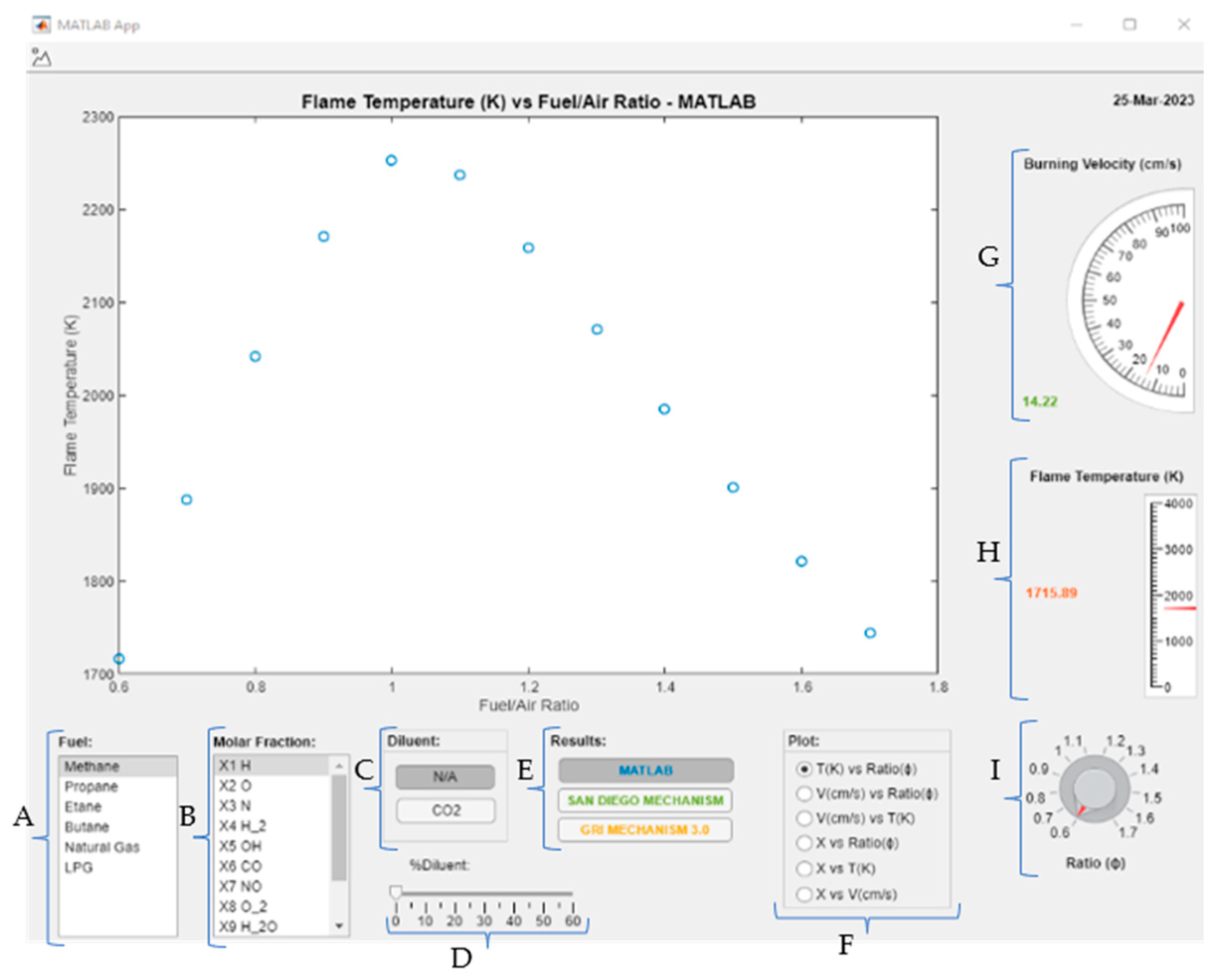
2.4. Development of the MATLAB Application

2.4.1. First Part: New_Code.m

All of the procedure and steps described in Section 2.2 and Section 2.3 were codified in the MATLAB application to be directly used just by setting the fuel and, in some cases, the diluents available (CO₂). The first part of the code corresponds to the archive called New_code.m, which can be found in Code S1, having defined as inputs the equivalence ratio, percentage of diluent if applicable, name of diluent and name of fuel. The indices of each element of the selected fuel (C, H, O, N) are stored in an Excel archive called Reactants_Enthalpy.xlsx and those of the diluents in Reactants_Diluents.xlsx, and they can be found in Archives S1 and S2. In order to improve the application range of the MATLAB application, it is possible to add more fuels and diluents to Archives S1 and S2.

Moreover, the determination of the reactant enthalpy (h_r) is carried out, for which the initial temperature and pressure of work will always be 298 K and 1 atm, respectively. After the first steps are carried out, New_code.m enters into a loop in order to obtain the combustion products by calling the function Fractions_Derivatives.m and, after it, the first assumed temperature is adjusted with the value calculated in (51) or “DELTA” which is the name used in the code.

In case the DELTA is less than or equal to 1, the laminar burning velocity is calculated and the iteration process finished. On the other hand, in case is not is not less than or equal to 1, the loop continues adjusting the combustion products and the adiabatic flame temperature.

2.4.2. Second Part: Fractions_Derivatives.m

This second part corresponds to the archive called Fractions_Derivatives.m, whose code can be found in Code S2, which determines the twelve combustion products by setting a matrix equation system and solving it by using a for loop in order to apply the Gaussian elimination method using row interchange. In other words, it uses Equations (3)–(6) to carry out the simplification of the combustion reaction elements, Equations (7)–(12) for the balance of the elements and Equations (20)–(33) for setting all the molar fractions with respect to X₄, X₆, X₈ and X₁₁ using the 7 chemical reactions as a starting point (Equations (13)–(19)). Additional to this, Equations (35)–(38) are set in order to obtain the equation system (39) in which the Taylor series is applied to linearize the system and the Gaussian elimination method is applied to solve the linearized system.

By the same method, a matrix equation system is set and solve for the derivatives of each molar fraction with respect to temperature, equivalence ratio and pressure using a maximum pivot strategy.

When the molar fractions are adjusted, the product enthalpy, the derivative of the enthalpy with respect to temperature and the combustion products’ molar fractions are given to New_code.m that calculates by using the Newton–Raphson method in the enthalpy equation balance, that is, Equation (45), in order to obtain

(∂h/∂T)_n,

(53)

The process runs until it fulfills the tolerance for the final flame temperature and laminar burning velocity is calculated. For solving both matrix equation systems, constants and some variables are set in order to form the system, such as the partial pressure equilibrium constant for each reaction. Archive S4 (Products.xlsx) includes the thermodynamical properties of the combustion products in order to obtain the correct DELTA.

2.4.3. Third Part: Developing the MATLAB Application in the MATLAB App Designer Interface

In order to create the app archive, the App Designer interface is used. The MATLAB code of the application can be found in Code S3. It is possible to see in Figure 2 some tools and buttons that will help the user to obtain and analyze the information.

Table 1. Tools available in the MATLAB application.

Position in Figure 2	Name of Tool	Description	Type of Selection
A	Fuel list	List of fuels available for calculus in the application	Unique
B	Molar fraction list	List of molar fractions available for plotting results	Unique
C	Diluent button list	List of diluents available to use in the calculus	Unique
D	Percentage bar of diluent	Percentage of diluent by volume to be considered in fuel	Unique
E	Results button list	Results from resources available to be shown in the plot	Multi
F	Plot button list	Type of plot to be shown on the screen	Unique
G	Equivalence ratio knob	Knob that shows the value of laminar burning velocity and flame temperature in their respective gauges	Unique
H	Laminar burning velocity gauge	Laminar burning velocity value at the knob equivalence ratio value selected	NA
I	Flame temperature gauge	Flame temperature value at the knob equivalence ratio value selected	NA

details the information about each tool available in the application.

Figure 3 gives an example of the fuel and results selection; it shows the plot results for the molar fraction of the hydrogen (H₂) vs. equivalence ratio for the LPG with 10% CO₂ obtained just by two resources (MATLAB code and San Diego mechanism). The equivalence ratio knob is also set at the stoichiometric value so the flame temperature and laminar burning velocity values are shown for that ratio value in their respective gauges (H and I).

2.5. Composition of Fuel and Mixtures to Be Tested

The fuel to be analyzed and set in the application as a newly available option is the Saudi LPG, whose composition is 50% propane (C₃H₈) and 50% butane (C₄H₁₀) and is the same used by Bader Alfarraj et al. [9]. The tested mixtures are from 0.6 to 1.7, increasing by 0.1. As was mentioned previously, the initial conditions are 298 K for temperature and 1 atm of pressure.

2.6. Simulation in Ansys Chemkin

The simulation is carried out in Ansys Chemkin 2022 R2 using the San Diego mechanism (57 species) and RedSD mechanism (47 species). The reason for choosing these two mechanisms is the good agreement for simulations using propane and butane. Both follow the idea of having a small number of species and reactions for the scope of combustion, and this gives accurate results. In addition to this, the limitation of 70 species in the Ansys Chemkin 2022 R2 has an influence. Reduced San Diego (RedSD) is a reduced mechanism developed in the Department of Mechanical Engineering, Indian Institute of Technology Madras, Chennai, India from the San Diego mechanism [10] by S.M. Kumaran, D. Shanmugasundaram, K. Narayanaswamy and V. Raghavan in 2021 [11]. This compact mechanism was comprehensively validated against experimental data on flames using 1D and 2D computations. The 1D computations of premixed and non-premixed flames are carried out using Flame Master and Chemkin-Pro, while 2D axisymmetric calculations are performed within Ansys Fluent, taking into account multicomponent diffusion, thermal diffusion and radiation sub-models [11]. In general, the results obtained show that the 45 species mechanism is able to predict the desired combustion characteristics in different types of flames of propane, n-butane and their mixtures satisfactorily [11]. The principal parameters of initial temperature, pressure of work and equivalence ratios are configured with the same values of the calculations in the MATLAB application. Figure 4 presents the flow diagram in the Ansys Chemkin software for the simulation. All the results are in Ansys Chemkin Results (0.6–1.7).xlsx, which can be found in Archive S3.

3. Results and Discussion

The results for the numerical method run by the MATLAB application are presented for the twelve combustion products, flame temperature and laminar burning velocity and compared with the Ansys Chemkin simulation.

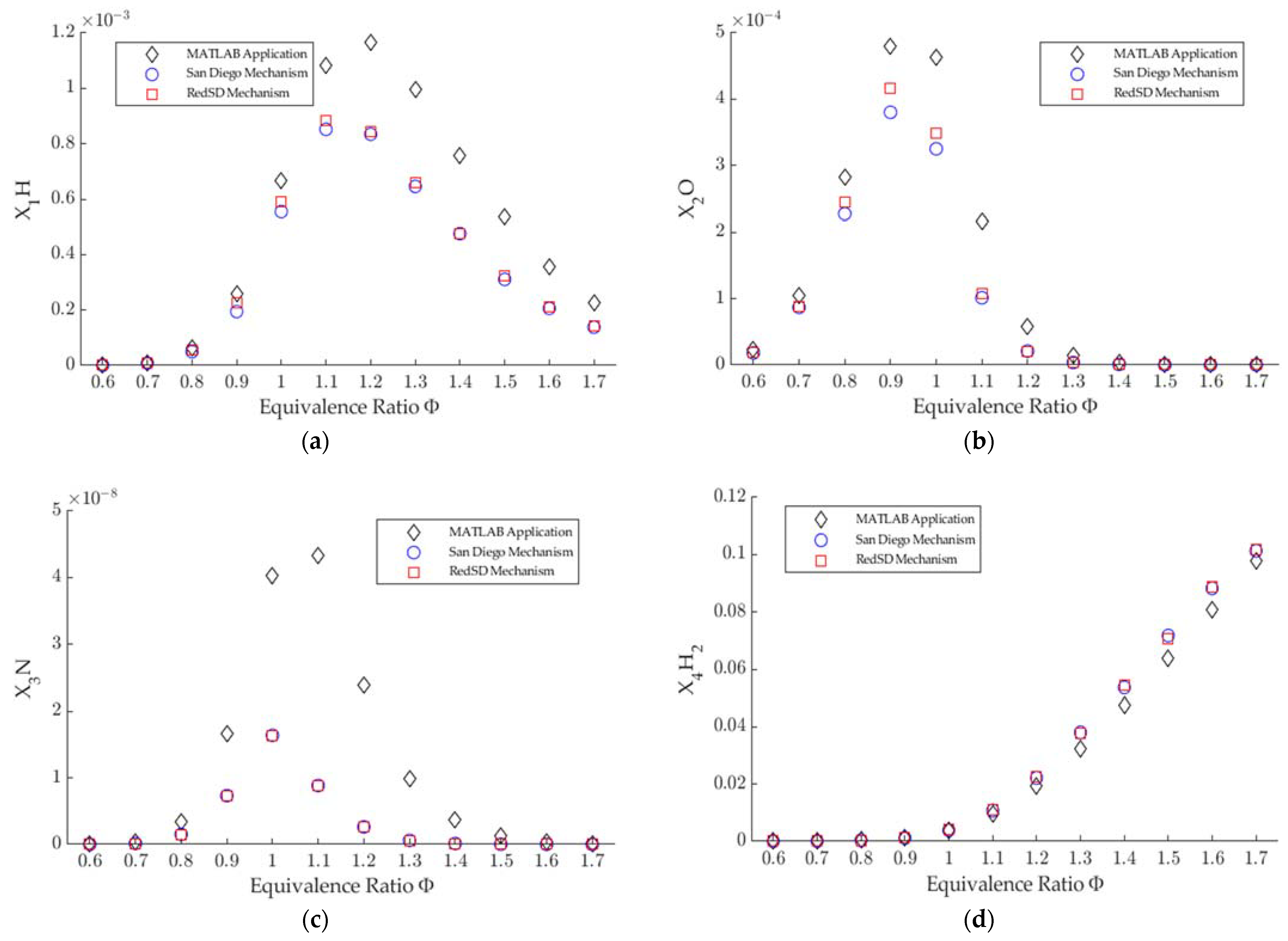
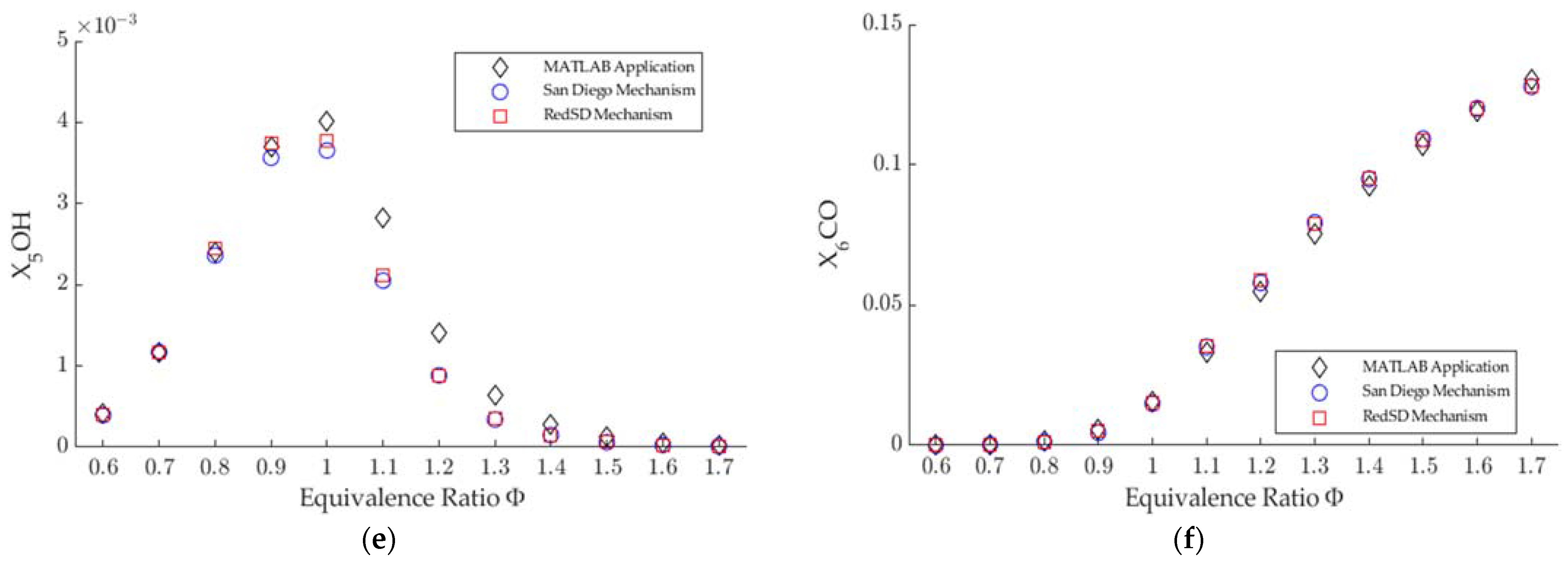
3.1. Combustion Products

The numerical method run by the MATLAB application for the mixtures of Saudi LPG gives the molar fractions of the combustion products values presented in

Table 2. Combustion Products of Saudi LPG (X₁–X₆) calculated by MATLAB application.

Equivalence Ratio (Φ)	X1H	X2O	X3N	X4H2	X5OH	X6CO
0.6	9.2644 × 10−7	2.3773 × 10−5	1.6175 × 10−11	1.2640 × 10−5	0.00041207	3.5819 × 10−5
0.7	1.0249 × 10−5	0.00010408	3.4726 × 10−10	8.5230 × 10−5	0.0011626	0.00028795
0.8	6.5024 × 10−5	0.00028288	3.4003 × 10−9	0.00039475	0.00240522	0.0015017
0.9	0.00025914	0.00048031	1.6695 × 10−8	0.00138214	0.00369457	0.00556398
1	0.00066624	0.00046349	4.0295 × 10−8	0.00393763	0.00401577	0.0154476
1.1	0.00108218	0.00021577	4.3271 × 10−8	0.00962653	0.00281794	0.0331991
1.2	0.00116468	5.8248 × 10−5	2.3838 × 10−8	0.0194133	0.00141014	0.0549746
1.3	0.00099712	1.3753 × 10−5	9.9015 × 10−9	0.0323431	0.00063771	0.075101
1.4	0.00075851	3.2136 × 10−6	3.6705 × 10−9	0.047353	0.00028167	0.0922573
1.5	0.00053636	7.5281 × 10−7	1.2757 × 10−9	0.0636388	0.00012302	0.106798
1.6	0.00035653	1.7192 × 10−7	4.1393 × 10−10	0.0806081	5.2459 × 10−5	0.119274
1.7	0.00022589	3.8207 × 10−8	1.2688 × 10−10	0.097815	2.1858 × 10−5	0.13018

(X₁–X₆) and

Table 3. Combustion Products of Saudi LPG (X₇–X₁₂) calculated by MATLAB application.

Equivalence Ratio (Φ)	X7NO	X8O2	X9H2O	X10CO2	X11N2	X12AR
0.6	0.00232901	0.0786287	0.0935573	0.0729014	0.743231	0.00886708
0.7	0.00353978	0.0575011	0.107843	0.084112	0.73656	0.00879482
0.8	0.00436595	0.0373029	0.121284	0.094098	0.729583	0.00871664
0.9	0.00425856	0.0196666	0.133438	0.100834	0.721799	0.00862329
1	0.00300759	0.0071197	0.143566	0.101098	0.712176	0.0085012
1.1	0.0013496	0.00141652	0.150092	0.0925431	0.699319	0.00833818
1.2	0.00044049	0.00019234	0.151587	0.0790268	0.683587	0.00814537
1.3	0.00013844	2.6966 × 10−5	0.148982	0.0665658	0.667245	0.0079489
1.4	4.4765 × 10−5	4.1781 × 10−6	0.143582	0.056652	0.651305	0.00775848
1.5	1.4838 × 10−5	6.9691 × 10−7	0.136333	0.0489914	0.635987	0.00757583
1.6	4.9101 × 10−6	1.1887 × 10−7	0.127913	0.0430682	0.621321	0.00740107
1.7	1.6125 × 10−6	2.0403 × 10−8	0.118823	0.0384122	0.607287	0.00723388

(X₇–X₁₂).

It is possible to see from Table 2 and Table 3 that the most predominant fractions in lean mixtures are X₈O₂, X₉H₂O, X₁₀CO₂ and X₁₁N₂. This is an expected result and it is the first proof that the MATLAB application method agrees with the general combustion theory statements (lean mixture, excess of oxygen, greater percentage of oxygen in the products). As the equivalence ratio increases, X₈O₂ decreases and X₁₀CO₂ decreases while X₆CO increases, which agrees with rich mixtures, in other words, there is not enough oxygen for the combustion process. Considering Equation (19), it is not possible to transform CO to CO₂. Moreover, the results obtained by carrying out the simulation in Ansys Chemkin using the San Diego mechanism are presented in

Table 4. Combustion Products of Saudi LPG (X₁–X₆) using San Diego mechanism.

Equivalence Ratio (Φ)	X1H	X2O	X3N	X4H2	X5OH	X6CO
0.6	6.6093 × 10−7	1.8192 × 10−5	3.5006 × 10−12	1.0017 × 10−5	0.00039345	2.7661 × 10−5
0.7	8.3166 × 10−6	8.693 × 10−5	1.3135 × 10−10	7.4804 × 10−5	0.00117059	0.00024538
0.8	4.9654 × 10−5	0.00022725	1.4973 × 10−9	0.00033309	0.00236175	0.00123292
0.9	0.00019441	0.00038015	7.3197 × 10−9	0.00114976	0.00356367	0.00454945
1	0.00055523	0.00032513	1.6402 × 10−8	0.00388401	0.00365408	0.0149326
1.1	0.00085203	0.00010131	8.8505 × 10−9	0.0107692	0.00205185	0.0351553
1.2	0.00083450	2.1024 × 10−5	2.6195 × 10−9	0.0221748	0.00088483	0.058047
1.3	0.00064603	3.7060 × 10−6	5.9878 × 10−10	0.0380662	0.00034043	0.0792958
1.4	0.00047560	8.6550 × 10−7	1.3136 × 10−10	0.0536471	0.00014997	0.0948882
1.5	0.00031061	1.7192 × 10−7	1.7254 × 10−11	0.0717481	6.0068 × 10−5	0.109207
1.6	0.00020575	4.1360 × 10−8	1.9497 × 10−12	0.0882793	2.6349 × 10−5	0.120062
1.7	0.00013802	1.1794 × 10−8	2.8318 × 10−13	0.101292	1.2937 × 10−5	0.12784

(X₁–X₆) and

Table 5. Combustion Products of Saudi LPG (X₇–X₁₂) using San Diego mechanism.

Equivalence Ratio (Φ)	X7NO	X8O2	X9H2O	X10CO2	X11N2	X12AR
0.6	1.2659 × 10−6	0.0778787	0.0957267	0.0734329	0.0743441	0.00906312
0.7	1.0758 × 10−5	0.0564053	0.111239	0.0849199	0.73685	0.00898358
0.8	7.4972 × 10−5	0.0364389	0.124853	0.0951511	0.730366	0.00890481
0.9	0.00028322	0.0190562	0.136546	0.102239	0.723214	0.00881881
1	0.00036887	0.00517981	0.147765	0.102416	0.712228	0.00868567
1.1	8.0115 × 10−5	0.00060559	0.15336	0.0911168	0.697399	0.00850336
1.2	1.8270 × 10−5	6.1474 × 10−5	0.153406	0.076219	0.680035	0.0082915
1.3	3.9921 × 10−6	6.2188 × 10−6	0.149864	0.0628266	0.660878	0.00805869
1.4	7.1151 × 10−7	9.9641 × 10−7	0.143506	0.0540122	0.645431	0.00786988
1.5	8.0017 × 10−8	1.4057 × 10−7	0.135334	0.0466537	0.628933	0.00766906
1.6	2.5797 × 10−8	2.5968 × 10−8	0.127036	0.0415919	0.614249	0.00749027
1.7	1.1576 × 10−8	6.0938 × 10−9	0.119289	0.0384194	0.602665	0.00734881

(X₇–X₁₂). It is important to mention that there were more combustion products in the results given by Ansys Chemkin such as propane and butane that did not manage to react and this can be seen principally at higher equivalence ratios (1.2–1.7). The results using RedSD mechanism are presented in

Table 6. Combustion Products of Saudi LPG (X₁–X₆) using RedSD mechanism.

Equivalence Ratio (Φ)	X1H	X2O	X3N	X4H2	X5OH	X6CO
0.6	6.9492 × 10−7	1.8833 × 10−5	3.5006 × 10−12	1.0326 × 10−5	0.00039894	2.8759 × 10−5
0.7	8.4643 × 10−6	8.8159 × 10−5	1.3135 × 10−10	7.5337 × 10−5	0.00117376	0.00024771
0.8	5.5236 × 10−5	0.00024429	1.4973 × 10−9	0.00035698	0.00244458	0.00132638
0.9	0.00022744	0.00041572	7.3197 × 10−9	0.0012917	0.00374339	0.00510691
1	0.00059085	0.00034823	1.6402 × 10−8	0.00399172	0.00377842	0.015321
1.1	0.00088504	0.00010743	8.8505 × 10−9	0.0108747	0.00211538	0.0354616
1.2	0.00084480	2.0644 × 10−5	2.6195 × 10−9	0.0226464	0.00087630	0.0588178
1.3	0.00066097	3.9565 × 10−6	5.9878 × 10−10	0.0377389	0.00035226	0.0789434
1.4	0.00047605	8.4477 × 10−7	1.3136 × 10−10	0.0542954	0.00014795	0.0952242
1.5	0.00032336	1.9393 × 10−7	1.7254 × 10−11	0.0706793	6.4263 × 10−5	0.108435
1.6	0.00021240	4.3565 × 10−8	1.9497 × 10−12	0.0887154	2.7351 × 10−5	0.120091
1.7	0.00014340	1.2649 × 10−8	2.8318 × 10−13	0.101579	1.3416 × 10−5	0.127924

(X₁–X6) and

Table 7. Combustion Products of Saudi LPG (X₇–X₁₂) using RedSD mechanism.

Equivalence Ratio (Φ)	X7NO	X8O2	X9H2O	X10CO2	X11N2	X12AR
0.6	1.2659 × 10−6	0.0778787	0.0957267	0.0734329	0.0743441	0.00906312
0.7	1.0758 × 10−5	0.0564053	0.111239	0.0849199	0.73685	0.00898358
0.8	7.4972 × 10−5	0.0364389	0.124853	0.0951511	0.730366	0.00890481
0.9	0.00028322	0.0190562	0.136546	0.102239	0.723214	0.00881881
1	0.00036887	0.00517981	0.147765	0.102416	0.712228	0.00868567
1.1	8.0115 × 10−5	0.00060559	0.15336	0.0911168	0.697399	0.00850336
1.2	1.8270 × 10−5	6.1474 × 10−5	0.153406	0.076219	0.680035	0.0082915
1.3	3.9921 × 10−6	6.2188 × 10−6	0.149864	0.0628266	0.660878	0.00805869
1.4	7.1151 × 10−7	9.9641 × 10−7	0.143506	0.0540122	0.645431	0.00786988
1.5	8.0017 × 10−8	1.4057 × 10−7	0.135334	0.0466537	0.628933	0.00766906
1.6	2.5797 × 10−8	2.5968 × 10−8	0.127036	0.0415919	0.614249	0.00749027
1.7	1.1576 × 10−8	6.0938 × 10−9	0.119289	0.0384194	0.602665	0.00734881

(X₇–X12).

Figure 5a–f show the behavior differences between the results from the MATLAB application and the simulation in Ansys Chemkin from X₁ to X₆, while Figure 6a–f show the results from X₇ to X₁₂. From Figure 5d,f it can be affirmed for all cases that only hydrogen (X₄H₂) and carbon monoxide (X₆CO) had an increase as the equivalence ratio increased. This is mainly a consequence of the increase in the amount of fuel in the mixture and the lack of oxygen in it to finish transforming these variables into hydrogen hydroxide (X₉H₂O) and carbon dioxide (X₁₀CO₂), respectively, which is shown by the fall in the fractions corresponding to those products at a higher equivalence ratio. On the other hand, nitrogen (X₁₁N₂) and argon (X₁₂AR) presented a decrease for all cases as the equivalence ratio increased because of the opposite effect that this change has on the elements that compound the oxidization, in this case, air.

Likewise, another product that presents the same trend, but in a more predominant way, is oxygen (X₈O₂), whose value, in cases of a higher ratio, tends to practically zero. Similarly, in the case of hydroxide (X₅OH), there is a tendency to zero for its values at the highest equivalence ratio and this is due to the lack of molecular oxygen to complete the whole reaction (16). Regarding the similarity and difference in the results for all cases, in general, there exists a correlation between those determined by the MATLAB application and simulation in Ansys Chemkin using the San Diego mechanism and RedSD mechanism, specifically for X₄H₂, X₅OH, X₆CO, X₈O₂, X₉H₂O, X₁₀CO₂, X₁₁N₂, X₁₂AR, whose values presented the same evolutionary curve between all the sources as the value of the equivalence ratio varied.

Furthermore, taking as a reference the results of the simulation in Ansys Chemkin using the San Diego mechanism, because it is the most complete mechanism (greater number of species and reactions) of the two tested, the smallest differences for the cases X₉, X₁₀, X₁₁, X₁₂ were found, being 3.05%, 5.95%, 1.15%, 2.22%, respectively.

3.2. Flame Temperature

Saudi LPG/air mixtures tested using the MATLAB application and simulation in Ansys Chemkin using San Diego and RedSD mechanisms gave the results presented in

Table 8. Results for flame temperature.

Equivalence Ratio (Φ)	MATLAB Application T (K)	San Diego Mechanism T (K)	RedSD Mechanism T (K)
0.6	1763.1	1723.7	1721.8
0.7	1945.7	1914.3	1911.5
0.8	2108.1	2076.8	2075.6
0.9	2238.6	2202.8	2206.0
1	2318.5	2283.9	2283.3
1.1	2326.2	2267.3	2268.9
1.2	2272.7	2198.0	2196.9
1.3	2197.8	2109.6	2111.1
1.4	2118.8	2033.4	2031.4
1.5	2040.1	1956.1	1961.1
1.6	1963.1	1889.2	1889.0
1.7	1888.0	1831.0	1831.7

for flame temperature.

Figure 7 shows the results for the flame temperature and the differences between the three methods. It was found that the flame temperatures of the mixtures tested using the MATLAB application were higher than those simulated in Ansys Chemkin using San Diego and RedSD mechanisms. In addition to this, it can be observed that the flame temperature was the maximum in the stoichiometric mixture for the Ansys Chemkin test cases, however, in the case of the MATLAB application, the maximum value was found for an equivalence ratio of 1.1.

The gap between the results from the MATLAB application and simulation in Ansys Chemkin is correct according to the MATLAB application calculation of the adiabatic temperature, considering a balance between enthalpies of reactants and products, while Ansys Chemkin simulation included the loss of heat from the mixture to the to the burner walls by convection, the subsequent loss by convection of the walls to the outside and the heat loss from the flame to the outside, therefore, the flame temperature determined by the two mechanisms must be lower. Moreover, it is possible to validate the formation of N and NO that was presented in Figure 5c and Figure 6a, respectively, which occurs at higher temperatures, and therefore a higher fraction was obtained for the results using the MATLAB application in comparison with the simulation in Ansys Chemkin. In addition, the absolute difference and its percentage between the results for the three cases are presented in

Table 9. Flame temperature differences between the MATLAB application and simulations in Ansys Chemkin.

Equivalence Ratio (Φ)	MATLAB Application—San Diego Mechanism		MATLAB Application—RedSD Mechanism
	∆T (K)	%	∆T (K)	%
0.6	39.4	2.2	41.2	2.4
0.7	31.3	1.6	34.1	1.7
0.8	31.2	1.5	32.4	1.5
0.9	35.8	1.6	32.6	1.4
1	34.5	1.5	35.1	1.5
1.1	58.5	2.6	57.3	2.5
1.2	74.7	3.4	75.8	3.4
1.3	88.1	4.1	86.7	4.1
1.4	85.4	4.2	87.4	4.3
1.5	84.0	4.3	79.0	4.0
1.6	73.8	3.9	74.0	3.9
1.7	57.0	3.1	56.3	3.0

. It can be affirmed that, on average, there was a difference of 57.89 K and 2.86% for the results between the MATLAB application and those obtained through simulation in Ansys Chemkin using the San Diego mechanism. In addition to this, an average difference of 57.7 K and 2.85% was obtained between the MATLAB application results and simulation in Ansys Chemkin using the RedSD mechanism.

For the San Diego mechanism, the minimum difference was found at an equivalence ration of 0.8 with a difference value of 31.21 K and a percentage of 1.50%, while the maximum difference was found at an equivalence ratio of 1.3 with a difference value of 88.19 K and a percentage of 4.18%. For the RedSD mechanism, the minimum difference was found at an equivalence ratio of 0.8 with a difference value of 32.41 K and a percentage of 1.56%, while the maximum difference was found at an equivalence ratio of 1.4 with a difference value of 87.42 K and a percentage of 4.30%. With these two statements, one for each mechanism, it can be affirmed for flame temperature calculations that the MATLAB application has a percentage of confidence greater than or equal to 95%.

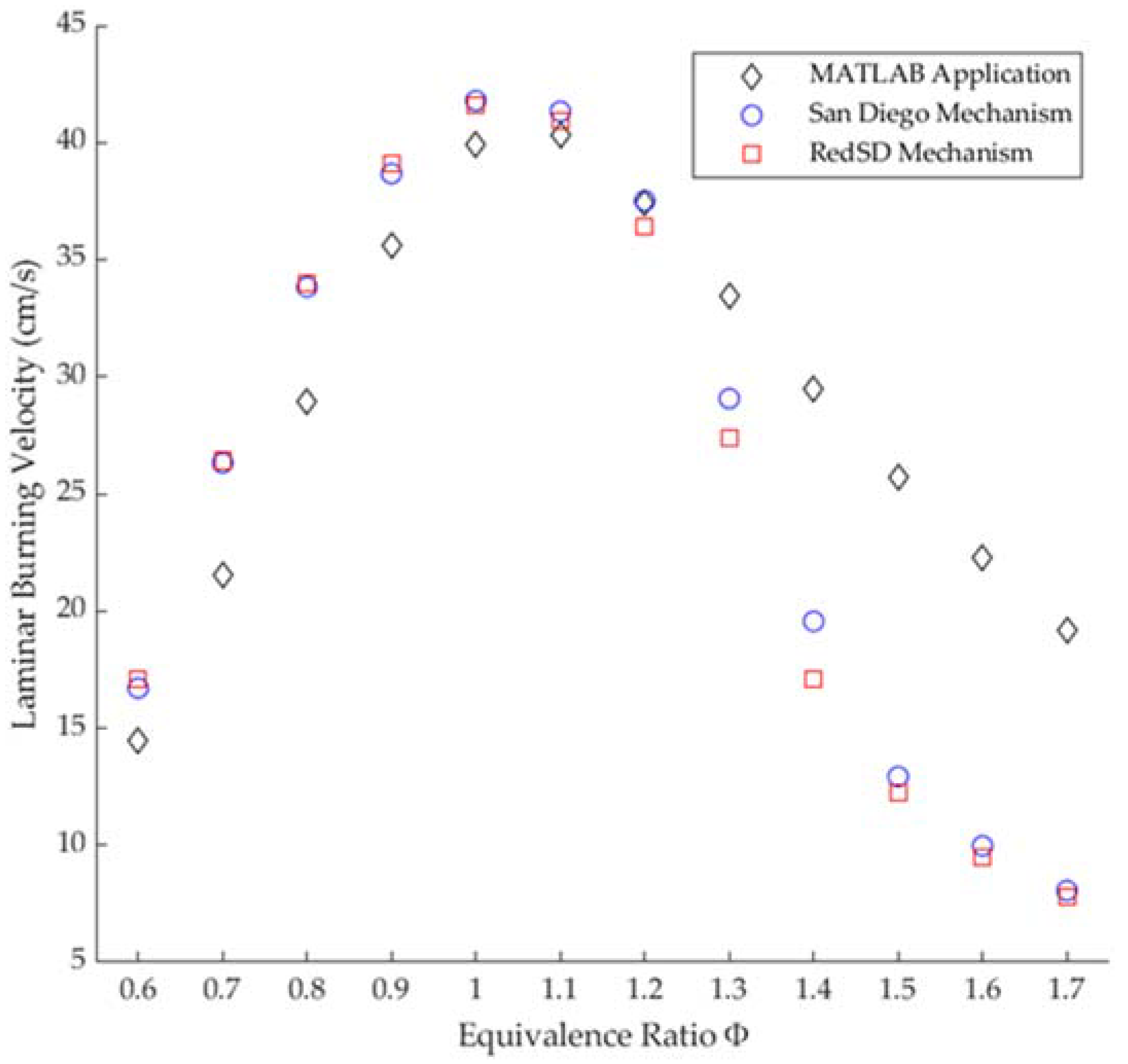
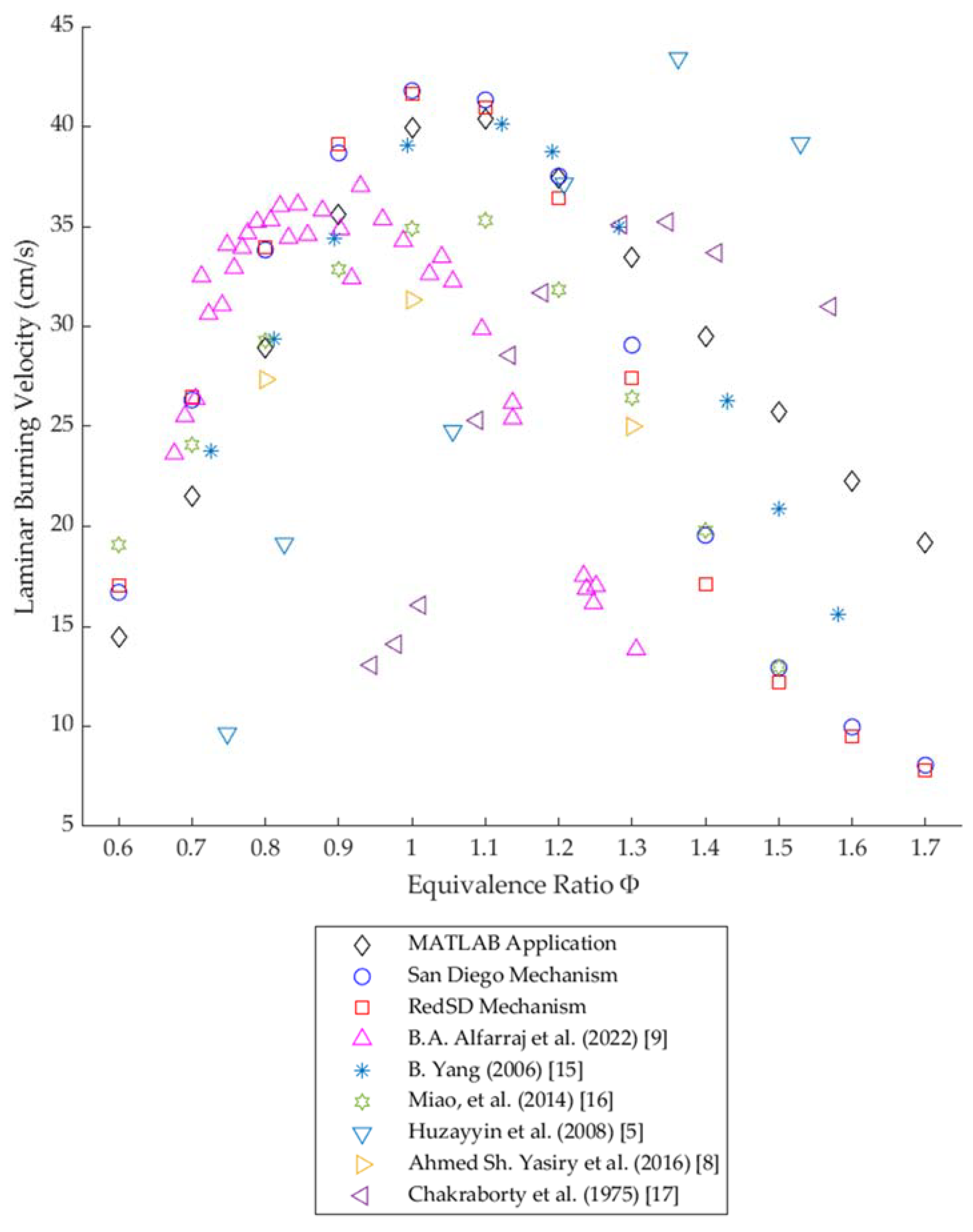
3.3. Laminar Burning Velocity

Saudi LPG/air mixtures tested using the MATLAB application and simulation in Ansys Chemkin using San Diego and RedSD mechanisms gave the results presented in

Table 10. Results for laminar burning velocity.

Equivalence Ratio (Φ)	MATLAB Application SL (cm/s)	San Diego Mechanism SL (cm/s)	RedSD Mechanism SL (cm/s)
0.6	14.4	16.7	17.0
0.7	21.5	26.3	26.4
0.8	28.9	33.8	33.9
0.9	35.5	38.6	39.1
1	39.9	41.7	41.6
1.1	40.3	41.3	40.9
1.2	37.4	37.5	36.4
1.3	33.4	29.0	27.3
1.4	29.4	19.5	17.1
1.5	25.7	12.9	12.2
1.6	22.2	9.9	9.5
1.7	19.1	8.0	7.7

for laminar burning velocity.

From Figure 8, it can be seen that with the increase in equivalence ratio until the stoichiometric condition, the adiabatic temperature and laminar burning velocity increase and, afterward, the adiabatic temperature and laminar burning velocity start decreasing according to the results obtained by using the MATLAB application. On the other hand, with the increase in equivalence ratio until 1.1, the adiabatic temperature and laminar burning velocity increase and, afterward, the adiabatic temperature and laminar burning velocity start decreasing according to the results obtained by simulation in Ansys Chemkin using San Diego and RedSD mechanisms. Furthermore, according to the results for the laminar burning velocity and the differences between the three methods, it was found that the laminar burning velocities of the mixtures tested using the MATLAB application were lower than those simulated in Ansys Chemkin for equivalence ratios less than or equal to 1.2, but they were higher than those simulated in Ansys Chemkin for higher equivalence ratios. In addition to this, the laminar flame speed is the maximum at an equivalence ratio of 1 for both simulations and at 1.1 for the MATLAB application.

It is worth noting that the laminar flame speed is not only influenced by flame temperature, it also has a stretch relationship with parameters such as ambient temperature and pressure, kinetic mechanisms and reactions that occur during combustion. None of these additional factors is considered in the Mallard and Le Chateller method and are considered in the simulation in Ansys Chemkin, so the differences between the results are mainly caused by these factors. The activation energy in the equation of the Mallard and Le Chateller method gives an additional percentage of error for the results obtained by the MATLAB application, which happens because, for each reaction, there is a specific energy of activation, and this is defined in the kinetic data of the mechanisms used in Ansys Chemkin and not in the MATLAB application. In addition to this, for higher equivalence ratios (higher than 1.2) there will exist other combustion products (unburned fuel—C₃H₈ or C₄H₁₀, NO_X, among others, that appeared in the Ansys Chemkin simulations) that cause the difference to increase, as can be seen in Figure 8. This does not happen for lower ratios. A better approximation for the calculation and another improvement for this application is to define an activation energy as a function of the equivalence ratio and temperature, taking as a reference the reactions considered in the MATLAB application and adding the ones involved directly with the tested fuel.

Moreover, the differences between the results and their percentages for the three cases are presented in

Table 11. This is a table. Tables should be placed in the main text near to the first time they are cited.

Equivalence Ratio (Φ)	MATLAB Application—San Diego Mechanism		MATLAB Application—RedSD Mechanism
	∆SL (cm/s)	%	∆SL (cm/s)	%
0.6	−2.2	−13.3	−2.5	−15.1
0.7	−4.7	−18.1	−4.9	−18.6
0.8	−4.8	−14.4	−5.0	−14.8
0.9	−3.0	−7.9	−3.5	−9.0
1	−1.8	−4.4	−1.7	−4.0
1.1	−0.9	−2.3	−0.5	−1.4
1.2	−0.1	−0.2	0.9	2.6
1.3	4.3	15.0	6.0	22.1
1.4	9.9	50.7	12.3	72.3
1.5	12.8	99.0	13.5	110.6
1.6	12.3	123.5	12.7	134.6
1.7	11.1	137.7	11.3	145.9

. It is possible to affirm that the results of the MATLAB application are similar to what is simulated in Ansys Chemkin between ratios of 0.6 to 1.2, according to which percentage differences are not higher than 20. The average found for the absolute differences between the values of the MATLAB application and simulation in Ansys Chemkin using the San Diego mechanism is 5.70 cm/s with a percentage average difference of 40.59%, while the simulation in Ansys Chemkin using the RedSD mechanism gave an average difference of 6.28 cm/s and a percentage of average difference of 45.96%.

Furthermore, the minimum and maximum absolute difference values found were 0.1 cm/s (0.26%) at an equivalence ratio of 1.2 and 12.8 cm/s (99.06%) at an equivalence ratio of 1.5 for the comparative case between the MATLAB application and simulation in Ansys using the San Diego mechanism, while, for the comparative case between the MATLAB application and the simulation in Ansys Chemkin using the RedSD mechanism, the minimum value was 0.59 cm/s (1.45%) at an equivalence ratio of 1.1 and the maximum value was 13.52 cm/s (110.69%) at an equivalence ratio of 1.5.

Figure 9 shows the comparison between the results for laminar burning velocity results obtained in this work and the ones obtained in the investigations of B. A. Alfarraj et al. [9], B. Yang [15], Miao et al. [16], Huzayyin et al. [5], Ahmed Sh. Yasiry et al. [8] and Chakraborty et al. [17]. The composition and details of the LPG used in each work are presented in

Table 12. LPG laminar burning velocity study specifications.

Work	Type of Study	Pressure (atm)	Initial Temperature (K)	LPG Composition
				Propane C3H8	Butane C4H10	Ethane C2H6	Pentane C5H12
MATLAB Application—Current Work	Numerical methodology in MATLAB	1	298.15	50%	50%	0%	0%
San Diego Mechanism—Current Work	Numerical Simulation in Ansys Chemkin	1	298.15	50%	50%	0%	0%
RedSD Mechanism—Current Work	Numerical Simulation in Ansys Chemkin	1	298.15	50%	50%	0%	0%
B.A. Alfarraj et al. [9]	Experimental—Modified Bunsen Burner Method	1	298.15	50%	50%	0%	0%
B. Yang [15]	Experimental—Constant Volume Bomb Method	1	298.15	50%	50%	0%	0%
Huzayyin et al. [5]	Experimental—Constant Volume Chamber Method	1	294 ± 3	26.41%	73.54%	0.04%	0%
Ahmed Sh. Yasiry et al. [8]	Experimental—Constant Volume Chamber Method	1	308	36.3%	62.3%	0.9%	0.5%
Miao et al. [16]	Experimental—Constant Volume Chamber Method	1	298.15	30%	70%	0%	0%
Chakraborty et al. [17]	Experimental—Flat Flame Burner Method	1	298	30.1%	67.7%	1.4%	0%

.

From Figure 9, it can be seen that results obtained using the MATLAB application and simulation in Ansys Chemkin present the same plot shape as the results obtained by Miao et al. [16], B. Yang [15] and B.A. Alfarraj et al. (2022) [9] for ratios under the stoichiometric and fuel-rich conditions. It has to be considered that Miao et al. [16] used a different LPG composition (30% propane and 70% butane) while B. Yang [15] and B.A. Alfarraj et al. (2022) [9] used the same composition in the mixture. On the other hand, for stoichiometric and fuel-rich conditions, the results of the MATLAB application present the same plot shape as the results of B. Yang (2006) [15].

It is important to consider the type of study and instruments the authors of these experimental studies used. Of those who have been mentioned in the previous paragraph, Miao et al. [16] and B. Yang [15] used the constant volume chamber method, which is the most controlled condition for carrying out the experiment (regarding temperature and pressure values) from all of those mentioned in Table 12. Meanwhile, B.A. Alfarraj et al. (2022) [9] used the modified Bunsen burner method in order to have more controlled conditions during the experiments.

Using the results from the previous paragraph, it is possible to affirm that the MATLAB application has similar results to those found using the constant volume chamber method for the whole range of equivalence ratios.

4. Conclusions

In this work, a numerical method was coded in a MATLAB application for the study of Saudi LPG combustion characteristics (products of combustion, the adiabatic flame temperature and the laminar flame velocity), and the results were compared with the results of a simulation in Ansys Chemkin using the San Diego and RedSD mechanisms and other investigations. The following conclusions were reached:

• For the laminar burning velocity results, the numerical method agrees with the experimental results for ratios (0.6–1.2) used by other authors and the simulation carried out in Ansys Chemkin, while, for the highest studied equivalence ratios (1.3–1.7) the laminar burning velocity results show a greater difference between all the resources.
• The numerical method used in the MATLAB application agrees with the simulation in Ansys Chemkin for the Saudi LPG combustion products, except for N and NO, for the whole range of equivalence ratios.
• The Saudi LPG maximum laminar burning velocity determined by the modified Bunsen burner method [9] was 35 ± 0.91 while that determined by the MATLAB application was 40.3 cm/s, having a difference of 5.35 ± 0.91 and an overestimate of 15.2% in favor of the MATLAB application.
• The Saudi LPG maximum laminar burning velocity determined by the MATLAB application was 40.3 cm/s, corresponding to a ratio of 1.1, with an underestimate of 2.3% with respect to the simulated values in Ansys Chemkin using the San Diego mechanism and an underestimate of 1.4% using the RedSD mechanism.
• The maximum adiabatic flame temperature of the Saudi LPG determined using the MATLAB application was 2326.2 K, corresponding to a ratio of 1.1, with an overestimate of 2.6% and 2.5% with respect to the simulated values in Ansys Chemkin using the San Diego and RedSD mechanisms, respectively.
• The MATLAB application, compared with previous experimental studies, presents the same behavioral results as those obtained by Miao et al. [16], B. Yang [15] and B.A. Alfarraj et al. (2022) [9] for lean mixture conditions. Meanwhile, for stoichiometric and fuel-rich conditions, it presents the same plot shape as that of B. Yang (2006) [15].
• The new code in the MATLAB application determined the experimental results more accurately, for equivalence ratios from 0.7 to 1.4, compared to Ansys Chemkin, taking B. Yang (2006) [15] as the experimental result reference.
• The MATLAB application has been developed for additional fuels such as methane, propane and natural gas and has the possibility of adding extra fuels, diluents and tools to improve the analysis of the results. It could be also applied to further studies using different kinds of mixtures.

References

1. Khudhair, O.; Shahad, H.A.K. A Review of Laminar Burning Velocity and Flame Speed of Gases and Liquid Fuels. Int. J. Curr. Eng. Technol. 2017, 7, 183–197. [Google Scholar]
2. Kuo, K.K. Principles of Combustion, 2nd ed.; John Wiley & Sons: Hoboken, NJ, USA, 2005; pp. 437–457. [Google Scholar]
3. Samim, S.; Sadeq, A.M.; Ahmed, S.F. Measurements of Laminar Flame Speeds of Gas-to-Liquid-Diesel Fuel Blends. J. Energy Resour. Technol. 2016, 138, 052213. [Google Scholar] [CrossRef]
4. Lee, K.; Ryu, J. An experimental study of the flame propagation and combustion characteristics of LPG fuel. Fuel 2005, 84, 1116–1127. [Google Scholar] [CrossRef]
5. Huzayyin, A.S.; Moneib, H.A.; Shehatta, M.S.; Attia, A.M.A. Laminar burning velocity and explosion index of LPG-air and pro-pane-air mixtures. Fuel 2008, 87, 39–57. [Google Scholar] [CrossRef]
6. Tripathi, A.; Chandra, H.; Agrawal, M. Effect of mixture constituents on the laminar burning velocity of LPG-Co2-air mixtures. J. Eng. Appl. Sci. (Asian Res. Publ. Netw.) 2010, 5, 16–21. [Google Scholar]
7. Razus, D.; Brinzea, V.; Mitu, M.; Oancea, D. Burning Velocity of Liquefied Petroleum Gas (LPG)−Air Mixtures in the Presence of Exhaust Gas. Energy Fuels 2010, 24, 1487–1494. [Google Scholar] [CrossRef]
8. Yasiry, A.S.; Shahad, H.A. An Experimental Study for Investigating the Laminar Flame Speed and Burning Velocity for LPG. Int. J. Therm. Technol. 2016, 6, 7–12. [Google Scholar]
9. Alfarraj, B.A.; Al-Harbi, A.A.; Binjuwair, S.A.; Alkhedhair, A. The Characterization of Liquefied Petroleum Gas (LPG) Using a Modified Bunsen Burner. J. Combust. 2022, 2022, 1–9. [Google Scholar] [CrossRef]
10. Chemical-Kinetic Mechanisms for Combustion Applications. San Diego Mechanism Web Page. Available online: https://web.eng.ucsd.edu/mae/groups/combustion/mechanism.html (accessed on 30 November 2022).
11. Kumaran, S.M.; Shanmugasundaram, D.; Narayanaswamy, K.; Raghavan, V. Reduced mechanism for flames of propane, n-butane, and their mixtures for application to burners: Development and validation. Int. J. Chem. Kinet. 2021, 53, 731–750. [Google Scholar] [CrossRef]
12. Olikara, C.; Borman, G. A Computer Program for Calculating Properties of Equilibrium Combustion Products with Some Applications to I.C. Engines. SAE Tech. Pap. 1975, 23. [Google Scholar] [CrossRef]
13. Chase, M.W. JANAF Thermochemical Tables, 3rd ed.; American Chemical Society and American Institute of Physics: New York, NY, USA, 1986; pp. 1–1856. [Google Scholar]
14. Markatou, P.; Pfefferle, L.D.; Smooke, M.D. A computational study of methane-air combustion over heated catalytic and non-catalytic surfaces. Combust. Flames 1993, 93, 185–201. [Google Scholar] [CrossRef]
15. Yang, B. Laminar Burning Velocity of Liquefied Petroleum Gas Mixtures. Doctoral Thesis, Loughborough University, Loughborough, UK, 2005. [Google Scholar]
16. Miao, J.; Leung, C.W.; Huang, Z.; Cheung, C.S.; Yu, H.; Xie, Y. Laminar burning velocities, Markstein lengths, and flame thickness of liquefied petroleum gas with hydrogen enrichment. Int. J. Hydrogen Energy 2014, 39, 13020–13030. [Google Scholar] [CrossRef]
17. Chakraborty, S.K.; Mukhopadhyay, B.N.; Chanda, B.C. Effect of inhibitors on flammability range of flames produced from LPG/air mixtures. Fuel 1975, 54, 10–16. [Google Scholar] [CrossRef]
Figure 1. General procedure of the present work.
Energies 16 04688 g001
Figure 2. Identification of tools available in the application: (A) Fuel list; (B) Molar fraction list; (C) Diluent button list; (D) Percentage bar of diluent; (E) Results button list; (F) Plot button list; (G) Equivalence ratio knob; (H) Laminar burning velocity gauge; (I) Flame temperature gauge.
Energies 16 04688 g002
Figure 3. Results for the molar fraction of hydrogen (X4-H2) vs. equivalence ratio for the LPG with 10% CO2 determined by MATLAB code (blue circles) and San Diego mechanism (green circles).
Energies 16 04688 g003
Figure 4. Diagram in Ansys Chemkin for the simulation.
Energies 16 04688 g004
Figure 5. Results for molar fractions from X1–X6: (a) Molar fraction versus equivalence ratio of X1H; (b) molar fraction versus equivalence ratio of X2O; (c) molar fraction versus equivalence ratio of X3N; (d) molar fraction versus equivalence ratio of X4H2; (e) molar fraction versus equivalence ratio of X5OH; (f) molar fraction versus equivalence ratio of X6CO.
Energies 16 04688 g005aEnergies 16 04688 g005b
Figure 6. Results for molar fractions from X7–X12: (a) Molar fraction versus equivalence ratio of X7NO; (b) molar fraction versus equivalence ratio of X8O2; (c) molar fraction versus equivalence ratio of X9H2O; (d) molar fraction versus equivalence ratio of X10CO2; (e) molar fraction versus equivalence ratio of X11N2; (f) molar fraction versus equivalence ratio of X12AR.
Energies 16 04688 g006aEnergies 16 04688 g006b
Figure 7. Results for flame temperature (K) versus equivalence ratio.
Energies 16 04688 g007
Figure 8. Results for laminar burning velocity (cm/s) versus equivalence ratio.
Energies 16 04688 g008
Figure 9. Results for laminar burning velocity (cm/s) versus equivalence ratio [5,8,9,15,16,17].
Energies 16 04688 g009