Global Model Calibration of High-Temperature Gas-Cooled Reactor Pebble-Bed Module Using an Adaptive Experimental Design

Abstract

The world’s first high-temperature gas-cooled reactor pebble-bed module (HTR-PM) nuclear power plant adopts an innovative reactor type and a modular structure design. Parameter estimation and model calibration are of great significance prior to the implementation of model-based control and optimization. This paper focuses on identifying the thermal hydraulic parameters of HTR-PM over the global operating domain. The process technology and model mechanism of HTR-PM are reviewed. A parameter submodel named global parameter mapping is presented to quantify the relationship between an unknown model parameter and different operating conditions in a data-driven manner. The ideal construction of such a mapping requires reliable estimates, a well-poised sample set and an appropriate global surrogate. An adaptive model calibration scheme is designed to tackle these three issues correspondingly. First, a systematic parameter estimation approach is developed to ensure reliable estimates via heuristic subset selection consisting of estimability analysis and reliability evaluation. To capture the parameter behavior among the multiple experimental conditions and meanwhile reduce the operating cost, an adaptive experimental design is employed to guide condition testing. Experimental conditions are sequentially determined by comprehensively considering the criteria of sampling density, local nonlinearity and parameter uncertainty. Support vector regression is introduced as the global surrogate due to its capability of small-sample learning. Finally, the effectiveness of the model calibration scheme and its application performance in HTR-PM are validated by the simulation results.

1. Introduction

As an advanced fourth-generation nuclear reactor, the modular high-temperature gas-cooled reactor (MHTGR) has been intensively studied due to its inherent safety, environmental adaptability, high electrical efficiency and commercial deployment convenience [1,2]. On the basis of innovative MHTGR technologies, the world’s first high-temperature gas-cooled reactor pebble-bed module (HTR-PM) demonstration power plant possesses inherent safety features of a negative temperature reactivity coefficient, passive residual heat removal and multi-barrier against radioactive release, which can effectively avoid uncontrolled nuclear fission, core melting and radioactivity release accidents [3,4]. The demonstration project has been successfully connected to the grid since December 20, 2021. It is developed with promising prospects for multiple applications.

Operation safety is the most critical concern for complex nuclear systems [5,6]. The HTR-PM plant adopts a modular system structure, i.e., dual nuclear steam supply system (NSSS) modules provide superheated steam to a common conventional island [4]. The innovations of reactor type and structure design bring both technological advancements and operational difficulties simultaneously to the HTR-PM plant. In the absence of industrial data and practical experience, numerical and first principle modeling of HTR-PM have become a hotspot for supporting model-based simulation analysis, process control and operation optimization [7,8,9,10,11,12]. However, due to insufficient knowledge and necessary simplification of the physical processes in the reactor core, thermal hydraulics and mechanical and electrical aspects of the novel nuclear system, mismatch between the model and the real process inevitably occurs. A reliable mathematical model must be formulated with estimable parameters to accurately predict system behavior over the operating domain. Parameter estimation and model calibration are of great significance for the long-term operation of the HTR-PM plant, since effective decisions are highly dependent on model accuracy.

The literature on parameter estimation in the field of nuclear energy is constantly emerging. A multidirectional search algorithm was utilized to estimate the parameters of a thermal hydraulic pressurized water reactor (PWR) model by S. Carlos et al., which effectively reduces the parameter uncertainty attributed to human factors [13]. E. Zio et al. employed Bayesian inference with the Markov chain Monte Carlo (MCMC) approach to estimate the coupling coefficient which links the void reactivity fraction to temperature and neutron fields in a boiling water reactor (BWR) model [14]. Csaba Fazekas et al. estimated the unknown parameters of a dynamic VVER-type reactor model by applying the Nelder–Mead simplex search method, and the identified model provides a good fit to load change transients of the Paks nuclear power plant [15]. The effective thermal diffusivity and conductivity of the pebble bed in MHTGR were estimated to provide accurate predictions of the operating temperature and power in the reactor by Y Wu et al. [16]. Most studies are performed on the basis of simplified models, and mainly focus on parameter estimation of local devices in nuclear power plants. When the research field is extended to an entire large-scale nuclear system such as the HTR-PM plant, the complexity of the estimation problem will increase significantly due to potential issues with parameter identifiability and estimability [17].

In practice, a variety of parameter regularization techniques are commonly employed to tackle the ill-conditioned estimation problem [18]. For linear cases, regularization using ridge regression, principle component regression or the elastic net approach can effectively stabilize the parameters [19]. These techniques reduce the feasible parameter subspace by adding objective penalization terms or enforcing extra constraints on parameters. As a special constraint-based regularization, parameter subset selection transforms the estimated parameters into a subset of the original set of parameters. This approach is preferred for nonlinear estimation due to its capability of simplification and interpretability. Parameter sensitivity and covariance play an important role in subset selection [20,21], while the latter can be approximated by the Fisher information matrix or reduced Hessian matrix [22].

In addition to parameter estimability, the varying characteristic over the operating domain of some local parameters is an essential but rarely discussed model calibration problem. The HTR-PM plant is designed to have a wide load change range, and there are various operating schemes for load allocation between the dual NSSS modules. Hence, a model calibrated by a set of parameter estimates under a single operating condition cannot ensure global prediction accuracy. Sufficient experiments covering the operating domain are required to capture the system behavior of the HTR-PM plant. A conflict between the global model calibration performance and the experimental cost then arises, which is particularly important for the HTR-PM case due to its strict safety standards. Experimental design provides a guide to appropriately determine and arrange the experiments [23], and its practical application in parameter estimation still requires further investigation. Kim et al. combined parameter subset selection and experimental design as an integrated approach [24]. Y Jung et al. developed a framework that introduced optimal experimental design to statistical model calibration [25]. These studies share a common idea of formulating the experimental design as an optimization problem, in which parameter uncertainty is inferred by the Fisher information matrix. The experimental conditions are thus selected to maximize information for model identification and confident estimation, whereas the demand of balancing calibrated model accuracy and operating cost as previously discussed is not considered during the design procedure.

In this work, an adaptive model calibration scheme is proposed for global model calibration of HTR-PM. The high-temperature gas-cooled reactor model and the three-region moving-boundary steam generator model built by H Li et al. are employed as the model basis [26,27]. Thermal hydraulic parameters that have significant effects on the heat transfer process are analyzed via Bayesian estimation. An intrusive submodel named global parameter mapping is utilized to quantify the inherent relationship between the condition-varying parameters and operating conditions. The parameter estimation problem of HTR-PM is ill-conditioned. On the one hand, the thermal hydraulic parameters are tightly coupled with device parameters in the model through high-dimensional nonlinear equations. On the other hand, the HTR-PM plant site is equipped with limited measuring instruments. Hence, a systematic parameter estimation approach is developed to ensure reliable estimates by adequately discussing the parameter estimability and uncertainty. In terms of experimental condition selection, traditional static experimental designs focus on generating samples to evenly cover the spatial domain. These one-shot techniques cannot utilize the system information returned to make online adjustments. In contrast, adaptive experimental designs sequentially select experimental conditions by maintaining a balance between exploration and exploitation [23]. This work is devoted to performing model calibration of HTR-PM over the global operating domain with modest experimental cost. An adaptive experimental design that selects sampled conditions by comprehensively considering sampling density, local nonlinearity and parameter uncertainty is thus proposed. Finally, global model calibration of HTR-PM is accomplished with appropriate surrogate.

2. Preliminaries

2.1. System Modeling of HTR-PM

The modular system layout of the HTR-PM plant is illustrated in Figure 1a. As shown in the schematic diagram, the HTR-PM plant comprises two major parts, i.e., the nuclear island and the conventional island. As the key components of the nuclear system, the NSSS modules on the nuclear island side mainly consist of a high-temperature gas-cooled reactor, a helical-coil once-through steam generator and control devices such as a control rods system and a helium blower. The secondary fluid network on the conventional island side is composed of various circulation devices such as a turbine generator, condenser, heater, deaerator and feedwater pump.

(Device identification in Figure 1a: 1—Reactor; 2—Steam generator; 3—Main steam header; 4—High-pressure turbine; 5—Low-pressure turbine; 6—Condenser; 7—Condensate pump; 8—Shaft seal heater; 9—Low-pressure heater; 10—Deaerator; 11—Feedwater pump; 12—High-pressure heater)

In terms of energy transfer, helium as the coolant extracts thermal energy from the pebble bed and is heated to 750 °C at the reactor outlet under 100% reactor full power (RFP). The heat exchange process between the hot helium and the secondary circuit fluid occurs in the steam generator, and the cooling water is gradually heated to saturated vapor-liquid two-phase flow and superheated steam. Finally, the two streams of 571 °C steam supplied by the NSSS modules are thoroughly mixed in the main steam header and combined to drive the turbine generator to produce electricity.

Based on the knowledge of the process mechanism introduced above and the design features of the prototype pebble bed reactor HTR-10 [3], the lumped-parameter model of the HTR-PM plant was built in our previous work [28]. The model structure design is illustrated in Figure 1b. As a complex large-scale nonlinear first principle model, the HTR-PM model equations mainly consist of energy conservation, neutron kinetics, thermal hydraulics and water–steam properties calculation. Here, we formulate the mathematical model in a general form for convenience of discussion:

$$\begin{array}{c}f\left(\mathit{x},\mathit{u},\mathit{w},\mathit{\theta }\right)=\mathbf{0}\\ {\mathit{\theta }}^L\le \mathit{\theta }\le {\mathit{\theta }}^U\end{array}$$

(1)

where $\mathit{x}\in {\mathbb{R}}^{n_x}$, $\mathit{u}\in {\mathbb{R}}^{n_u}$, $\mathit{w}\in {\mathbb{R}}^{n_w}$ and $\mathit{\theta }\in {\mathbb{R}}^{n_{\theta }}$ denote the state variables, manipulated variables, measured outputs and uncertain parameters in the model, respectively. The mapping $f:{\mathbb{R}}^{n_x+n_u+n_w+n_{\theta }}\to {\mathbb{R}}^{n_f}$ represents the model constraints. ${\mathit{\theta }}^L$ and ${\mathit{\theta }}^U$ are the lower and upper bounds of the parameters to be calibrated.

During the modeling design period, the model parameters $\mathit{\theta }$ are usually replaced by nominal values or empirical formulas due to limited knowledge of the process technologies. As the nuclear system is actually put into operation, these parameters can be estimated based on the experimental data and the prediction accuracy of the calibrated model is thus improved. The thermal hydraulic parameters analyzed in this paper are listed in

Table 1. HTR-PM model thermal hydraulic parameters.

No	Parameter	Description
1	$R_1.{\beta }_2$	1# Helium leakage ratio inside lower plenum
2	$R_1.{\alpha }_3{A}_3$	1# Product of heat transfer coefficient and area of riser
3	$R_1.{\alpha }_5{A}_5$	1# Product of heat transfer coefficient and area of downcomer
4	$R_1.{\alpha }_{cr}{A}_{cr}$	1# Product of heat transfer coefficient and area from core to reflector
5	${SG}_1.K_2$	1# Overall heat transfer coefficient of preheated section
6	${SG}_1.K_4$	1# Overall heat transfer coefficient of saturated section
7	${SG}_1.K_6$	1# Overall heat transfer coefficient of superheated section
8	$R_2.{\beta }_2$	2# Helium leakage ratio inside lower plenum
9	$R_2.{\alpha }_3{A}_3$	2# Product of heat transfer coefficient and area of riser
10	$R_2.{\alpha }_5{A}_5$	2# Product of heat transfer coefficient and area of downcomer
11	$R_2.{\alpha }_{cr}{A}_{cr}$	2# Product of heat transfer coefficient and area from core to reflector
12	${SG}_2.K_2$	2# Overall heat transfer coefficient of preheated section
13	${SG}_2.K_4$	2# Overall heat transfer coefficient of saturated section
14	${SG}_2.K_6$	2# Overall heat transfer coefficient of superheated section

. These parameters have a significant influence on the HTR-PM model to characterize the fundamental heat transfer process that proceeds in the NSSS modules. Moreover, the HTR-PM plant has a wide operating range for load change, and some parameters may vary with the operating conditions. Hence, global model calibration of HTR-PM over the operating domain is meaningful for developing model-based control and optimization.

2.2. Parameter Estimation and Regularization

Parameter estimation in the field of process system engineering refers to determining the optimal values of model parameters by matching the predicted outputs with the given experimental data. The measurement noise $\mathit{\tau }\in {\mathbb{R}}^{n_w}$ is usually assumed to be Gaussian without loss of generality:

$$\tilde{\mathit{w}}=\mathit{w}+\mathit{\tau },\mathit{\tau }~\mathcal{N}\left(\mathbf{0},{\mathbf{\Sigma }}_w\right),{\mathbf{\Sigma }}_w=\mathrm{d}\mathrm{i}\mathrm{a}\mathrm{g}\left({\sigma }_1^2,\dots ,{\sigma }_{n_w}^2\right).$$

(2)

Here, $\tilde{\mathit{w}}$ denotes the process measurements. The covariance matrix ${\mathbf{\Sigma }}_w$ is diagonal and filled with elements ${\sigma }_i^2$ representing the measuring noise variance of the ith output variable. Bayesian estimation is employed in this work. According to the Bayes theorem, the parameter posterior density can be expressed as:

$$\begin{array}{cc}p\left(\mathit{\theta }|\tilde{\mathit{w}}\right)& =\frac{p\left(\tilde{\mathit{w}}|\mathit{\theta }\right)p\left(\mathit{\theta }\right)}{p\left(\tilde{\mathit{w}}\right)}\hfill \\ & =\frac{1}{p\left(\tilde{\mathit{w}}\right)}\exp \left(-\frac{1}{2}{\left(\mathit{w}-\tilde{\mathit{w}}\right)}^T{\mathbf{\Sigma }}_w^{-1}\left(\mathit{w}-\tilde{\mathit{w}}\right)-\frac{1}{2}{\left(\mathit{\theta }-\stackrel{-}{\mathit{\theta }}\right)}^T{\mathbf{\Sigma }}_{\theta }^{-1}\left(\mathit{\theta }-\stackrel{-}{\mathit{\theta }}\right)\right).\hfill \end{array}$$

(3)

Here, the parameter prior density $p\left(\mathit{\theta }\right)$ is assumed to be Gaussian, and thus $\mathit{\theta }~\mathcal{N}\left(\stackrel{-}{\mathit{\theta }},{\mathbf{\Sigma }}_{\theta }\right)$ with mean value $\stackrel{-}{\mathit{\theta }}$ and covariance ${\mathbf{\Sigma }}_{\theta }$. All irrelevant constant terms are dropped. In a maximum a posteriori (MAP) formulation, the MAP point ${\mathit{\theta }}^{*}$ is determined by maximizing $p\left(\mathit{\theta }|\tilde{\mathit{w}}\right)$, which is equivalent to:

$$\begin{array}{cc}{\mathit{\theta }}^{*}& =\arg \underset{\mathit{\theta }}{\min }\mathcal{J}\left(\mathit{\theta };\stackrel{-}{\mathit{\theta }},\tilde{\mathit{w}}\right)≔\frac{1}{2}{\left(\mathit{w}-\tilde{\mathit{w}}\right)}^T{\mathbf{\Sigma }}_w^{-1}\left(\mathit{w}-\tilde{\mathit{w}}\right)+\frac{1}{2}{\left(\mathit{\theta }-\stackrel{-}{\mathit{\theta }}\right)}^T{\mathbf{\Sigma }}_{\theta }^{-1}\left(\mathit{\theta }-\stackrel{-}{\mathit{\theta }}\right)\hfill \\ & \mathrm{s}.\mathrm{t}.\left\{\begin{array}{c}f\left(\mathit{x},\mathit{u},\mathit{w},\mathit{\theta }\right)=\mathbf{0}\\ {\mathit{\theta }}^L\le \mathit{\theta }\le {\mathit{\theta }}^U\end{array}\right..\hfill \end{array}$$

(4)

For a large-scale complex process system such as the HTR-PM plant, an ill-conditioned estimation problem may arise from model overparameterization, data insufficiency and random measurement noise. The resulting solutions are very sensitive to variations in experimental data and models calibrated by such parameter estimates will fail to identify the true characteristics of process systems. A variety of regularization techniques have been researched to tackle this issue [18]. Extra constraints are added to reduce the feasible region of the estimation problem. As a model reduction technique with interpretability, parameter subset selection is introduced in subsequent discussion.

2.3. Global Parameter Mapping

The first principle model modified by reliable parameter estimates can accurately identify the operating characteristics of the nuclear system in the vicinity of the sampled condition. However, the thermal hydraulic, fuel and material properties of the HTR-PM plant exhibit unpredictable variability with load, which signifies that the model calibrated under a single operating condition cannot extrapolate reasonably over the global operating domain. Here, we present the concept of global parameter mapping to enable global model calibration. The quantitative relationship between a local parameter $\theta$ and the operating condition is built through the manipulated variables $\mathit{u}$:

$$\begin{array}{c}\theta =m^{\theta }\left(\mathit{u}\right)≔m_d^{\theta }\left(\mathit{u},\mathit{U},\mathit{\Theta }\right)\\ \mathit{U}={\left[{\mathit{u}}^1,{\mathit{u}}^2,\dots ,{\mathit{u}}^{n_s}\right]}^T\in {\mathbb{R}}^{n_s\times n_u}\\ \mathit{\Theta }={\left[{\theta }^1,{\theta }^2,\dots ,{\theta }^{n_s}\right]}^T\in {\mathbb{R}}^{n_s}.\end{array}$$

(5)

Here, $m_d^{\theta }\left(·\right)$ is the parameter mapping in a concrete data-driven form. $\mathit{U}$ and $\mathit{\Theta }$ are sample sets of the experimental conditions and corresponding parameter values. The number in the superscript for ${\mathit{u}}^i$ and ${\theta }^i$ corresponds to the sample index. The ideal construction of the parameter mapping requires the following three aspects:

• Reliable estimates. Parameter estimates in the sample set must be reliable, since the accuracy of the data-driven mapping is highly dependent on the label quality. The necessity of regularization techniques for ill-conditioned parameter estimation problem has been preliminarily discussed in Section 2.2. Parameter estimability, data sufficiency and random noise level should all be investigated to ensure the reliability of parameter estimates.
• Well-poised sample set. Here, we follow the term of well-poisedness used in the field of derivative-free optimization [29], which measures the quality of sample geometry for surrogate construction. A well-poised sample set can maintain a good balance between satisfying accuracy of the mapping and operational cost of the sampling experiments. Experimental design is a procedure used to determine and arrange the experimental conditions. Traditional static experimental designs are essentially one-shot techniques. Despite the generality, these techniques neglect the system response during experiments and, consequently, cannot locate the irregular regions of the response. Hence, adaptive experimental design is expected to help yield precise parameter mapping with acceptable cost and prevent unwarranted oversampling.
• Appropriate global surrogate. The data-driven mapping is an intrusive parameter surrogate submodel within the first principle model in essence. Various surrogate models have obtained extensive applications in the fields of modeling, feasibility analysis and derivative-free optimization [30]. A significant benefit provided by the surrogates is their ability to exploit the black-box nature of the problem studied with low computational complexity. Parameter mapping with an appropriate surrogate can extrapolate reasonably and achieve high computational efficiency.

3. Adaptive Model Calibration Scheme

An adaptive model calibration scheme is presented in this section, which is devoted to performing parameter calibration of the HTR-PM model over the global operating domain with modest experimental cost. To respond to the three aspects of requirements previously illustrated in Section 2.3, a systematic parameter estimation approach, an adaptive experimental design of model calibration and a support vector regression (SVR) surrogate are sequentially discussed from Section 3.1 to Section 3.3. Section 3.4 summarizes the algorithm procedure and implementation details of the adaptive model calibration scheme.

3.1. Systematic Parameter Estimation Approach

A systematic parameter estimation approach based on a heuristic parameter subset selection procedure is developed in this subsection. It tackles the ill-conditioned estimation problem by picking a subset from the original parameters and fixing the unselected parameters at reasonable values, which maintains the mechanistic interpretability while fulfilling model reduction. Optimal parameter subsets with reliable estimates are obtained through necessary steps of estimability analysis, reliability evaluation and subset reduction.

3.1.1. Estimability Analysis

Parameter estimability can be investigated through sensitivity analysis. Local parameter sensitivity is defined as the partial derivative of measured output variables with respect to the parameter:

$$\begin{array}{c}\mathit{S}=\left[{\mathit{s}}_1\dots {\mathit{s}}_i\dots {\mathit{s}}_{n_{\theta }}\right]=\left[\begin{array}{ccc}\frac{\partial w_1}{\partial {\theta }_1}& \dots & \frac{\partial w_1}{\partial {\theta }_{n_{\theta }}}\\ ⋮& \ddots & ⋮\\ \frac{\partial w_{n_w}}{\partial {\theta }_1}& \dots & \frac{\partial w_{n_w}}{\partial {\theta }_{n_{\theta }}}\end{array}\right]\in {\mathbb{R}}^{n_w\times n_{\theta }}.\end{array}$$

(6)

Here, $\mathit{S}$ denotes the local sensitivity matrix of all the parameters analyzed. Its ith column ${\mathit{s}}_i$ is the sensitivity vector of the parameter ${\theta }_i$. To achieve high computational efficiency, this work computes the local parameter sensitivity through a barrier sensitivity approach. The mathematical theory and implementation details can refer to the relevant literature on the nonlinear programming solver sIPOPT [31,32]. The magnitude and direction of parameter sensitivity are two key factors that strongly affect parameter estimability. Parameters with negligible or highly correlated effects on model outputs shall be considered non-estimable and eliminated from the estimated parameter set. A parameter ranking approach based on the Gram–Schmidt successive orthogonalization technique is employed in this work to probe into parameter estimability via sensitivity information [20].

Parameter ranking aims to sort the model parameters from the most estimable to the least. The Gram–Schmidt successive orthogonalization technique is utilized to comprehensively consider both the norm and linear dependence of the parameter sensitivity vectors in estimability analysis. The iterative process of parameter ranking consists of two steps: selection and projection. In each iteration, the parameter with the largest sensitivity magnitude is picked from the parameter set:

$$\begin{array}{c}k=\arg \underset{i}{\max }{\left({\mathit{s}}_i^{\left(j\right)}\right)}^T{\mathit{s}}_i^{\left(j\right)}.\end{array}$$

(7)

Here, $i$ in the subscript denotes the ith model parameter, while $j$ in the superscript denotes the jth iteration. $k$ corresponds to the index of the selected parameter. The remaining parameter sensitivities in the parameter set are then projected as:

$${\mathit{s}}_i^{\left(j+1\right)}={\mathit{s}}_i^{\left(j\right)}-\frac{{\left({\mathit{s}}_i^{\left(j\right)}\right)}^T{\mathit{s}}_k^{\left(j\right)}}{{\left({\mathit{s}}_k^{\left(j\right)}\right)}^T{\mathit{s}}_k^{\left(j\right)}}{\mathit{s}}_k^{\left(j\right)}.$$

(8)

As these two steps repeat successively, the iteration ends when the magnitude of ${\mathit{s}}_k^{\left(j\right)}$ selected by Equation (7) is less than the given threshold ${\rho }_r\ge 0$. The selected parameters are ranked by the order in which they were picked and thus constitute the estimable subset.

3.1.2. Reliability Evaluation

The initially selected parameter subset exhibits better estimability while fixing the non-estimable parameters at the corresponding nominal values. However, considering the simplifications made in estimability analysis (e.g., using nominal values rather than unknown real values of parameters for sensitivity approximation; predefining the threshold for selecting the estimable parameters in parameter ranking purely by experience), the reliability of the parameter estimates obtained with the given measurement still requires further validation. Moreover, we may be interested in related statistical properties (e.g., credible interval and correlation coefficient) in addition to the optimal estimates. Hence, parameter uncertainty quantification based on Bayesian inference is unified into our research framework.

Following the MAP formulation Equation (4), we extend $\tilde{\mathit{w}}\leftarrow \left(\tilde{\mathit{w}},\stackrel{-}{\mathit{\theta }}\right)$ and $\mathbf{\Sigma }\leftarrow \mathrm{d}\mathrm{i}\mathrm{a}\mathrm{g}\left({\mathbf{\Sigma }}_w,{\mathbf{\Sigma }}_{\theta }\right)$ for compact notation purposes. The implicit mapping representation $m\left(\mathit{\theta }\right)≔\left(\mathit{w},\mathit{\theta }\right)$ is adopted with the assumption that the mapping $m\left(·\right)$ is continuously differentiable for further analysis. Then, the mapping around the MAP point can be linearized as:

$$\begin{array}{c}∆\mathit{\theta }=\mathit{\theta }-{\mathit{\theta }}^{*}\\ m\left(\mathit{\theta }\right)=m\left({\mathit{\theta }}^{*}\right)+\nabla m\left({\mathit{\theta }}^{*}\right)∆\mathit{\theta }+o\left({‖∆\mathit{\theta }‖}_2^2\right).\end{array}$$

(9)

Combined with the stationary condition of Equation (4):

$${\left.\frac{\partial \mathcal{J}}{\partial \mathit{\theta }}\right|}_{{\mathit{\theta }}^{*}}=\nabla {m\left({\mathit{\theta }}^{*}\right)}^T{\mathbf{\Sigma }}^{-1}\left(m\left({\mathit{\theta }}^{*}\right)-\tilde{\mathit{w}}\right)=\mathbf{0}$$

(10)

we can approximate the parameter posterior density as:

$$\begin{array}{cc}p\left(\mathit{\theta }|\tilde{\mathit{w}}\right)& \approx \frac{1}{p\left(\tilde{\mathit{w}}\right)}\exp \left(-\frac{1}{2}{\left(m\left({\mathit{\theta }}^{*}\right)+\nabla m\left({\mathit{\theta }}^{*}\right)∆\mathit{\theta }-\tilde{\mathit{w}}\right)}^T{\mathbf{\Sigma }}^{-1}\left(m\left({\mathit{\theta }}^{*}\right)+\nabla m\left({\mathit{\theta }}^{*}\right)∆\mathit{\theta }-\tilde{\mathit{w}}\right)\right)\hfill \\ & \propto \exp \left(-\frac{1}{2}{∆\mathit{\theta }}^T{\nabla m\left({\mathit{\theta }}^{*}\right)}^T{\mathbf{\Sigma }}^{-1}\nabla m\left({\mathit{\theta }}^{*}\right)∆\mathit{\theta }\right).\hfill \end{array}$$

(11)

The inference above indicates that the parameter posterior density can be approximated as $p\left(\mathit{\theta }|\tilde{\mathit{w}}\right)~\mathcal{N}\left({\mathit{\theta }}^{*},{\left({\nabla m\left({\mathit{\theta }}^{*}\right)}^T{\mathbf{\Sigma }}^{-1}\nabla m\left({\mathit{\theta }}^{*}\right)\right)}^{-1}\right)$. To draw samples from the parameter posterior distribution, the randomized maximum a posteriori (rMAP) approach is employed in this work [33]. The rMAP approach starts by randomizing the objective function of the original MAP problem so that the MAP statement Equation (4) can be cast into a stochastic programming framework:

$$\begin{array}{cc}{\mathit{\theta }}^{*}& =\arg \underset{\mathit{\theta }}{\min }\mathcal{J}\left(\mathit{\theta };\tilde{\mathit{w}}\right)≔\frac{1}{2}{\left(m\left(\mathit{\theta }\right)-\tilde{\mathit{w}}\right)}^T{\mathbf{\Sigma }}^{-1}\left(m\left(\mathit{\theta }\right)-\tilde{\mathit{w}}\right)\hfill \\ & =\arg \underset{\mathit{\theta }}{\min }{\mathbb{E}}_{\mathit{\zeta }}\left[{\mathcal{J}}^r\left(\mathit{\theta };\tilde{\mathit{w}},\mathit{\zeta }\right)\right]≔{\mathbb{E}}_{\mathit{\zeta }}\left[\frac{1}{2}{\left(m\left(\mathit{\theta }\right)-\left(\tilde{\mathit{w}}+\mathit{\zeta }\right)\right)}^T{\mathbf{\Sigma }}^{-1}\left(m\left(\mathit{\theta }\right)-\left(\tilde{\mathit{w}}+\mathit{\zeta }\right)\right)\right]\hfill \\ & ={\mathbb{E}}_{\mathit{\zeta }}\left[\underset{\mathit{\theta }}{\min }{\mathcal{J}}^r\left(\mathit{\theta };\tilde{\mathit{w}},\mathit{\zeta }\right)\right]\hfill \\ & \approx \frac{1}{n_r}{\displaystyle \sum _{i=1}^{n_r}}\underset{\mathit{\theta }}{\min }{\mathcal{J}}^r\left(\mathit{\theta };\tilde{\mathit{w}},{\mathit{\zeta }}_i\right),n_r\to \infty \hfill \end{array}$$

(12)

where $\mathit{\zeta }\in {\mathbb{R}}^{n_w+n_{\theta }}$ is a random vector sampled from distribution $\mathcal{N}\left(\mathbf{0},\mathbf{\Sigma }\right)$ that contains information about measurement noise and parameter prior knowledge. The first assertion holds, since

$$\begin{array}{c}{\mathbb{E}}_{\mathit{\zeta }}\left[{\mathcal{J}}^r\left(\mathit{\theta };\tilde{\mathit{w}},\mathit{\zeta }\right)\right]=J\left(\mathit{\theta };\tilde{\mathit{w}}\right)-{\mathbb{E}}_{\mathit{\zeta }}\left[{\mathit{\zeta }}^T{\mathbf{\Sigma }}^{-1}\left(m\left(\mathit{\theta }\right)-\tilde{\mathit{w}}\right)\right]+\frac{1}{2}{\mathbb{E}}_{\mathit{\zeta }}\left[{\mathit{\zeta }}^T\mathit{\zeta }\right].\end{array}$$

(13)

It is obvious that the second term on the right-hand side equals zero, since ${\mathbb{E}}_{\mathit{\zeta }}\left[\mathit{\zeta }\right]=\mathbf{0}$, and the last term is constant independent of $\mathit{\theta }$. Meanwhile, the order of minimization and expectation has been interchanged in the second assertion, and the Monte Carlo approach is adopted to approximate the expectation term in the last assertion. If the random perturbation $\mathit{\zeta }$ is sufficiently small for us to linearize the mapping $m\left(·\right)$, we can approximate the randomized objective function and the corresponding solution as:

$$\begin{array}{cc}{\mathcal{J}}^r\left(\mathit{\theta };\tilde{\mathit{w}},\mathit{\zeta }\right)=& \frac{1}{2}{\left(\left(m\left({\mathit{\theta }}^{*}\right)+\nabla m\left({\mathit{\theta }}^{*}\right)∆\mathit{\theta }\right)-\left(\tilde{\mathit{w}}+\mathit{\zeta }\right)\right)}^T{\mathbf{\Sigma }}^{-1}\hfill \\ & \left(\left(m\left({\mathit{\theta }}^{*}\right)+\nabla m\left({\mathit{\theta }}^{*}\right)∆\mathit{\theta }\right)-\left(\tilde{\mathit{w}}+\mathit{\zeta }\right)\right)+o\left({‖∆\mathit{\theta }‖}_2^2\right)\hfill \end{array}$$

(14)

$$\begin{array}{c}{\mathit{\theta }}^r\approx {\mathit{\theta }}^{*}+{\left({\nabla m\left({\mathit{\theta }}^{*}\right)}^T{\mathbf{\Sigma }}^{-1}\nabla m\left({\mathit{\theta }}^{*}\right)\right)}^{-1}\nabla {m\left({\mathit{\theta }}^{*}\right)}^T{\mathbf{\Sigma }}^{-1}\zeta \end{array}$$

(15)

which proves that ${\mathit{\theta }}^r~\mathcal{N}\left({\mathit{\theta }}^{*},{\left({\nabla m\left({\mathit{\theta }}^{*}\right)}^T{\mathbf{\Sigma }}^{-1}\nabla m\left({\mathit{\theta }}^{*}\right)\right)}^{-1}\right)$ provides an approximate sample exactly from the target parameter posterior distribution. Relevant literature demonstrates that the rMAP approach implicitly captures both nonlinearities and model constraints while drawing samples from the parameter posterior [34]. Hence, accurate posterior probability can be obtained to quantify the uncertainty of model parameters.

Once the parameter posterior distribution is approximated by the Monte Carlo experiments, the reliability of the parameter estimates can be conveniently evaluated with the resulting statistical properties. We define the ratio of the standard error to the conditional mean value for each estimated parameter as the reliability factor:

$$\begin{array}{c}{r}_i=\frac{{{\mathbf{\Sigma }}_{\theta }^{*}\left(i,i\right)}^{\frac{1}{2}}}{\left|{\theta }_i^{*}\right|}.\end{array}$$

(16)

Here, ${\mathbf{\Sigma }}_{\theta }^{*}\left(i,i\right)$ is the ith diagonal element of the parameter covariance matrix. Since a large $r_i$ indicates an unreliable estimate of ${\theta }_i$, the parameters with the reliability factors greater than a predefined threshold ${\rho }_f>0$ are considered unacceptable for reliable estimation. The optimal parameter subset is ultimately refined by eliminating these parameters and fixing them at their nominal values.

3.2. Adaptive Experimental Design

The construction of the global parameter mapping requires condition testing over the global operating domain. However, the HTR-PM plant is a complex process system with strict safety standards, and frequent perturbations arising from load changes will lead to high experimental cost, which is harmful to the stable operation of the nuclear system. This work proposes an adaptive experimental design for global model calibration of the HTR-PM plant, inspired by Crombecq et al. [35]. Experimental conditions are selected to perform parameter estimation by balancing three metrics: sampling density, local nonlinearity and parameter uncertainty.

3.2.1. Sampling Criterion

Sampling Density

Large-scale modular nuclear systems usually have a wide range for load change. For the HTR-PM plant, there are various combined operating modes of the dual NSSS modules, which implies a fairly extensive design space. Hence, constructing a global parameter mapping primarily requires the experimental conditions to cover the entire design space adequately. In other words, regions with a lower sampling density of the design space deserve more exploration.

A Voronoi tessellation provides an intuitive way to evaluate sampling density. Given a particular sample ${\mathit{u}}^k\in {\mathbb{R}}^{n_u}$ picked from the experimental sample set $\mathit{U}$, the Voronoi cell $v^k$ of sample ${\mathit{u}}^k$ can be defined as:

$$\begin{array}{c}\mathrm{d}\mathrm{o}\mathrm{m}\left({\mathit{u}}^k,{\mathit{u}}^j\right)=\left\{\mathit{u}\in {\mathbb{R}}^{n_u}|‖\mathit{u}-{\mathit{u}}^k‖\le ‖\mathit{u}-{\mathit{u}}^j‖\right\}\hfill \\ v^k={\displaystyle \bigcap _{{\mathit{u}}^j\in \mathit{U}\backslash {\mathit{u}}^k}}\mathrm{d}\mathrm{o}\mathrm{m}\left({\mathit{u}}^k,{\mathit{u}}^j\right).\hfill \end{array}$$

(17)

Here, $\mathrm{d}\mathrm{o}\mathrm{m}\left({\mathit{u}}^k,{\mathit{u}}^j\right)$ denotes a closed half plane bounded by the perpendicular bisector of the given sample ${\mathit{u}}^k$ and any other sample ${\mathit{u}}^j$ in $\mathit{U}$. The Voronoi cell $v^k$ of the sample ${\mathit{u}}^k$ indicates the proportion of the design space that lies closer to ${\mathit{u}}^k$ than to any other sample in $\mathit{U}$. Since a large Voronoi cell represents the region with sparse sampling, more experiments are expected within such a region to achieve a uniform distribution of data. This exploration criterion based on sampling density requires computing the volume of each Voronoi cell, which can be approximated numerically in a Monte Carlo manner. A large number of random, uniformly distributed test points are generated in the design space and individually assigned to the sample in $\mathit{U}$ according to the proximity principle. The volume of $v^k$ can be approximated as:

$$\begin{array}{c}{V}^k=\frac{n_k}{n_{total}},k=\mathrm{1,2},\dots ,n_s.\end{array}$$

(18)

Here, $n_{total}$ and $n_k$ denote the total number of test points generated and the number of test points assigned to ${\mathit{u}}^k$, respectively. Equation (18) expresses the volume $V^k$ as a proportion to the design space, which can provide convenience for comparison of sampling density.

Local Nonlinearity

In addition to filling up the design space, experiments are expected to be repeated in the regions with strong parameter variations. Local nonlinearity is adopted as an exploitation criterion for sampling to capture irregular parameter behavior.

The local nonlinearity of the parameter analyzed around a given reference sample ${\mathit{u}}^k$ can be quantified by the gradient information ${\nabla }_{\mathit{u}}\theta \left({\mathit{u}}^k\right)$. In practice, commonly used gradient estimation approaches (e.g., finite difference or response surface methods) can achieve satisfactory accuracy to meet the requirements of researchers. However, these approaches are ineffective in this work, since only existing samples $\mathit{U}$ are available for gradient estimation and additional perturbations are prohibited during the sampling procedure. The local linear approximation (LOLA) algorithm provides an executable way to overcome this problem [35].

The LOLA algorithm starts by picking out an ideal neighborhood ${\mathit{U}}_{*}^k\in {\mathbb{R}}^{2n_u\times n_u}$ of the reference sample ${\mathit{u}}^k$ from the remaining samples $\mathit{U}\backslash {\mathit{u}}^k$. An ideal neighborhood is expected to hold the following two properties simultaneously:

• Cohesion. Neighbors gather towards the reference sample closely together for valid gradient information;
• Adhesion. Neighbors spread far away from each other to cover different directions adequately.

A neighborhood score can thus be given for each combination of candidate neighborhoods ${\mathit{U}}_i^k\subset \mathit{U}$ with the comprehensive consideration of cohesion and adhesion:

$$\begin{array}{c}\lambda \left({\mathit{U}}_i^k\right)=\frac{\frac{1}{2n_u}{\sum }_{{\mathit{u}}^j\in {\mathit{U}}_i^k}\mathrm{m}\mathrm{i}\mathrm{n}\left\{\left.‖{\mathit{u}}^j-{\mathit{u}}^q‖\right|{\mathit{u}}^q\in {\mathit{U}}_i^k\backslash {\mathit{u}}^j\right\}}{\sqrt{2}{\left(\frac{1}{2n_u}{\sum }_{{\mathit{u}}^j\in {\mathit{U}}_i^k}‖{\mathit{u}}^j-{\mathit{u}}^k‖\right)}^2}.\end{array}$$

(19)

Here, ${\mathit{u}}^j$ and ${\mathit{u}}^q$ denote two distinct samples in ${\mathit{U}}_i^k$. Note that the sample size of the neighborhood is selected to be twice the dimensionality of the design space since an ideal neighborhood is supposed to resemble the cross-polytope in the corresponding design space. The rule Equation (19) holds on a precondition $n_u>1$ without loss of generality.

The ideal neighborhood ${\mathit{U}}_{*}^k$ of the reference sample ${\mathit{u}}^k$ is selected as the candidate with the highest neighborhood score. We express the ideal neighborhood and the corresponding parameter estimates as ${\mathit{U}}_{*}^k={\left[{\mathit{u}}^{k_1},\dots ,{\mathit{u}}^{k_{2n_u}}\right]}^T\subset \mathit{U}$ and ${\mathit{\Theta }}_{*}^k={\left[{\theta }^{k_1},\dots ,{\theta }^{k_{2n_u}}\right]}^T\subset \mathit{\Theta }$. The gradient at ${\mathit{u}}^k$ can be estimated simply by solving the following linear regression problem:

$$\begin{array}{c}\underset{\mathit{\eta }\left({\mathit{u}}^k\right)}{\min }{‖∆{\mathit{U}}_{*}^k\mathit{\eta }\left({\mathit{u}}^k\right)-∆{\mathit{\Theta }}_{*}^k‖}^2\hfill \\ \mathrm{s}.\mathrm{t}.\left\{\begin{array}{c}∆{\mathit{U}}_{*}^k={\mathit{U}}_{*}^k-{\left[{\mathit{u}}^k,\dots ,{\mathit{u}}^k\right]}^T\\ ∆{\mathit{\Theta }}_{*}^k={\mathit{\Theta }}_{*}^k-{\left[{\theta }^k,\dots ,{\theta }^k\right]}^T\end{array}\right..\hfill \end{array}$$

(20)

Here, $\mathit{\eta }\left({\mathit{u}}^k\right)$ represents the gradient at ${\mathit{u}}^k$ estimated by the sample set $\left\{{\mathit{U}}_{*}^k,{\mathit{\Theta }}_{*}^k\right\}$. Finally, the LOLA algorithm evaluates the local nonlinearity of the parameter analyzed around ${\mathit{u}}^k$ as:

$$\begin{array}{c}{N}^k={\displaystyle \sum _{{\mathit{u}}^j\in {\mathit{U}}_{*}^k}}\left|{\theta }^j-\left({\theta }^k+\mathit{\eta }\left({\mathit{u}}^k\right)·\left({\mathit{u}}^j-{\mathit{u}}^k\right)\right)\right|,k=\mathrm{1,2},\dots ,n_s\end{array}$$

(21)

where $N^k$ measures the total residuals between the parameter estimate ${\theta }^j$ and the corresponding local linear approximation at the neighbor ${\mathit{u}}^j$. A large $N^k$ indicates the strong parameter nonlinearity in the vicinity of ${\mathit{u}}^k$, more experiments shall be conducted around the related region.

Parameter Uncertainty

Unlike surrogate modeling of the directly observable system outputs, the parameter mapping is constructed to characterize the global behavior of the model parameter. Hence, the uncertainty of parameter estimates should also be considered in experimental design. A credible parameter mapping can be obtained by accumulating the experimental data around the regions of high parameter uncertainty.

The specific content of quantifying parameter uncertainty has been discussed in detail previously. Here, we follow the concept of the parameter reliability factor defined in Section 3.1.2 to represent and compare the parameter uncertainty under different experimental conditions:

$$\begin{array}{c}{R}^k=\frac{{{\mathbf{\Sigma }}_{\theta }^k\left(i,i\right)}^{\frac{1}{2}}}{\left|{\theta }^k\right|},k=\mathrm{1,2},\dots ,n_s.\end{array}$$

(22)

Note that the script $k$ denotes the index of the experimental sample and $i$ denotes the index of the model parameter. This exploitation criterion provides intuitive insight into the uncertainty levels of model parameters within the design space, and regions of high parameter uncertainty will be given priority for sampling.

3.2.2. Balanced Scheme

The sampling criteria introduced in Section 3.2.1 rank the experimental samples from the perspectives of sampling density, local nonlinearity and parameter uncertainty. Focusing on a single one of these three aspects in experimental design may reduce the final quality of the global parameter mapping. Once adaptive experimental design only considers exploration during the sampling procedure, it will reduce to space filling design and neglect the actual response of systems. On the contrary, excessive sampling in partial design space will be performed if exploitation becomes the only concern of experimental design, leaving substantial proportions of design space unvisited. Hence, it is necessary to incorporate these criteria into a unified metric to make a trade-off between exploration and exploitation.

Considering that global model calibration usually involves multiple parameters in practice, we first redefine $N_i^k$ and $R_i^k$ to denote the metrics: local nonlinearity and parameter uncertainty of model parameter ${\theta }_i$ evaluated at sample ${\mathit{u}}^k$. To appropriately utilize the metrics for comparison purposes, we then normalize the nonlinearity and uncertainty measures (the sampling density measure has already been scaled in the range [0, 1]). The hybrid score for an experimental sample ${\mathit{u}}^k$ can be given as:

$$\begin{array}{c}{\psi }^k=ϵV^k+\left(1-ϵ\right)\frac{1}{n_{\theta }}{\displaystyle \sum _{i=1}^{n_{\theta }}}\left(\frac{N_i^k}{{\sum }_{{\mathit{u}}^j\in \mathit{U}}{N}_i^j}+\frac{R_i^k}{{\sum }_{{\mathit{u}}^j\in \mathit{U}}{R}_i^j}\right)\end{array}$$

(23)

where ${\psi }^k$ is the resulting hybrid score consisting of all three measures, and $0\le ϵ\le 1$ is a tuning parameter used to balance the contributions of exploration and exploitation.

The experimental sample with a high value of ${\psi }^k$ indicates the undersampled region of sparse sampling, strong nonlinearity or high parameter uncertainty. New samples will be generated sequentially and placed within such a region, either to fill up the design space or to capture the complex parameter behavior. We can provide a flexible trade-off between exploration and exploitation simply by tuning the parameter $ϵ$. The adaptive experimental design will reduce to a space-filling design if $ϵ$ is set to 1, whereas purely exploitation samples can be returned if $ϵ$ is set to 0. At the initial stage of experimental design, we hope to select the samples covering the design space as evenly as possible to achieve an overall understanding of the parameter behavior. As the experiments proceed, nonlinear or uncertain regions must be sampled much more densely to modify the parameter mappings adequately. Hence, we keep the balance between global exploration and local exploitation in this work by adopting a decreasing sequence of $ϵ$.

3.3. Support Vector Regression Surrogate

The inherent relationship between condition-varying model parameters and operating conditions is quantified by the global parameter mapping $m_d^{\theta }\left(\mathit{u},\mathit{U},\mathit{\Theta }\right)$, as described in Section 2.3. The choice of surrogate type plays an important role in constructing the complex mapping and may affect the sampling procedure in turn. A SVR surrogate is employed in this work considering limited experimental samples (due to strict safety standards in load change commissioning) and estimate bias (due to random measurement noise) [30,36,37].

Given the experimental data set $\left\{\left({\mathit{u}}^1,{\theta }^1\right),\dots ,\left({\mathit{u}}^{n_s},{\theta }^{n_s}\right)\right\}$ ($n_s$ denotes the size of the data set), traditional regression models usually compute loss directly by the difference between model prediction $m_d^{\theta }\left({\mathit{u}}^k\right)$ and sample label ${\theta }^k$. The SVR surrogate endures a deviation between $m_d^{\theta }\left({\mathit{u}}^k\right)$ and ${\theta }^k$ by introducing a band gap with a width of 2$\epsilon$, and only the training sample located outside the band gap (the so-called support vector) will be included in the loss. A linear SVR surrogate takes the form:

$$m_d^{\theta }\left(\mathit{u}\right)={\mathit{\omega }}^T\mathit{u}+b$$

(24)

where $\mathit{\omega }\in {\mathbb{R}}^{n_u}$ and $b$ denote regression coefficients and intercept, respectively. To obtain the SVR surrogate, the following convex optimization problem needs to be solved:

$$\begin{array}{c}\underset{\mathit{\omega },b,{\xi }_k,{\widehat{\xi }}_k}{\min }\frac{1}{2}{‖\mathit{\omega }‖}^2+C{\displaystyle \sum _{k=1}^{n_s}}\left({\xi }_k+{\widehat{\xi }}_k\right)\hfill \\ \mathrm{s}.\mathrm{t}.\left\{\begin{array}{c}{m}_d^{\theta }\left({\mathit{u}}^k\right)-{\theta }^k\le \epsilon +{\xi }_k\\ {\theta }^k-m_d^{\theta }\left({\mathit{u}}^k\right)\le \epsilon +{\widehat{\xi }}_k\\ {\xi }_k\ge 0,{\widehat{\xi }}_k\ge 0,k=1,\dots ,n_s\end{array}\right.\hfill \end{array}$$

(25)

where ${\xi }_k$ and ${\widehat{\xi }}_k$ are slacking variables, and the constant $C>0$ is the penalty parameter. By solving the dual optimization problem of Equation (25), we can express the SVR surrogate’s prediction as [36]:

$$m_d^{\theta }\left(\mathit{u}\right)=\sum _{k=1}^{n_s}{\beta }_k{\mathit{u}}^T{\mathit{u}}^k+b.$$

(26)

Here, ${\beta }_k$ denotes the dual coefficient for the kth sample. To achieve high fitting accuracy with decent computational loads, the kernel function is introduced in our work. Equation (26) can be rewritten as:

$$\begin{array}{c}{m}_d^{\theta }\left(\mathit{u}\right)={\displaystyle \sum _{k=1}^{n_s}}{\beta }_k\kappa \left(\mathit{u},{\mathit{u}}^k\right)+b.\end{array}$$

(27)

There are plenty of alternatives for the kernel function $\kappa \left(·,·\right)$. The most widely used one is the Gaussian kernel, which is also employed in our work:

$$\begin{array}{c}\kappa \left({\mathit{u}}^k,{\mathit{u}}^j\right)=\exp \left(-\frac{{‖{\mathit{u}}^k-{\mathit{u}}^j‖}^2}{2{\sigma }_g^2}\right)\end{array}$$

(28)

where the hyperparameter ${\sigma }_g$ denotes the width of the Gaussian kernel. Mathematical derivations and implementation details related to the SVR surrogate can be found in relevant literature [36,37].

3.4. Proposed Algorithm

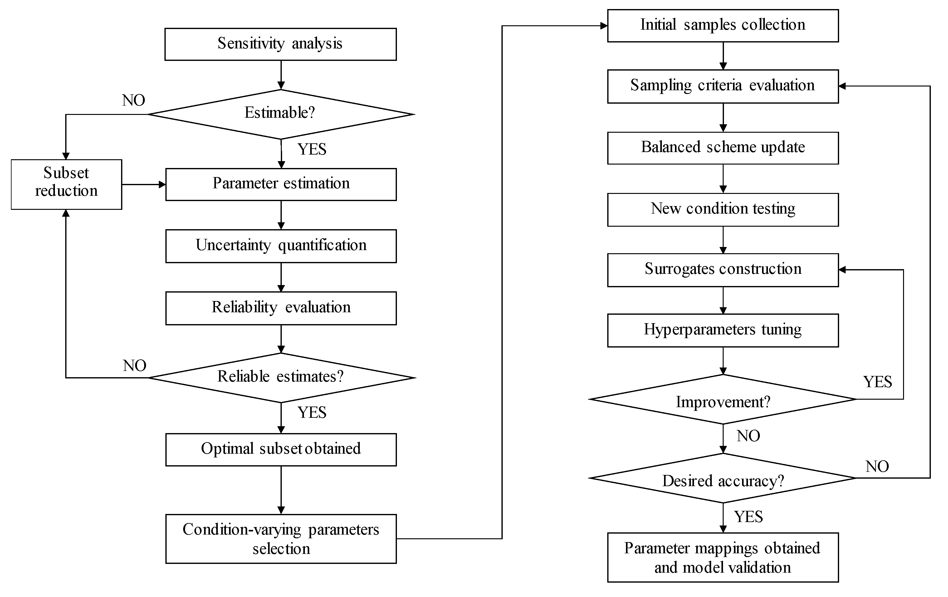
On the basis of the previous discussion, the adaptive model calibration scheme can be summarized as shown in Figure 2. The overall implementation is illustrated below.

Step 1: Sensitivity analysis. Given the original parameter set of the model to be calibrated, local sensitivities at parameter nominal values can be approximated by the barrier sensitivity approach. Estimable parameters are initially selected by the parameter ranking approach.

Step 2: Parameter estimation. Given the process measurements $\tilde{\mathit{w}}$ and the parameter prior distribution $\mathcal{N}\left(\stackrel{-}{\mathit{\theta }},{\mathbf{\Sigma }}_{\theta }\right)$, optimal parameter estimates ${\mathit{\theta }}^{*}$ are obtained by solving the MAP problem as shown in Equation (4).

Step 3: Uncertainty quantification. Parameter uncertainty analysis is developed based on the rMAP approach, which generates approximate samples from the parameter posterior distribution through Monte Carlo experiments of Bayesian estimation. Statistical properties such as the standard deviation and Pearson correlation coefficient can be used to quantify the parameter uncertainty.

Step 4: Reliability evaluation. After uncertainty quantification, reliability factors of the parameters are calculated based on parameter estimates and sample covariance, as shown in Equation (16). The subset is reduced by eliminating the parameters whose estimation results are evaluated as unreliable.

Step 5: Condition-varying parameters selection. Analyze the process principles and select the condition-varying parameters from the optimal subset for global model calibration.

Step 6: Initial samples collection. After specifying the model parameters to be calibrated, several initial samples are required for parameter gradient estimation and surrogate construction. Condition testing is performed for an initial exploration of the design space.

Step 7: Sampling criteria evaluation. When sufficient initial experimental data (sample geometry and corresponding parameter estimates) are collected or a new sample is required, the sampling criteria of sampling density, local nonlinearity and parameter uncertainty of each sample can be measured using Equations (18), (21) and (22), respectively.

Step 8: Balanced scheme update. The balanced scheme is utilized to make a trade-off between exploration and exploitation during the sampling procedure. The hybrid scores are calculated using Equation (23) with a decreasing sequence of the balance parameter $ϵ$. All the samples are ranked based on their hybrid scores.

Step 9: New condition testing. The most undersampled region in the design space is identified by the sample ${\mathit{u}}^k$ with the highest hybrid score. The new experimental condition ${\mathit{u}}^{n_s+1}$ ($n_s$ denotes the current sample size) is placed in the Voronoi cell $v^k$ of ${\mathit{u}}^k$ and kept farthest away from ${\mathit{u}}^k$, together with its ideal neighborhood ${\mathit{U}}_{*}^k$. After conducting condition testing and estimating parameters based on the experimental data, the new sample $\left({\mathit{u}}^{n_s+1},{\mathit{\theta }}^{n_s+1}\right)$ is added into the sample set $\left\{\mathit{U},\mathit{\Theta }\right\}$.

Step 10: Surrogates construction. The SVR surrogates are trained with available experimental samples. Tuning the hyperparameters (e.g., $\epsilon$, $C$ and ${\sigma }_g$) is also a crucial step, since appropriate hyperparameters help ensure surrogate accuracy and prevent overfitting. The SVR surrogates are finally obtained when accuracy improvement no longer occurs. If the desired accuracy of all the surrogates is achieved, the global parameter mappings are completed and it is time to proceed to Step 11. Otherwise, Step 7 should be carried out to select new samples sequentially.

Step 11: Model validation. The global parameter mappings constructed in Step 10 are embedded as parameter submodels into the first principle model. The performance of global model calibration is validated by necessary goodness-of-fit tests.

4. Numerical Results

This section illustrates the application performance of the adaptive model calibration scheme on HTR-PM. The implementation of the algorithm in Section 3.4 can be divided into two stages: parameter subset selection and experimental design of model calibration.

4.1. Parameter Subset Selection

In this subsection, we utilize the systematic parameter estimation approach to select the optimal parameter subset from the 14 thermal hydraulic parameters listed in Table 1 and ensure reliable estimates for further global model calibration.

According to the physical meanings, the parameters in the original set can be categorized into seven types affiliated with the dual NSSS modules. The first four of the seven types are related to the heat transfer process of the nuclear reactor, whereas the latter three describe the thermal characteristics of the steam generator. All the process outputs available for parameter estimation are listed in Appendix A, which is consistent with the arrangement of measuring instruments at the HTR-PM plant site.

Parameter subset selection starts with discussion of the parameter estimability. The local sensitivity of each parameter at its nominal value ${\theta }_i^o$ is approximated by the barrier sensitivity approach and scaled as:

$$\begin{array}{c}{s}_{ik}=\frac{\partial w_k/w_k^o}{\partial {\theta }_i/{\theta }_i^o},i=\mathrm{1,2},\dots ,n_{\theta },k=\mathrm{1,2},\dots ,n_w\end{array}$$

(29)

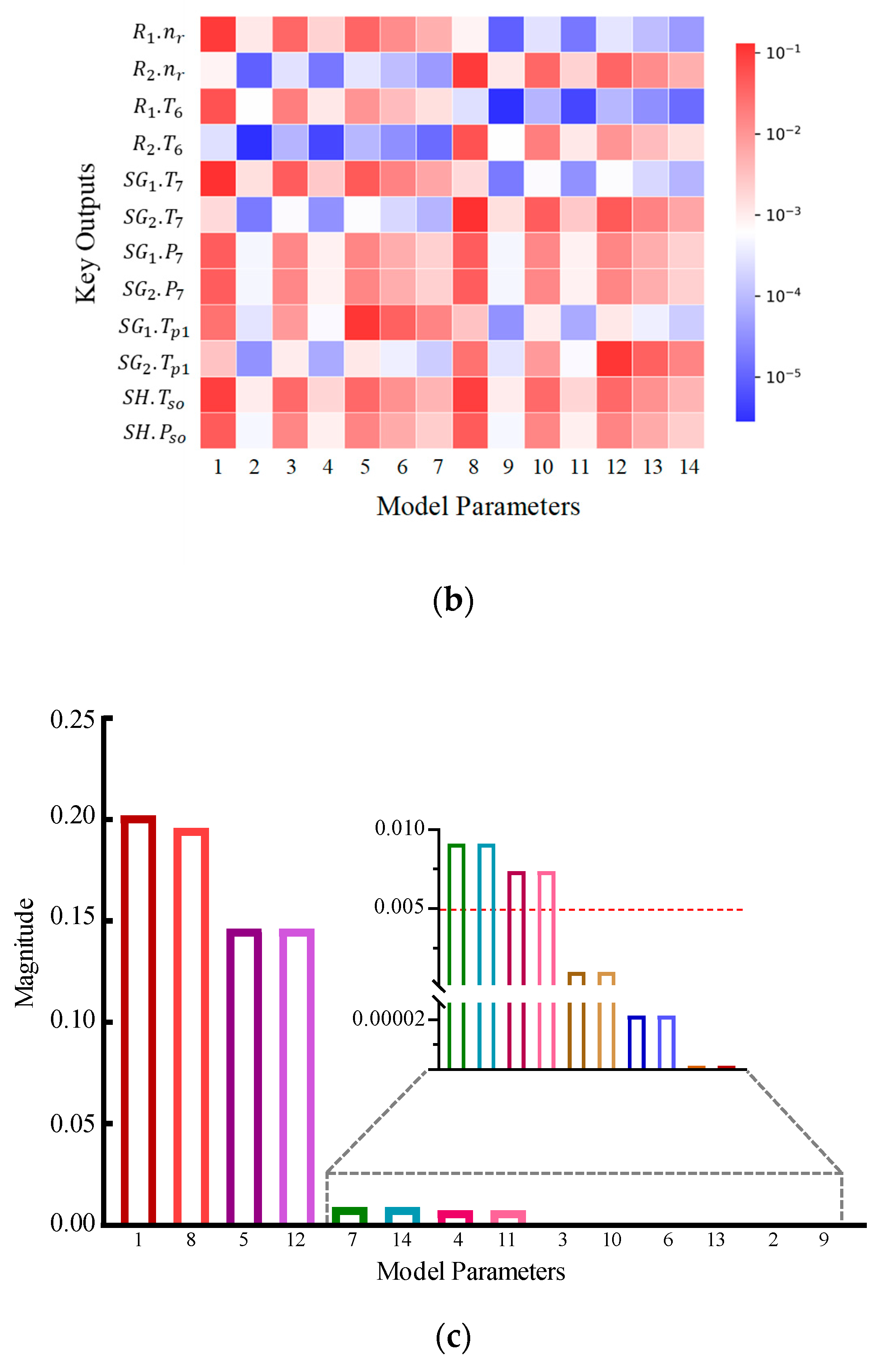
where $s_{ik}$ denotes the kth component of the scaled parameter sensitivity vector ${\mathit{s}}_i$ and $w_k^o$ denotes the model response of output variable $w_k$ at ${\theta }_i^o$. Various experiments have been conducted under different operating conditions of HTR-PM. For convenience of discussion, only sensitivity analysis results under 100%RFP of the dual NSSS modules are demonstrated in this work. The sensitivity vectors of the seven types of parameters are depicted in descending order of magnitude, as shown in Figure 3a. Since relative neutron density, hot/cold helium temperature, steam generator outlet steam temperature/pressure and main steam temperature/pressure are 12 controlled variables of great concern, relevant components of the local sensitivity matrix approximated are illustrated as shown in the heatmap in Figure 3b. Each small square in the heatmap is marked by color to visualize the scaled sensitivity of the controlled variable with respect to the corresponding thermal hydraulic parameter. Red and blue colors represent large and small sensitivity values, respectively. Considering the significant differences between different sensitivities, the specific values of all components in the sensitivity submatrix are depicted in logarithmic form, as indicated by the color bar. The numerical results suggest that the measured outputs of HTR-PM are mainly affected by parameters ${\beta }_2$ and $K_2$. In contrast, the measured outputs are extremely insensitive to variations in parameter ${\alpha }_3{A}_3$, which implies that ${\alpha }_3{A}_3$ may be non-estimable with the available measurements.

On the basis of the parameter sensitivities evaluated, the estimability of the 14 thermal hydraulic parameters is investigated via the parameter ranking approach. Specifically, the Gram–Schmidt orthogonalization process ranks the parameters from the most estimable to the least $\left\{{\beta }_2,K_2,K_6,{\alpha }_{cr}{A}_{cr},{\alpha }_5{A}_5,K_4,{\alpha }_3{A}_3\right\}$. As shown in Figure 3c, the linear correlation between the same type of parameters is relatively weak despite the coupling between the dual NSSS modules. For the predefined threshold ${\rho }_r=0.005$ (as indicated by the red dotted line in Figure 3c), the estimable subset initially selected includes $\left\{{\beta }_2,K_2,K_6,{\alpha }_{cr}{A}_{cr}\right\}$ of each NSSS module.

In addition to estimability analysis, it is also necessary to statistically evaluate the reliability of parameter estimates. The rMAP approach is employed to quantify the parameter uncertainty sourcing from the inherent measurement noise. We first select the sampled operating condition as 100%RFP for the 1# NSSS module and 50%RFP for the 2# NSSS module. The parameter prior density $p\left(\mathit{\theta }\right)$ is assumed in Gaussian distribution. By solving the maximum likelihood estimation (MLE) problem with the given experimental data, the prior mean value $\stackrel{-}{\mathit{\theta }}$ and covariance ${\mathbf{\Sigma }}_{\theta }$ are approximated as the estimated value and the inverse reduced Hessian at the optimal estimated point, respectively. To draw approximate samples from the target parameter posterior distribution, we conduct the Monte Carlo experiments to solve the rMAP problems for 10,000 times with independent random data perturbations. The resulting marginal distributions of the parameter posterior are shown on the diagonal of Figure 4, while the remaining subplots in Figure 4 demonstrate the correlations between the pairwise parameters. On the basis of the sample covariance, the 95% confidence ellipses for each pair of parameters are depicted in the relevant subplots as well. The red dots denote the conditional mean values evaluated for the corresponding parameters.

The Pearson coefficients and the reliability factors defined as Equation (16) are calculated and illustrated in

Table 2. Pearson coefficients between the initially selected parameters.

	$R_1.{\beta }_2$	$R_1.{\alpha }_{cr}{A}_{cr}$	${SG}_1.K_2$	${SG}_1.K_6$	$R_2.{\beta }_2$	$R_2.{\alpha }_{cr}{A}_{cr}$	${SG}_2.K_2$	${SG}_2.K_6$
$R_1.{\beta }_2$	x
$R_1.{\alpha }_{cr}{A}_{cr}$	0.544	x
${SG}_1.K_2$	0.668	0.252	x
${SG}_1.K_6$	−0.061	0.048	−0.404	x
$R_2.{\beta }_2$	−0.095	0.012	0.059	−0.038	x
$R_2.{\alpha }_{cr}{A}_{cr}$	0.014	−0.003	0.001	−0.011	0.617	x
${SG}_2.K_2$	0.068	−0.008	−0.018	−0.036	0.423	0.268	x
${SG}_2.K_6$	−0.050	0.006	0.011	0.049	−0.021	0.010	−0.755	x

and

Table 3. Reliability factors of the initially selected parameters.

${\theta }_i$	$R_1.{\beta }_2$	$R_1.{\alpha }_{cr}{A}_{cr}$	${SG}_1.K_2$	${SG}_1.K_6$	$R_2.{\beta }_2$	$R_2.{\alpha }_{cr}{A}_{cr}$	${SG}_2.K_2$	${SG}_2.K_6$
$r_i$	0.0042	0.0750	0.0096	0.0359	0.0052	0.0653	0.0181	0.1280

, respectively. The results prove that there is no strong linear correlation among the initially selected parameters since the non-estimable parameters have already been eliminated. However, parameters ${\alpha }_{cr}{A}_{cr}$ and $K_6$ exhibit significant uncertainty due to high standard deviations. Their reliability factors exceed the predefined threshold ${\rho }_f=0.02$, which indicates that the estimation results of these parameters are evaluated as unreliable. The optimal parameter subset for reliable estimation is finally refined to $\left\{{\beta }_2,K_2\right\}$.

4.2. Global Model Calibration of HTR-PM

According to the process principles, although the parameters ${\beta }_2$ in the optimal subset have the most significant effects on various model outputs, such parameters will only evolve slowly with long-term operations of the nuclear system. This type of time-varying parameter remains relatively consistent over the global operating domain. Conversely, there is a positive correlation between the parameters $K_2$ and the system load since the increase in thermal load signifies the increase in heat flux density in each section of the steam generator. This subsection is devoted to calibration of the parameter $K_2$ over global operating domain.

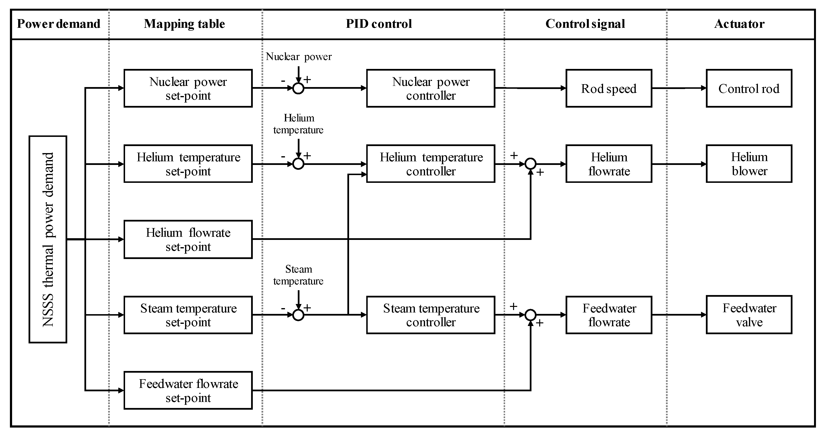
The global parameter mapping is built through the manipulated variables $\mathit{u}$, which include external reactivity, helium flow rate, feedwater flow rate and opening of the main steam regulating valve for the HTR-PM plant. Load change operations of the nuclear system are carried out based on the coordinated PID control scheme shown in Figure 5. Under this control scheme, each manipulated variable is determined by the thermal power demand of the dual NSSS modules and the look-up table method [38]. Hence, we can reduce the design space from seven-dimensional to two-dimensional (i.e., 1# PowerDemand and 2# PowerDemand) for convenience of discussion. It is noteworthy that only thermal power demand from 50% RFP to 100% RFP is studied, whereas special scenarios such as shutdown and accidents are not our concern.

The global model calibration experiments start with collection of the initial samples. Considering the particular requirements of the LOLA algorithm for gradient estimation, we need at least $2n_u+1=5$ condition samples to initialize our experimental design. To obtain preliminary insights into the parameter behavior over the global operating domain, the initial samples are generated to evenly fill up the design space as $\left\{\left(0.74,0.76\right),\left(0.50,0.655\right),\left(0.68,0.51\right),\left(0.98,0.80\right),\left(0.78,0.995\right)\right\}$. Under each sampled condition, parameter estimation is performed based on the process measurements. Sampling criteria of sampling density, local nonlinearity and parameter uncertainty are evaluated using the Voronoi tessellation, LOLA and uncertainty quantification techniques, respectively. The existing samples are ranked in descending order according to the hybrid score consisting of the three measures. Since a high hybrid score may derive from sparse sampling, strong nonlinearity and significant parameter uncertainty, the new experimental condition is selected in the vicinity of the sample with the highest hybrid score.

The adaptive experimental design of model calibration proposed is essentially a generic and surrogate-independent approach. Here, we utilize different kinds of surrogates to construct the data-driven parameter mappings with the same initial samples. In addition to SVR, other surrogate types for comparison include kriging interpolation with exponential correlation (Kriging), linear regression (LR) and quadratic approximation (QA) [30].

Sample ranking, condition testing, parameter estimation and surrogate construction are alternately repeated until the surrogate accuracy achieves the expectation. The experimental results of global model calibration based on different surrogates are shown in Figure 6. The Voronoi diagrams on the left column illustrate the sample distribution in the design space. With the same initial samples and measurement noise level, the sampling procedures based on SVR, QA, Kriging and LR surrogates end with 11, 14, 19 and 19 experiments, respectively. In the Voronoi diagrams, larger blue dots represent higher parameter uncertainty evaluated. It can be intuitively observed that the uncertainty of the parameter $K_2$ increases when the NSSS module is operating under a low load condition, and the algorithm therefore tends to drive sampling to this region. The surrogate accuracy is validated by calculating the relative prediction errors over the design space and shown in the heatmap on the right. The SVR surrogates outperform other surrogates in both the number of experiments and global prediction accuracy. The maximum relative errors of the parameters predicted by the SVR surrogates are as low as 0.35% and 0.36%. Despite the equally satisfying accuracy provided by the QA surrogate, it requires at least $\frac{\left(n_u+1\right)\left(n_u+2\right)}{2}$ samples to determine the regression coefficients, which is obviously unsuitable for high-dimensional input cases. Considering the strict safety standards and high experimental cost of the HTR-PM plant, we highlight the effectiveness of SVR in small sample learning.

We compare the proposed adaptive model calibration scheme with conventional techniques based on static experimental designs. All the model calibration experiments employ SVR with the Gaussian kernel as the global surrogate of parameter mapping. The static experimental designs include grid sampling, Latin hypercube sampling (LHS, classic LHS and centered LHS) and low-discrepancy sequences (Sobol, Halton and Hammersley) [23]. Except for the grid design, which samples 16 experimental conditions, all the other designs select 12 experimental conditions for global model calibration. For each experimental design, the SVR surrogates are constructed based on the corresponding samples. The resulting SVR surrogates’ relative prediction errors over the design space are shown in Figure 7. The black dots in each heatmap represent the experimental conditions determined by the corresponding experimental design. Our adaptive model calibration scheme mainly outperforms the static techniques in two aspects. On the one hand, the static techniques focus on evenly filling the design space and cannot utilize the system response, whereas the adaptive scheme can identify the irregular regions of parameter behavior by information of parameter nonlinearity and uncertainty. On the other hand, static experimental design is essentially a one-shot approach, which may lead to oversampling or undersampling in practice. On the contrary, the adaptive scheme based on a sequential design can make flexible adjustments to the system response and end the sampling procedure in time once the parameter mappings are precise enough. Consequently, the adaptive model calibration scheme achieves higher parameter prediction accuracy over the global operating domain (the maximum relative errors of the globally calibrated parameters ${SG}_1.K_2$ and ${SG}_2.K_2$ are as low as 0.35% and 0.36%, respectively) through fewer trials (only 11 condition experiments are conducted), which is meaningful for the safety and economy of the HTR-PM plant.

5. Conclusions and Future Work

Process control and optimization based on first principle models are the pivotal technologies to ensure safe and efficient operation of the innovative HTR-PM plant, and reliable decisions must come from models that can accurately describe the operating characteristics of the nuclear system. To identify the thermal hydraulic parameters of HTR-PM over the global operating domain with modest experimental cost, an adaptive model calibration scheme is designed in this work. First, a data-driven parameter mapping is presented to enable global model calibration. We then discuss the estimability and uncertainty of the model parameters via sensitivity analysis and reliability evaluation. The optimal parameter subset with reliable estimates is determined through a heuristic subset reduction procedure. To solve the conflicts between high prediction accuracy and low operating cost when constructing parameter mapping, an adaptive experimental design that comprehensively considers sampling density, local nonlinearity and parameter uncertainty is adopted for model calibration. Finally, adaptive model calibration is fulfilled by combining the small-sample learning quality of the SVR surrogate. As demonstrated by the simulation results, the thermal hydraulic parameters that can be estimated simultaneously are the helium leakage ratio inside the reactor and the overall heat transfer coefficient of the preheated section in the steam generator. In addition to the optimal parameter estimates, the parameter uncertainty is quantified by inferring the parameter posterior distributions, which effectively evaluate the reliability of the resulting estimates. The adaptive model calibration scheme outperforms the conventional techniques (based on static experimental designs) in both the number of experiments and global prediction accuracy. On the one hand, the adaptive experimental design makes a trade-off between exploration and exploitation, which enables the sampling procedure to identify the irregular regions of parameter behavior while filling up the design space. On the other hand, the sequential design ends in time once the SVR-based parameter mappings achieve the desired accuracy, and potential issues with oversampling and undersampling are effectively excluded. Consequently, the adaptive model calibration scheme can obtain high global calibration accuracy of model parameters with low experimental cost.

On the basis of this work, the following aspects will be studied in our future research:

(1) Global model calibration of HTR-PM explores the parameter behavior over the global operating domain. In practice, the time-varying characteristic of parameters is another source of uncertainty. We will extend the algorithm to support the calibration of time-varying parameters.

(2) To ensure the reliability of parameter estimates and improve the observability of nuclear systems, the possibility of sensor network redesign by parameter estimability analysis is under investigation.

(3) The HTR-PM plant has been formally connected to the electrical grid and will further conduct trial operations of load change. Future work will focus on practical applications of the adaptive model calibration scheme.

References

1. Locatelli, G.; Mancini, M.; Todeschini, N. Generation IV Nuclear Reactors: Current Status and Future Prospects. Energy Policy 2013, 61, 1503–1520. [Google Scholar] [CrossRef]
2. Nian, V. Technology Perspectives from 1950 to 2100 and Policy Implications for the Global Nuclear Power Industry. Prog. Nucl. Energy 2018, 105, 83–98. [Google Scholar] [CrossRef]
3. Wu, Z.; Lin, D.; Zhong, D. The Design Features of the HTR-10. Nucl. Eng. Des. 2002, 218, 25–32. [Google Scholar] [CrossRef]
4. Zhang, Z.; Dong, Y.; Li, F.; Zhang, Z.; Wang, H.; Huang, X.; Li, H.; Liu, B.; Wu, X.; Wang, H.; et al. The Shandong Shidao Bay 200 MWe High-Temperature Gas-Cooled Reactor Pebble-Bed Module (HTR-PM) Demonstration Power Plant: An Engineering and Technological Innovation. Engineering 2016, 2, 112–118. [Google Scholar] [CrossRef] [Green Version]
5. Xu, S.; Lu, Y.; Mutailipu, M.; Yan, K.; Zhang, Y.; Qvist, S. Repowering Coal Power in China by Nuclear Energy—Implementation Strategy and Potential. Energies 2022, 15, 1072. [Google Scholar] [CrossRef]
6. Gu, Z. History Review of Nuclear Reactor Safety. Ann. Nucl. Energy 2018, 120, 682–690. [Google Scholar] [CrossRef]
7. Oettingen, M.; Cetnar, J. Numerical Modelling of Modular High-Temperature Gas-Cooled Reactors with Thorium Fuel. Nukleonika 2021, 66, 133–138. [Google Scholar] [CrossRef]
8. Kępisty, G.; Oettingen, M.; Stanisz, P.; Cetnar, J. Statistical Error Propagation in HTR Burnup Model. Ann. Nucl. Energy 2017, 105, 355–360. [Google Scholar] [CrossRef]
9. Dong, Z.; Cheng, Z.; Zhu, Y.; Huang, X.; Dong, Y.; Zhang, Z. Review on the Recent Progress in Nuclear Plant Dynamical Modeling and Control. Energies 2023, 16, 1443. [Google Scholar]
10. Zhang, Z.; Ye, P.; Yang, X.T.; Ju, H.M.; Jiang, S.Y.; Tu, J.Y. Supercritical Steam Generator Design and Thermal Analysis Based on HTR-PM. Ann. Nucl. Energy 2019, 132, 311–321. [Google Scholar] [CrossRef]
11. Dong, Z. Saturated Adaptive Output-Feedback Power-Level Control for Modular High Temperature Gas-Cooled Reactors. Energies 2014, 7, 7620–7639. [Google Scholar] [CrossRef] [Green Version]
12. Du, X.; Ma, X.; Liu, J.; Wu, S.; Wang, P. Operation Optimization of Auxiliary Electric Boiler System in HTR-PM Nuclear Power Plant. Nucl. Eng. Technol. 2022, 54, 2840–2851. [Google Scholar] [CrossRef]
13. Carlos, S.; Ginestar, D.; Martorell, S.; Serradell, V. Parameter Estimation in Thermalhydraulic Models Using the Multidirectional Search Method. Ann. Nucl. Energy 2003, 30, 133–158. [Google Scholar] [CrossRef]
14. Zio, E.; Zoia, A. Bayesian Inference of BWR Model Parameters by Markov Chain Monte Carlo. Ann. Nucl. Energy 2008, 35, 1929–1936. [Google Scholar] [CrossRef]
15. Fazekas, C.; Szederkényi, G.; Hangos, K.M. Parameter Estimation of a Simple Primary Circuit Model of a VVER Plant. IEEE Trans. Nucl. Sci. 2008, 55, 2643–2653. [Google Scholar] [CrossRef]
16. Wu, Y.; Ren, C.; Li, R.; Yang, X.; Tu, J.; Jiang, S. Method and Validation for Measurement of Effective Thermal Diffusivity and Conductivity of Pebble Bed in High Temperature Gas-Cooled Reactors. J. Nucl. Eng. Radiat. Sci. 2018, 4, 133–158. [Google Scholar] [CrossRef]
17. Mclean, K.A.P.; Mcauley, K.B. Mathematical Modelling of Chemical Processes-Obtaining the Best Model Predictions and Parameter Estimates Using Identifiability and Estimability Procedures. Can. J. Chem. Eng. 2012, 90, 351–366. [Google Scholar] [CrossRef]
18. Kravaris, C.; Hahn, J.; Chu, Y. Advances and Selected Recent Developments in State and Parameter Estimation. Comput. Chem. Eng. 2013, 51, 111–123. [Google Scholar] [CrossRef]
19. Nakama, C.S.M.; Le Roux, G.A.C.; Zavala, V.M. Optimal Constraint-Based Regularization for Parameter Estimation Problems. Comput. Chem. Eng. 2020, 139, 106873. [Google Scholar] [CrossRef]
20. Lund, B.F.; Foss, B.A. Parameter Ranking by Orthogonalization-Applied to Nonlinear Mechanistic Models. Automatica 2008, 44, 278–281. [Google Scholar] [CrossRef]
21. Chen, W.; Biegler, L.T. Reduced Hessian Based Parameter Selection and Estimation with Simultaneous Collocation Approach. AIChE J. 2020, 66, e16242. [Google Scholar] [CrossRef]
22. Marsili-Libelli, S.; Guerrizio, S.; Checchi, N. Confidence Regions of Estimated Parameters for Ecological Systems. Ecol. Model. 2003, 165, 127–146. [Google Scholar] [CrossRef]
23. Garud, S.S.; Karimi, I.A.; Kraft, M. Design of Computer Experiments: A Review. Comput Chem Eng 2017, 106, 71–95. [Google Scholar] [CrossRef]
24. Kim, J.H.; Lee, J.M. Efficient Online Model-Based Design of Experiments via Parameter Subset Selection for Batch Dynamical Systems. Comput. Chem. Eng. 2019, 121, 646–653. [Google Scholar] [CrossRef]
25. Jung, Y.; Lee, I. Optimal Design of Experiments for Optimization-Based Model Calibration Using Fisher Information Matrix. Reliab. Eng. Syst. Saf. 2021, 216, 107968. [Google Scholar] [CrossRef]
26. Li, H.; Huang, X.; Zhang, L. A Simplified Mathematical Dynamic Model of the HTR-10 High Temperature Gas-Cooled Reactor with Control System Design Purposes. Ann. Nucl. Energy 2008, 35, 1642–1651. [Google Scholar] [CrossRef]
27. Li, H.; Huang, X.; Zhang, L. A Lumped Parameter Dynamic Model of the Helical Coiled Once-through Steam Generator with Movable Boundaries. Nucl. Eng. Des. 2008, 238, 1657–1663. [Google Scholar] [CrossRef]
28. Yang, C.; Wang, K.; Shao, Z.; Biegler, L.T. Integrated Parameter Mapping and Real-Time Optimization for Load Changes in High-Temperature Gas-Cooled Pebble Bed Reactors. Ind. Eng. Chem. Res. 2018, 57, 9171–9184. [Google Scholar] [CrossRef]
29. Conn, A.R.; Scheinberg, K.; Vicente, L.N. Geometry of Interpolation Sets in Derivative Free Optimization. Math. Program. 2008, 111, 141–172. [Google Scholar] [CrossRef] [Green Version]
30. Bhosekar, A.; Ierapetritou, M. Advances in Surrogate Based Modeling, Feasibility Analysis, and Optimization: A Review. Comput. Chem. Eng. 2018, 108, 250–267. [Google Scholar] [CrossRef]
31. Pirnay, H.; López-Negrete, R.; Biegler, L.T. Optimal Sensitivity Based on IPOPT. Math. Program. Comput. 2012, 4, 307–331. [Google Scholar] [CrossRef]
32. Wächter, A.; Lorenz, T.; Biegler, T. On the Implementation of an Interior-Point Filter Line-Search Algorithm for Large-Scale Nonlinear Programming. Math. Program. 2006, 106, 25–57. [Google Scholar] [CrossRef]
33. Wang, K.; Bui-Thanh, T.; Ghattas, O. A Randomized Maximum a Posteriori Method for Posterior Sampling of High Dimensional Nonlinear Bayesian Inverse Problems. SIAM J. Sci. Comput. 2018, 40, A142–A171. [Google Scholar] [CrossRef]
34. Shin, S.; Venturelli, O.S.; Zavala, V.M. Scalable Nonlinear Programming Framework for Parameter Estimation in Dynamic Biological System Models. PLoS Comput. Biol. 2019, 15, e1006828. [Google Scholar] [CrossRef] [Green Version]
35. Crombecq, K.; Gorissen, D.; Deschrijver, D.; Dhaene, T. A Novel Hybrid Sequential Design Strategy for Global Surrogate Modeling of Computer Experiments. SIAM J. Sci. Comput. 2011, 33, 1948–1974. [Google Scholar] [CrossRef]
36. Smola, A.J.; Schölkopf, B. A Tutorial on Support Vector Regression. Stat. Comput. 2004, 14, 199–222. [Google Scholar] [CrossRef] [Green Version]
37. Ruiz, C.; Alaíz, C.M.; Dorronsoro, J.R. Multitask Support Vector Regression for Solar and Wind Energy Prediction. Energies 2020, 13, 6308. [Google Scholar] [CrossRef]
38. Jiang, D.; Dong, Z. Dynamic Matrix Control for Thermal Power of Multi-Modular High Temperature Gas-Cooled Reactor Plants. Energy 2020, 198, 117386. [Google Scholar] [CrossRef]
Figure 1. First principle modeling of the HTR-PM plant. (a) Schematic diagram of the HTR-PM plant. (b) Schematic diagram of the HTR-PM model.
Energies 16 04653 g001aEnergies 16 04653 g001b
Figure 2. Algorithm procedure of adaptive model calibration scheme.
Energies 16 04653 g002
Figure 3. Initial parameter subset selection via sensitivity analysis. (a) Magnitudes of parameter sensitivity vectors. (b) Local sensitivity submatrix approximated at 100%RFP. (c) Parameter ranking and estimable subset selection.
Energies 16 04653 g003aEnergies 16 04653 g003b
Figure 4. Uncertainty quantification results of parameter posterior distributions.
Energies 16 04653 g004
Figure 5. Coordinated PID control scheme of the HTR-PM plant.
Energies 16 04653 g005
Figure 6. Global model calibration of HTR-PM based on different types of surrogates.
Energies 16 04653 g006
Figure 7. Global model calibration of HTR-PM based on different experimental designs.
Energies 16 04653 g007