Modelling Electro-Mechanical Behaviour of an XLPE Insulation Layer for Hi-Voltage Composite Power Cables: Effect of Voids on Onset of Coalescence

Abstract

The harshness of the submarine environment represents a serious threat for immersed high voltage power cables, extensively used for offshore wind farms, which in turn are supposed to last for at least 20 years for their total investment to be economically viable. The Crosslinked Polyethylene (XLPE) used for the insulating layer of the cables may suffer different degradation phenomena, leading to unexpected breakdowns and rises in costs. In this work, numerical simulations have been developed to study the mechanisms by which micrometric pores inside XLPE can enlarge and coalesce (namely, water treeing) when the insulation is subjected to the intense electric field generated by hi-voltage wires. The study aim is to predict material plasticization next to voids, which is supposed to represent the onset of coalescence of neighboring pores. A microscale-level finite element coupled electro-mechanics model has been developed to describe the interactions between the intense electric fields and the subsequent Maxwell stresses in a dielectric. The roles of different influencing parameters such as distance, relative volumes, and the shape of two neighboring voids in a representative unit volume are considered. Finally, the behavior of a generic microstructure characterized by randomly distributed voids immersed in an electric field is simulated.

1. Introduction

Crosslinked Polyethylene (XLPE) is one of the most versatile dielectrics on the market [1]. Thanks to its outstanding mechanical and electrical properties, it has been widely used in the field of electric cable insulation since the early 1960s [2]. One of its most demanding applications nowadays is represented by the insulation of submerged high voltage cables that are needed for offshore wind farms. The harshness of the marine environment (i.e., high thermal gradients, presence of moisture with consequent dissolved ionic species) and the hi-voltage electric fields are of considerable concern for the renewable energies industry, with huge potential economic losses in case of power transmission system breakdowns. Although XLPE is still considered the most suitable insulator for dealing with these extreme conditions, the electrical lifetime of this insulation is greatly reduced in these conditions; this results in a considerable degradation of the cables after only 5–10 years of service, instead of an expected service life of 20–30 years [3]. The typical risk associated with prolonged service life inside submerged environments is water treeing [2]—a degradation phenomenon in which small, permanent, water-filled voids form inside the XLPE, causing a sharp reduction in the breakdown voltage (i.e., the minimum voltage that causes local portions of the insulator to become electrically conductive). In the literature [4,5], it has been demonstrated that mechanical fatigue (caused by dielectrophoretic stress around the voids) is the main reason for water treeing. Fatigue can easily arise from shipping, handling and immersing cables in deep seas, which may cause excess plasticity in the weakest XPLE areas. Due to differences in the dielectric constant of water and XLPE, non-uniform electric fields develop around the pores. Additionally, the development of such electric fields causes the evolution of spherical voids into ellipsoidal-shaped cavities due to the polarization effect. These ellipsoidal cavities have high electric fields and resultant Maxwell stresses at the tips. It was evidenced in [6] that electric fields of up to 50 kV/mm do not cause plastic deformation, whereas in [7], it has been shown how fields beyond 100 kV/mm can cause permanent deformation of voids. After several years, alternating electric fields associated with the AC current lead to tree growth and the formation of channels between voids. Water can freely propagate in the channels towards the conductor, triggering corrosion and the ultimate failure of the cable. 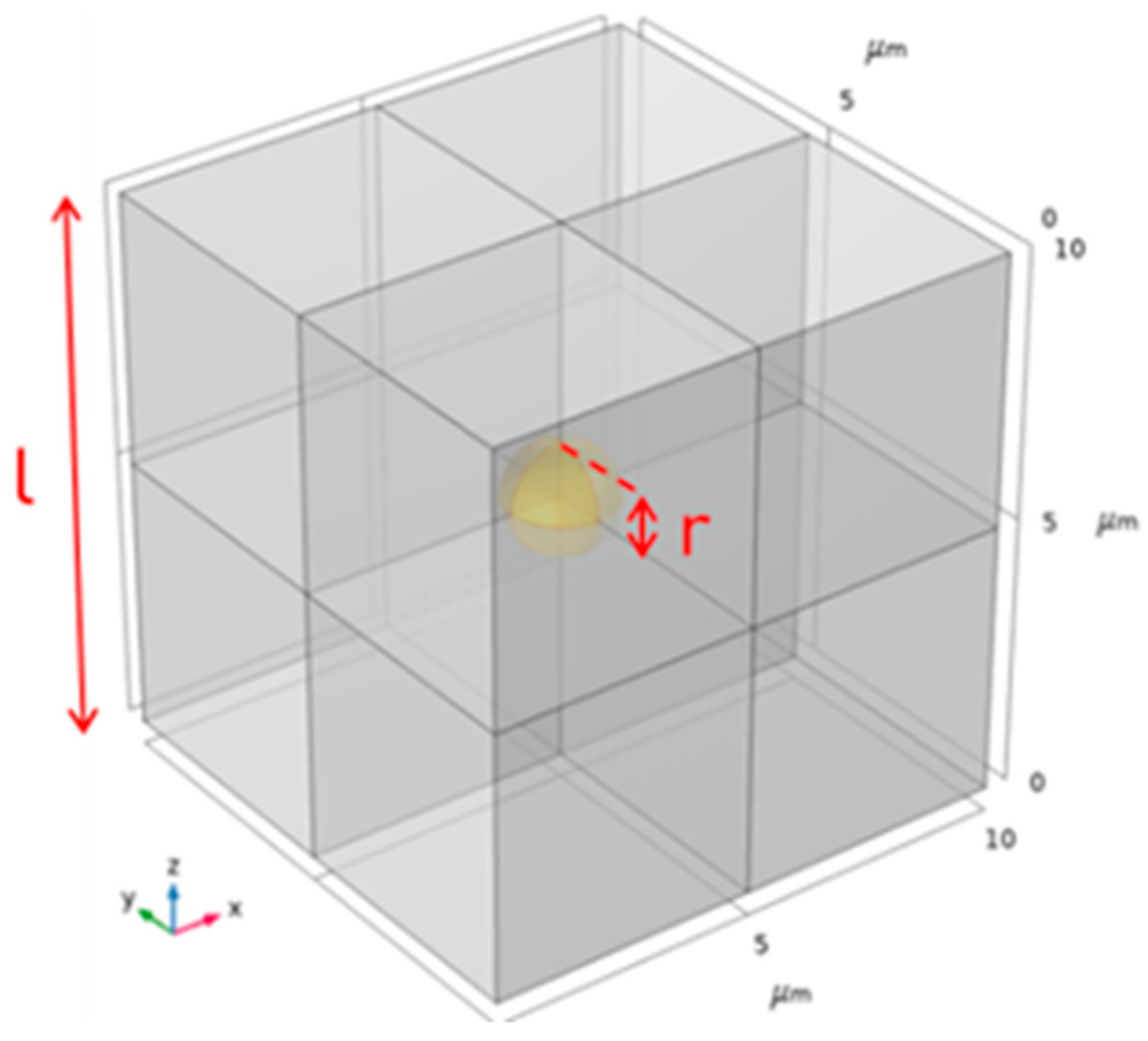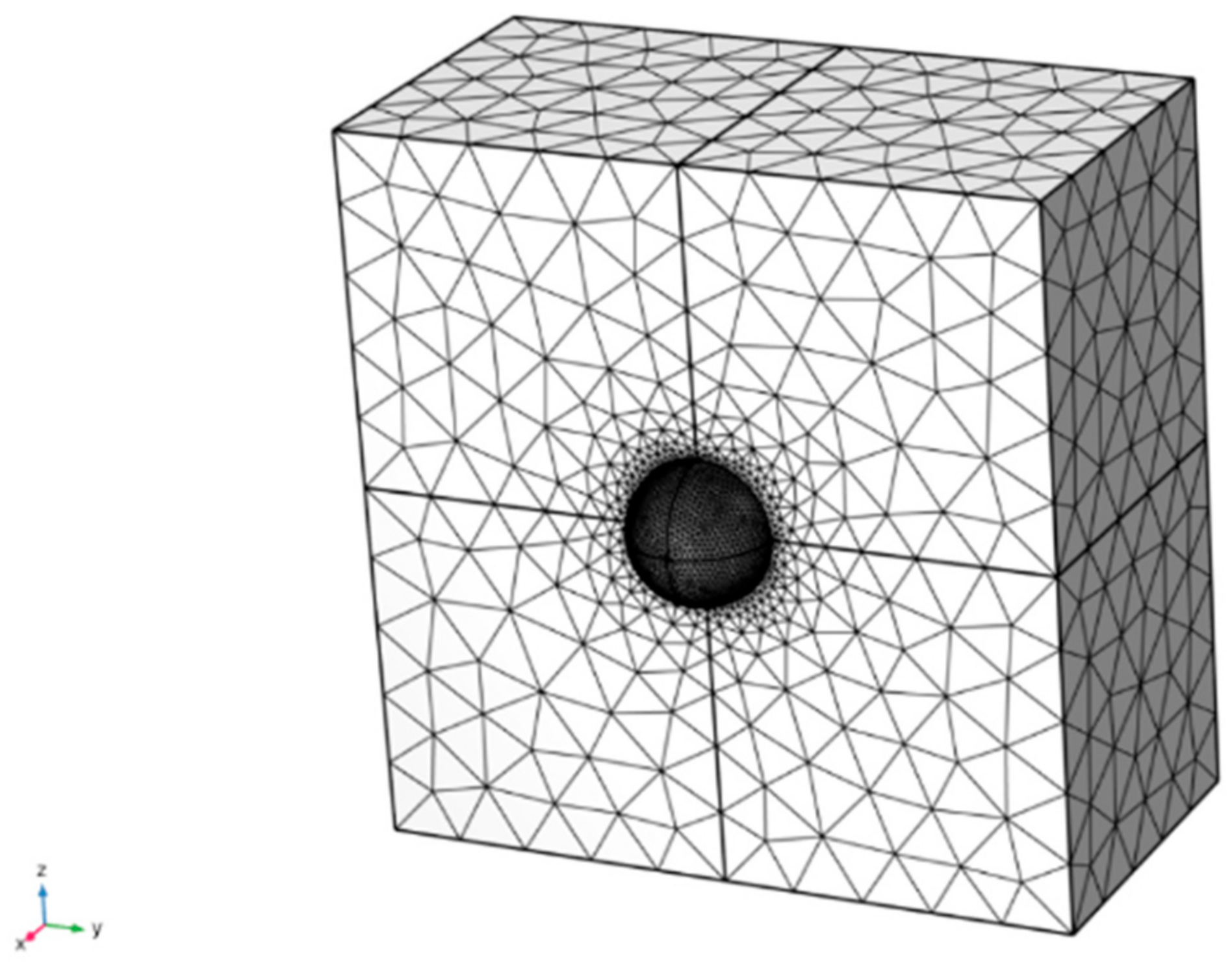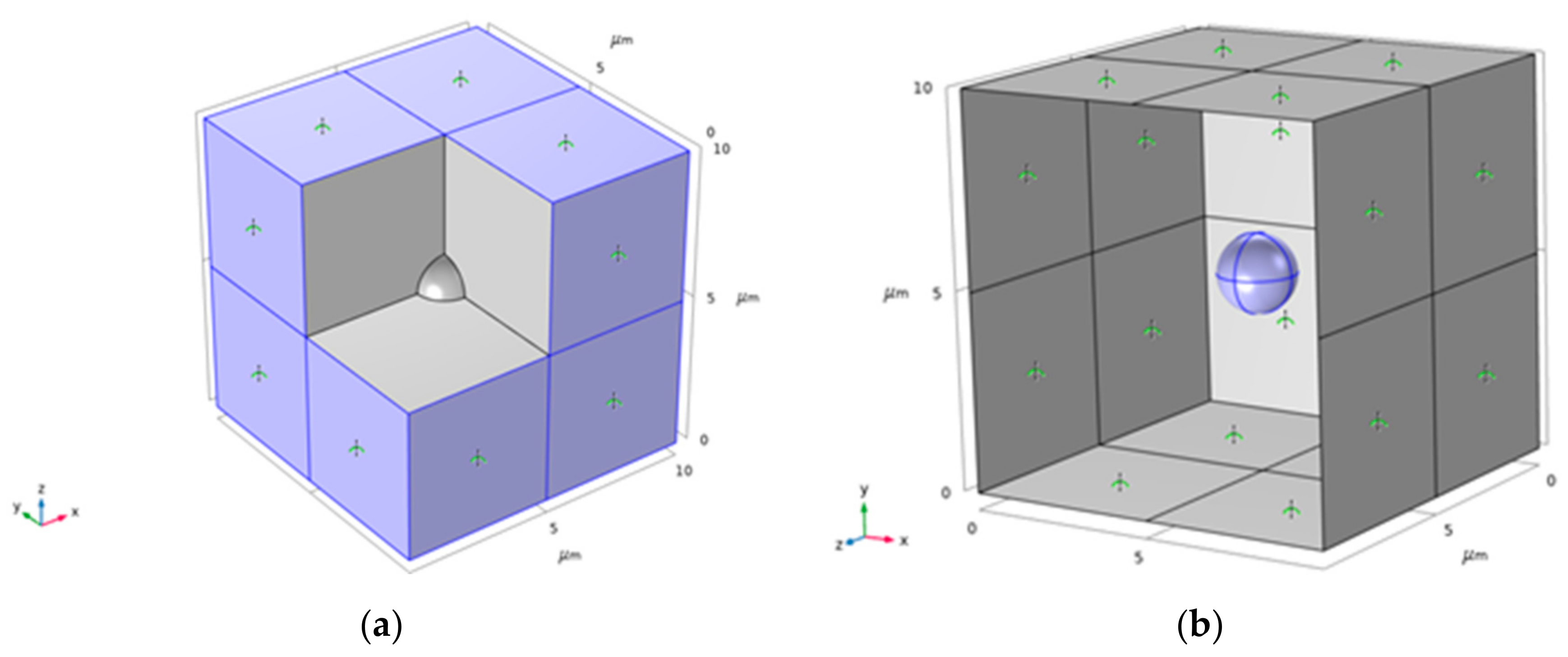Therefore, lot of research has been conducted on this topic to better understand the mechanisms by which treeing occurs [2], as well as appropriate structural health monitoring concepts to account for phase over-strain [8]. In the literature, the most commonly adopted approach to this problem is predictive models, avoiding complex, expensive, and time-consuming experimental testing campaigns that may last for decades. On one hand, although accelerated laboratory tests do exist, these do not ensure that the polymeric materials have the actual morphology and properties that stem from a long service life in a submarine environment. On the other hand, using Multiphysics FEM models, it is possible to simulate the XLPE microstructure (characterized by the presence of defects and pores, from the manufacturing stage) and its response to electrical stimuli, obtaining reliable results at different scales. The simulation of the entire microstructure’s behavior is unfeasible; hence, the macroscopic equivalent behavior can be predicted by studying a representative volume element (RVE), assuming a periodic distribution of the voids in the material. 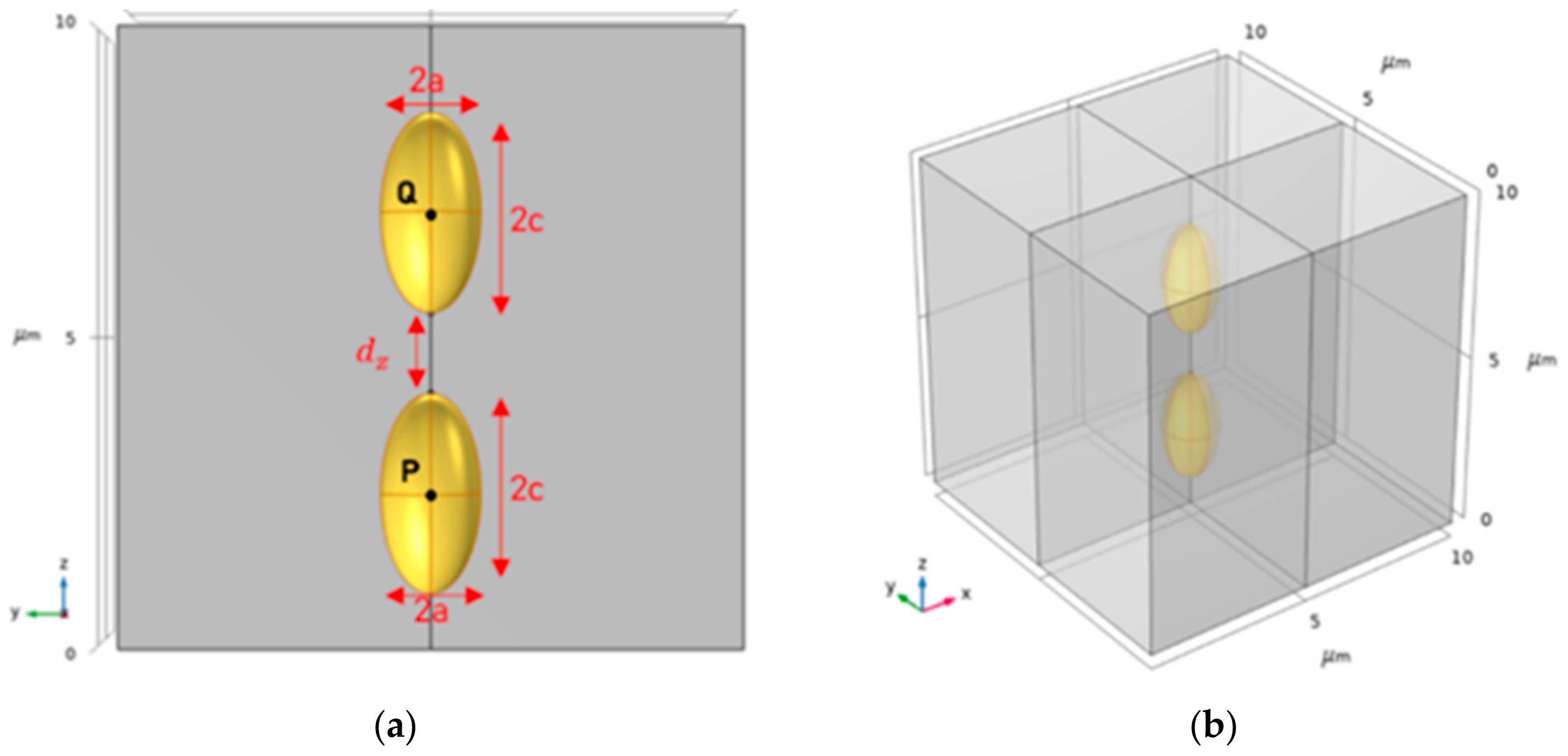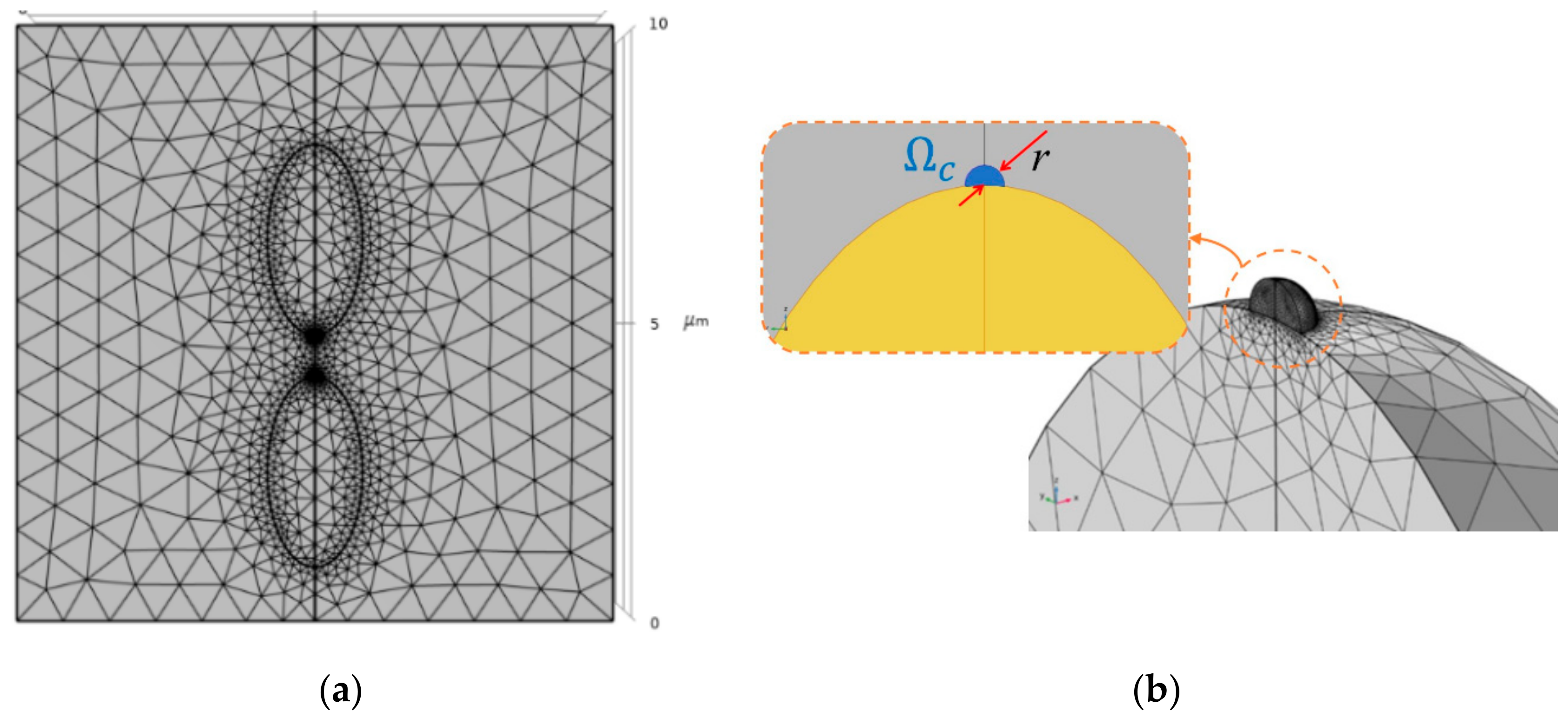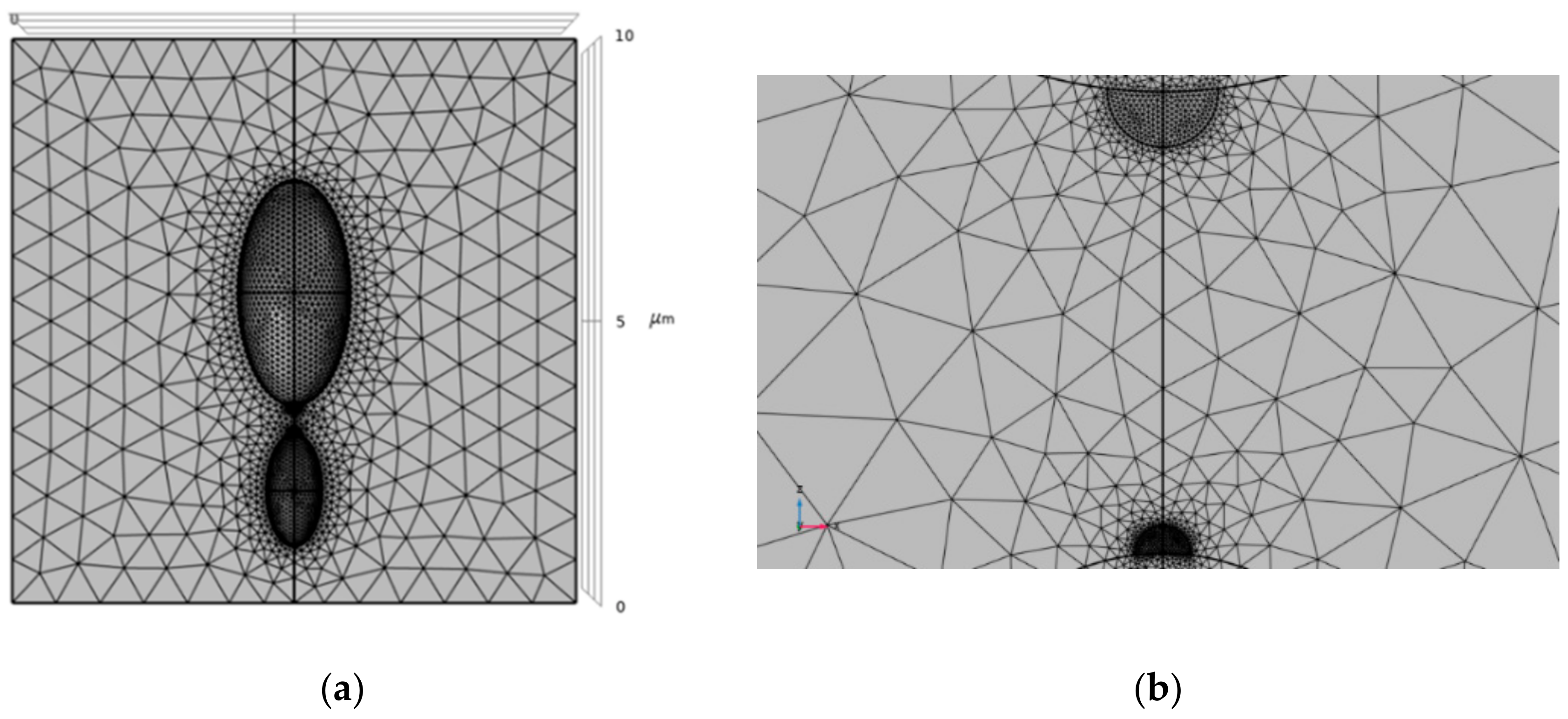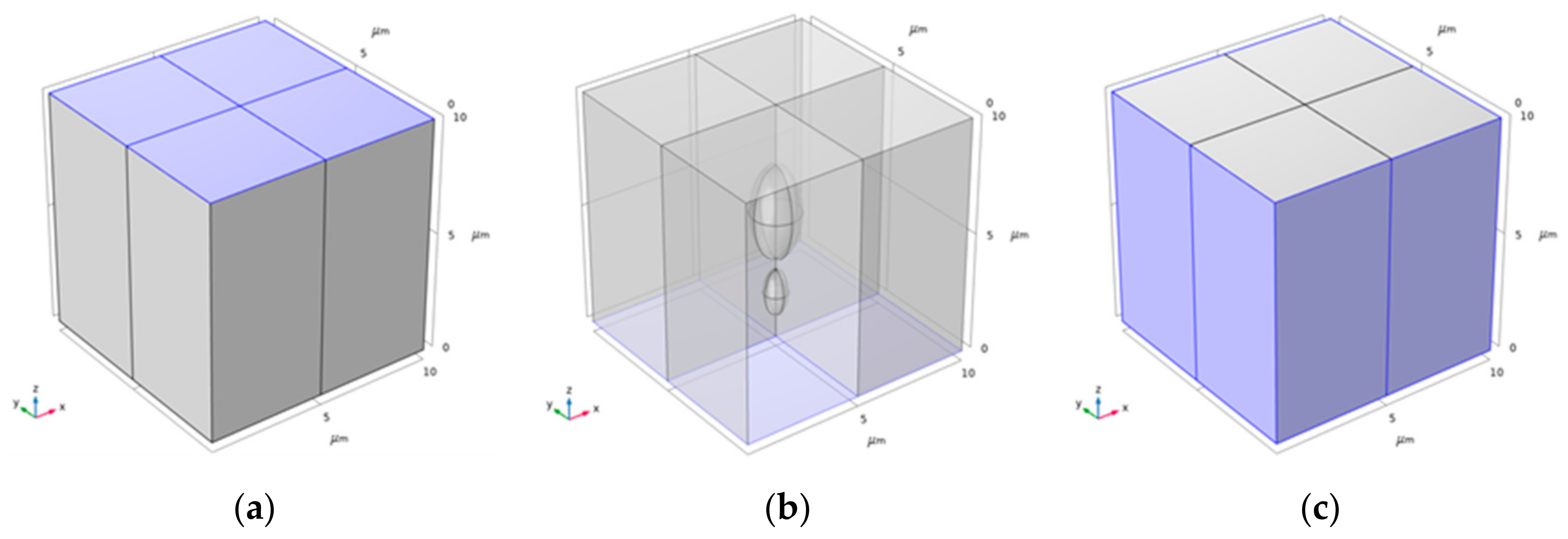In [8], RVE has been exploited to study the pores’ deformation, leading to ellipsoids due to the polarization effect; intense electric fields and Maxwell stresses generate at the void tips, causing polymer yielding and coalescence between different pores. The deformation and material yielding around two ellipsoidal water-filled voids in a cubic RVE subjected to an intense electric field have been examined, and the effect of different geometrical variables such as orientation and number of voids has been predicted [3,8]. The static electric field has been considered, neglecting the alternating behavior of the AC current and fatigue degradation due to cyclic loading and unloading.

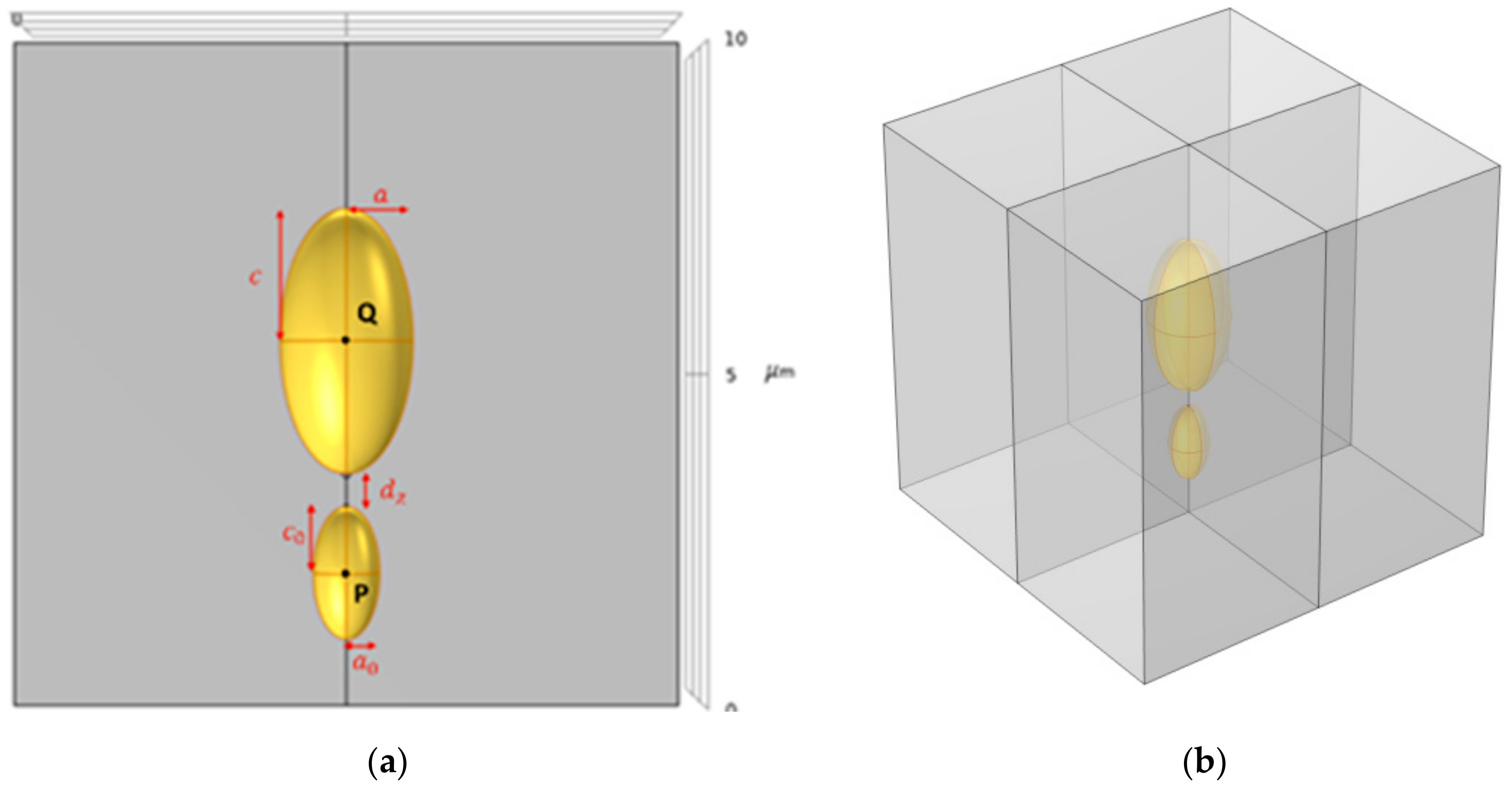
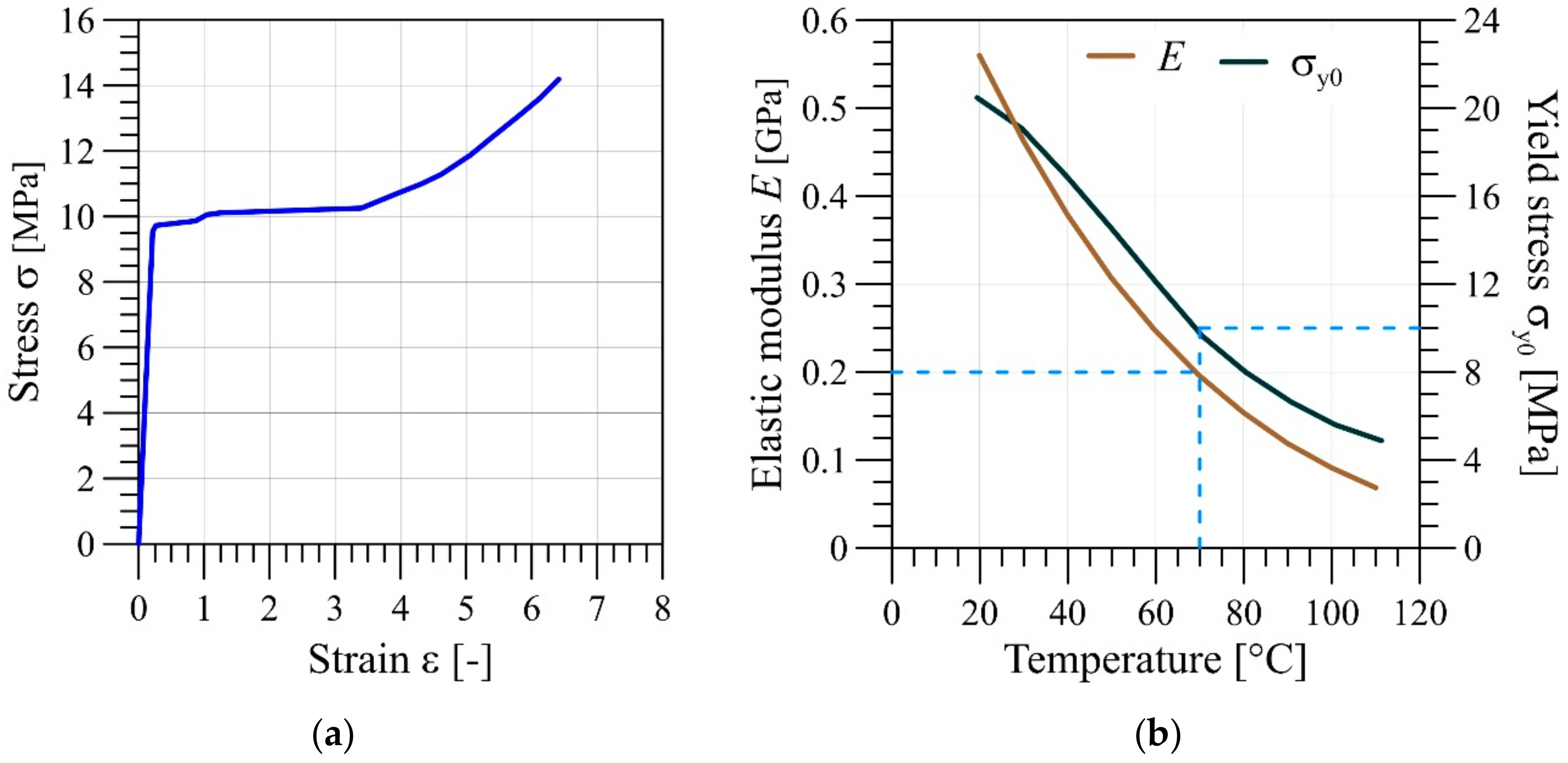
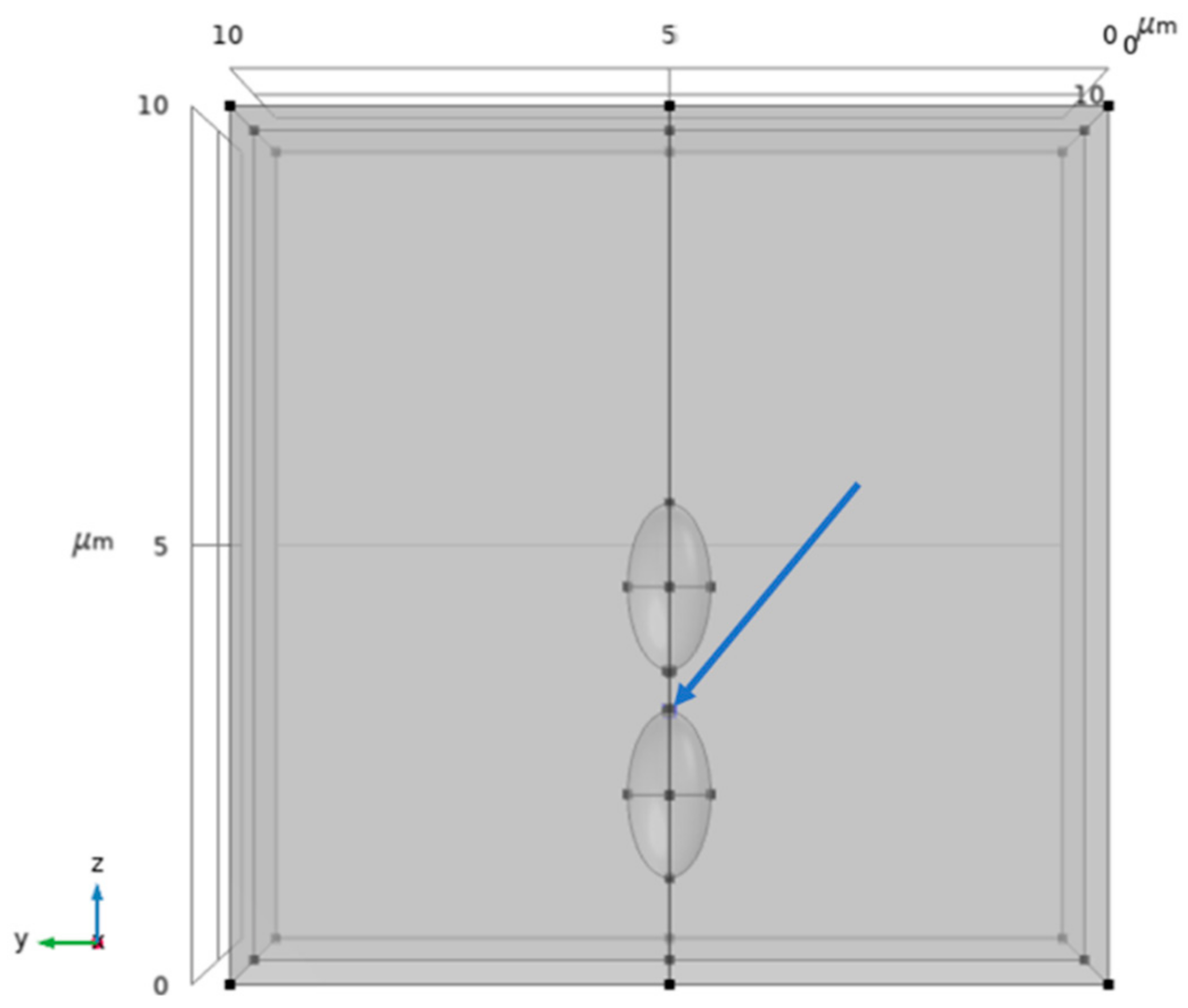
In this work, additional material features are considered for modelling XLPE’s behavior—namely, thermal expansion and hardening. Assuming the same stationary conditions as in [3,8], this work intends to further understand the evolution of voids in the XLPE insulation layer of power cables, studying the effects of geometric parameters and the intensity of the electric field on the material yield. For the sake of a safe design for the cables, the onset of XLPE yielding is here hypothesized as the onset of void coalescence, leading to the evolution of water treeing (not considered in this study). The role of relative dimensions, distance, and the shape of two interacting voids are simulated to better understand:

-

The stress and strain fields around a spherical void function of the electric field intensity;

-

How the distance between two distinct ellipsoidal voids affects the local electric field distribution and the yielding process;

-

The influence of the void volume ratio on the intensification of electric field and yielding.

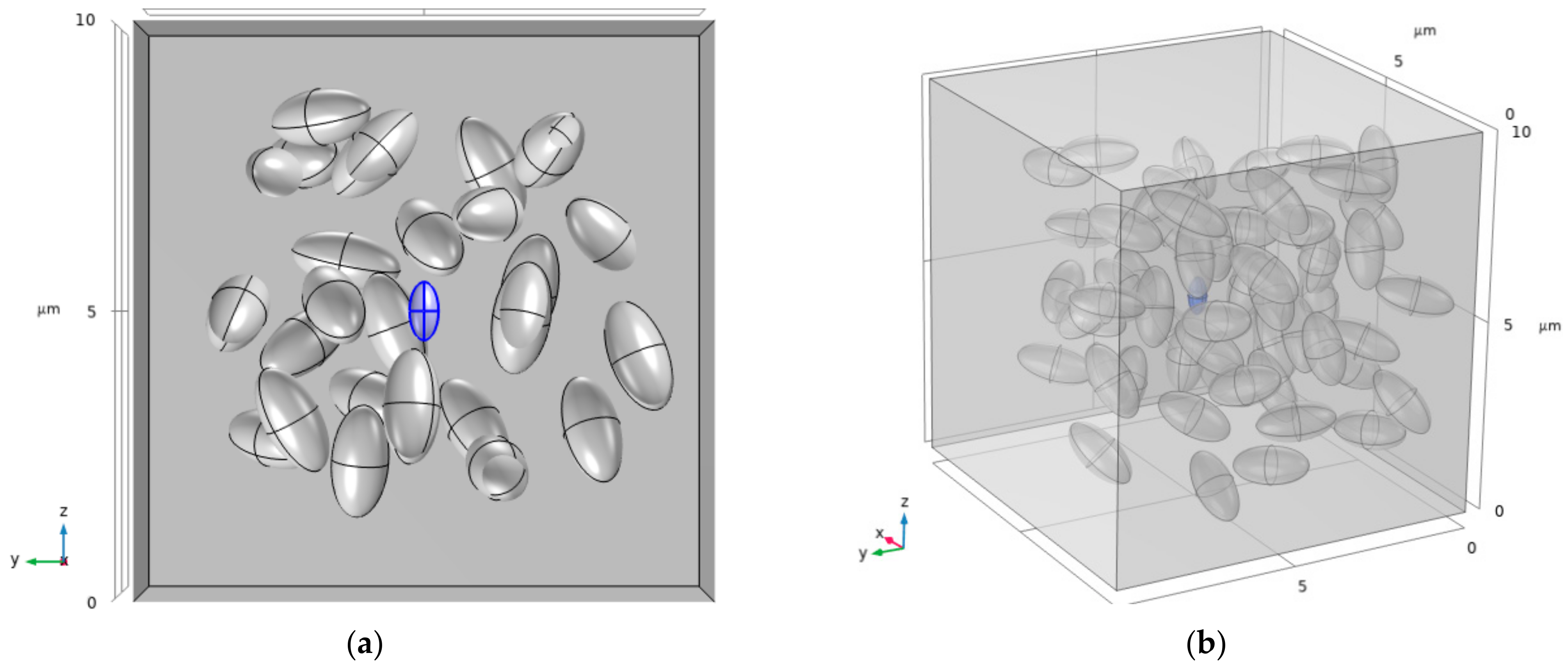
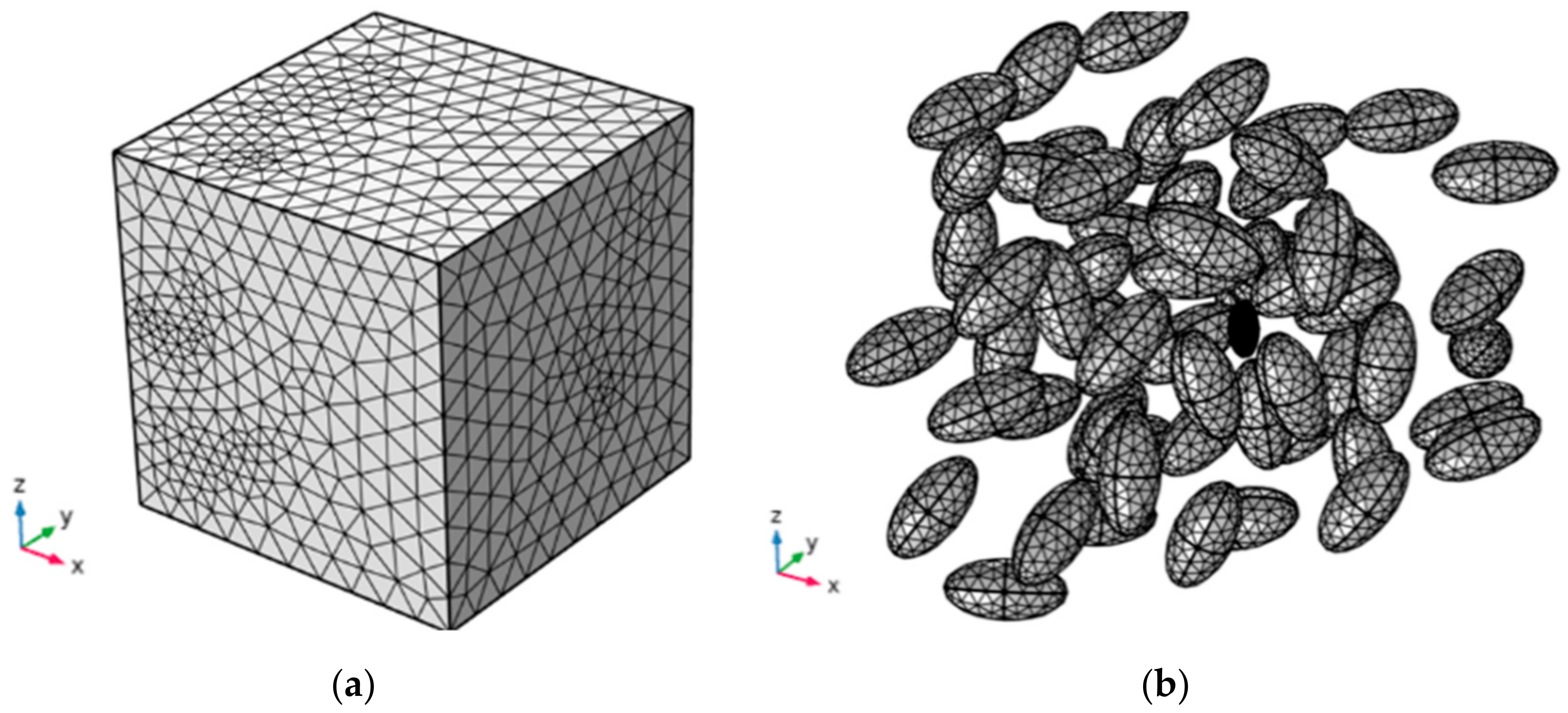
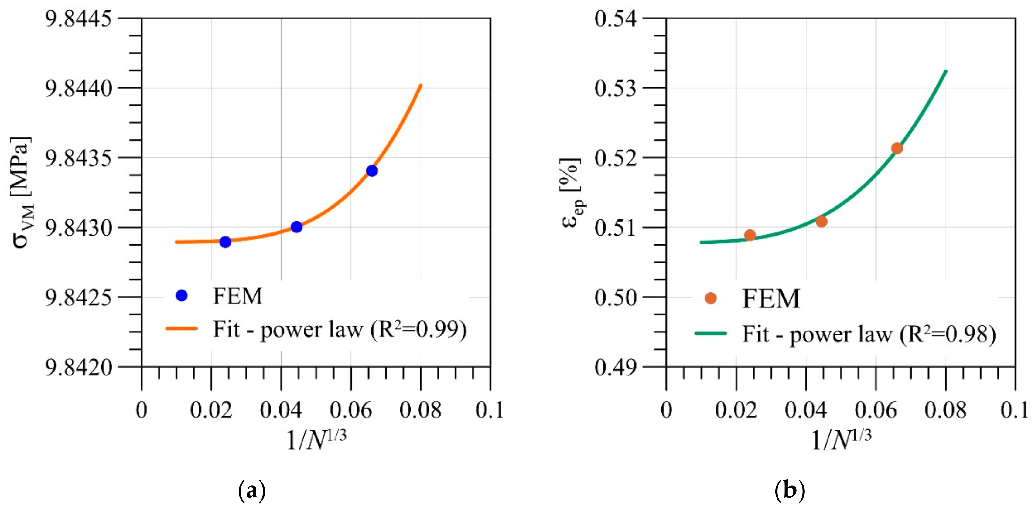
The final aim of this work is to examine the stress and strain distribution in a random distribution of N voids and to confirm the prediction by the RVE.

2. Finite Element Model Features

2.1. Brief Background on the Electromechanics Problem

A coupled electrical and mechanical 3D problem must be solved to describe water treeing inside XLPE. To this end, the “electromechanics module” of COMSOL Multiphysics has been adopted; this includes the “Structural mechanics”, “Electrostatics”, and “Moving mesh” features. Structural mechanics predicts the strain ε and stress σ field inside the model domain, in the reference configuration X. In contrast, Electrostatics gives the voltage V and the electric field E, varying with the spatial coordinate x (position in the current configuration). The coupling between the two is provided by the definition of the Maxwell stress tensor (σ^EM)—the stress generated in a dielectric immersed in an electromagnetic field. For electrostatics, the field is given by Equation (1), where 𝜖₀ is the dielectric permittivity.

$${\mathit{\sigma }}^{EM}={ϵ}_0 \mathit{E}\otimes \mathit{E}-1/2 \left({ϵ}_0 \mathit{E}\cdot \mathit{E}\right)\mathit{I}$$

(1)

The moving mesh feature is needed to deform the spatial mesh frame inside the water domain, according to the displacement of the void boundaries, governed by structural mechanics.

Before entering into the details of the finite element model, it is worth defining the types of coordinate systems used in continuum mechanics. A material particle is identified by a material (Lagrangian) coordinate 𝑿, i.e., its position in the initial reference configuration and a spatial (Eulerian) coordinate 𝒙, which describes the position in the current configuration at time t. As forces are applied to the material coordinates of the particles, which remain constant (the coordinates identify univocally the particle), the spatial coordinate changes in time. The difference between the spatial and material coordinates represents the displacement vector:

𝒖 = 𝒙 − 𝑿 = (𝑢, 𝑣, 𝑤)

(2)

In the structural mechanics module, the independent variable is the displacement field, while the material description is Lagrangian. On the other hand, the electrostatics physics are characterized by a Eulerian description and by the electric potential V as an unknown. The mechanical and dielectric properties of XLPE and water are attributed according to the material coordinates. Evidently, electrostatic properties depend on 𝒖. Due to this, a Moving Mesh physics must be used in water domains; this functionality deforms the spatial frame mesh according to the material mesh and simulates how fluid reacts to the displacement of the solid boundary, adding or removing liquid inside the domain itself (neglecting any effects of depression/compression given by the liquid on the solid–fluid interface).

All the simulations discussed in this paper are “stationary”: the electric field is static. The alternating nature of the AC current flowing in the copper wires is not considered in the current work and may be shown as future research guidelines.

2.2. Solid Models

The four case studies considered in this work are listed in

Table 1. Summary of the case studies and motivations.

Case Study ID	Motivation
1	Single void for assessing electric field levels
2	Effect of distance between two voids
3	Effect of the volume ratio of two voids
4	Random distribution of voids

. For each simulation, the representative unit element (RVE) is a cube with side l = 10 μm. Case study 1 examines, preliminarily, a single spherical void centered in the RVE (see

Table 2. Geometric parameters of case study 1 (see Figure 1).

Radius r [μm]	Spherical Void Centre Coordinates [μm]
1	(5, 5, 5)

, and Figure 1). In case studies 2 and 3, the influence of distance (see

Table 3. Geometric parameters of case study 2: ellipsoid 1 (see Figure 2).

a, b [μm]	c [μm]	P Coordinates [μm]
0.8	1.6	(5, 5, 2.5)

and

Table 4. Geometric parameters of case study 2: ellipsoid 2 (see Figure 2).

Simulation ID	a, b [μm]	c [μm]	dz [μm]	P Coordinates [μm]
2.a	0.8	1.6	0.3	(5, 5, 6)
2.b	0.8	1.6	0.7	(5, 5, 6.4)
2.c	0.8	1.6	1.3	(5, 5, 7)
2.d	0.8	1.6	1.8	(5, 5, 7.5)

and Figure 2) and volume ratio (see

Table 5. Geometric parameters of case study 3: ellipsoid 1 (see Figure 3).

a0 [μm]	b0 [μm]	c0 [μm]	P Coordinates (x0, y0, z0) [μm]
0.5	0.5	0.5	(5, 5, 2)

and

Table 6. Geometric parameters of case study 3: ellipsoid 2 (see Figure 3).

Simulation ID	Volume Ratio ϕ	a [μm]	b [μm]	c [μm]	P Coordinates [μm]
3.a	1	a0	b0	c0	(x0, y0, 3.5)
3.b	3	$\sqrt[3]{3}{a}_0$	$\sqrt[3]{3}{b}_0$	$\sqrt[3]{3}{c}_0$	(x0, y0, 3.72)
3.c	8	2a0	2b0	2c0	(x0, y0, 4)
3.d	16	$\sqrt[3]{16}{a}_0$	$\sqrt[3]{16}{b}_0$	$\sqrt[3]{16}{c}_0$	(x0, y0, 4.26)
3.e	30	$\sqrt[3]{30}{a}_0$	$\sqrt[3]{30}{b}_0$	$\sqrt[3]{30}{c}_0$	(x0, y0, 4.55)

and Figure 3) on the yielding onset of 2 aligned ellipsoidal water-filled voids, parallel to the electric field direction, is investigated.

Finally, case study 4 considers a representative volume element with a randomly distributed set of voids. It is one of the main advancements of this work, which puts the model closer to a “real” case. The geometry is obtained by using a random distribution of ellipsoids implemented in a MATLAB subroutine; this can be defined given the minimum distance between voids and the number of inclusions in the RVE (see

Table 7. Geometric parameters of case study 4: smaller central void (see Figure 4).

a [μm]	b [μm]	c [μm]	Center Coordinates [μm]
0.25	0.25	0.5	(5, 5, 5)

and

Table 8. Geometric parameters of case study 4: random distribution of ellipsoids (see Figure 4).

a [μm]	b [μm]	c [μm]	Number of Voids	Minimum Distance [μm]
0.5	0.5	1	56	0.2

and Figure 4). A smaller central void aligned along axis z is also included.

2.3. Mesh Features

Hereafter, some features of the finite element meshes adopted for the four models are detailed. A second order serendipity formulation was selected for the solid mechanics, while quadratic elements were used for the electrostatics. No reduced integration is adopted.

The RVE of Case study 1 was built with 105,000 tetrahedral elements, with a finer distribution close to the polymer–water discontinuity (Figure 5). Simulations of case study 2 and 3 were performed making use of about 220,000 tetrahedron elements. A semi-spherical partition Ω_c (r = 0.03 c) was created at the ellipsoid tips for controlling the mesh density, where electric field and stress intensification was expected (see Figure 6 and Figure 7). The proper element density and the maximum element size h_c was evaluated based on a preliminary refinement study (see mesh sensitivity analysis in Section 3). For case study 4, 200,000 tetrahedral elements were adopted (Figure 8).

2.4. Material Constitutive Model

XLPE’s mechanical properties are dependent on temperature—especially Young’s modulus (E) and the initial yield strength (σy0). In this work, as a simplifying assumption, the temperature field was assumed to be constant in space and time at 70 °C [9], neglecting any dynamic effect given by electromagnetic heating and mechanical losses. The temperature, set at 70 °C, was chosen to represent worse working conditions. XPLE visco-elastic effects were not considered. In

Table 9. Mechanical properties for XLPE [10].

E	195.6 MPa	Elastic modulus
ν	0.3	Poisson coefficient
σy0	9.82 MPa	Yield stress

,

Table 10. Thermo-electric properties of XLPE [8].

εr	2.3	Dielectric constant
α	$150\cdot {10}^{-6}{ \mathrm{K}}^{-1}$	Thermal expansion coefficient

and

Table 11. Dielectric properties of water [8].

εr

80

Dielectric constant

the adopted properties of XLPE and water are listed. Note that this temperature has some influence on the plastic deformability of XPLE, which promotes the onset of water treeing.

Tensile tests of wire-grade XLPE—detailed in [11]—carried out at room temperature were considered to extrapolate the hardening stress–strain curve (Figure 9) adopted for the numerical models. The hardening function σ_h was set as:

$${\sigma }_h\left({\epsilon }_{ep}\right)={\sigma }_p{}_{ }\left({\epsilon }_{el}+{\epsilon }_{ep}\right)-{\sigma }_{y0}$$

(3)

where ε_el is the elastic strain, ε_ep is the effective plastic strain, and σ_p is the stress estimated in [11].

2.5. Boundary Conditions

Symmetric boundary conditions have been enforced on the external surface of the representative volume element, imposing null displacement in the direction normal to the surface u_n = 0. The interface between polymer and water-filled voids is left load-free, neglecting the presence of any pressure exerted by the fluid on the void walls (see Figure 10).

The electric field is simulated inside the volume by applying a difference in potential at 2 opposed faces of the cube. The face z = 0 is grounded (V = 0), while on the opposite one—z = 10 μm—is applied a voltage V = 10 E_appl μm, where E_appl represents the average external electric field applied in the insulation as result of the AC current flowing in the wires. The normal component of the electric displacement field is set D_n = 0 on the lateral faces of the cube to ensure continuity of the electric field and no accumulation of charge on the latter (Figure 11).

“Moving Mesh” physics were applied to the water domains; the “deforming domain” feature was used to coherently deform the mesh according to the mechanical displacement of the polymer–water interfaces.

Finally, the “thermal expansion” feature was added under the “linear elastic material” behavior. The reference temperature selected was 20 °C, while the current temperature was 70 °C.

3. Results and Discussion

Some preliminary analyses are presented first; they were dedicated to the mesh sensitivity of the numerical modelling, assuming case study 3.c (see Table 6) with E_appl = 180 kV/mm. The maximum element size h_max inside the control region (defined in Section 2.3) was progressively decreased; then, σ_VM (Von Mises stress) and ε_ep (equivalent plastic strain) at one of the ellipsoid tips, shown in Figure 12, were compared. The values of h_max were 0.008 c, 0.005 c, and 0.003 c (where the semi-axis length c = 1 μm). The results are depicted in Figure 13, as a function of $1/\sqrt[3]{N}$, where N is the element number inside the control region Ω_c (Figure 6).

Hereinafter, h_max = 0.003 c was selected as the mesh density in the control volume Ω_c, representing a good compromise between computational costs and the accuracy of the solution. Assuming the theoretical extrapolated effective plastic strain ε_ep for h→0 in Figure 13b, an error can be estimated of the order of $\approx \frac{0.50902-0.5078}{0.5078}\ast 100=0.2\%$.

3.1. Single Void for Assessing Electric Field Levels (Case Study 1)

The stress components at the sphere pole S of coordinates (5, 5, 6) are plotted in Figure 14. As E_appl was increased, the compressive Maxwell stress superposed onto the pre-existing thermal expansion stress components σ_x and σ_y. In this configuration, no yielding was predicted for the typical working conditions of 100–150 kV/mm. The Von Mises stress (σ_VM) decreased in the selected range of the external electric field.

3.2. Effect of Distance between Two Voids (Case Study 2)

The polarization effect (separation of charges inside the water-filled regions) caused the intensification of the electric field at the poles of the ellipsoidal pores (see Figure 15). Due to the higher Maxwell stresses, this region was the first to yield, and here the coalescence process was expected to onset (see Figure 16 and Figure 17). The electrical field required to initiate yielding E_appl,onset is plotted in Figure 18, with a power law fitting function of the form $y=a{x}^b+c$ (coefficients in

Table 12. Case study 2: power law coefficients.

a [kV/mm]	−120.7
b	−0.366
c [kV/mm]	302.2

). The curve indicates that with a typical value for the electric field in hi-voltage cables (100–120 kV/mm), the material yielded when the void distance was less than 0.5 μm, meaning they could coalesce.

3.3. Effect of the Volume Ratio of Two Voids (Case Study 3)

As in Case study 2, the higher local electric fields and the yielding onset occurred at the smaller pore tip (see Figure 19 and Figure 20). E_appl,onset was, in this case, plotted versus the volume ratio ϕ between the two ellipsoids in Figure 21. The predicted results can be fitted using a power law regression $y=a{x}^b+c$ (coefficient of determination R² = 0.999; see

Table 13. Case study 3: power law coefficients.

a [kV/mm]	−94.62
b	0.168
c [kV/mm]	269.6

). The results showed that the forces of attraction between the polarized water molecules inside the voids increased when the volume of the pore increased.

3.4. Random Distribution of Voids (Case Study 4)

Figure 22 depicts the local electric field E_local for the random distribution case study 4, for an external applied field E_appl = 130 kV/mm. It is evident that only interactions between adjacent voids, with a distance lower than 1 μm, resulted in the amplification of the electric field (stress) at the ellipsoid tips (yielding onset, Figure 22b)—confirming the prediction of the RVE with two ellipsoidal voids at E_appl = 130 kV/mm, which is in the range of the electric fields for water treeing mentioned in the literature [3].

4. Conclusions

The study aimed at modelling water treeing in the XLPE insulation layer of submerged, high-voltage composite cables. The multiphysics FEM software “COMSOL” was used to predict the electric field-induced yielding of the material, which is supposed to be the coalescence onset of water-filled voids inside XLPE microstructure. Pores were modelled in different configurations inside a representative volume element; the role of some geometrical parameters (i.e., distance and volume ratios of the voids) was assessed in polymer yielding and then in the coalescence mechanism. Finally, a more general case of a random distribution of voids inside the unit cell was simulated, in order to be closer to a real case. The single spherical void did not yield in the operating range of E_appl = 120–250 kV/mm. Ellipsoidal voids are much more prone to yielding and coalescence; with decreasing distance between the tips of two ellipsoids, yielding onset is triggered at a lower electric field level than in a cable application. Moreover, a power law relationship has been detected between the volume ratio/tip distance and the electric field for the onset of material yielding in the smaller pores. The hypothesis of a small RVE representing the entirety of the microstructure seems to be reasonable, based on the results of the randomly dispersed void configuration. Therefore, for present purposes, the predictions of the RVE with two ellipsoids could be representative of more complex geometries, closer to a real physical microstructure. The number of voids present in the RVE has been proven to have no influence on the smaller central void—especially when the pores are far from each other. Although these results seem reasonable and in accordance with experimental findings, it must be reminded that many assumptions have been made in this initial study. Further studies should be carried out in future to shed light on other aspects (e.g., the viscoelastic behavior of XPLE, temperature variation in phases, AC currents) leading to more comprehensive simulation of the voids’ coalescence in XLPE.

References

1. Balachandran, M. Aging and Degradation Studies in Crosslinked Polyethylene (XLPE). In Crosslinkable Polyethylene; Thomas, J., Thomas, S., Ahmad, Z., Eds.; Materials Horizons: From Nature to Nanomaterials; Springer: Singapore, 2021; pp. 189–210. ISBN 9789811605130. [Google Scholar]
2. Noțingher, P.V.; Stancu, C.; Pleșa, I. Failure Mechanisms in XLPE Cables. In Crosslinkable Polyethylene; Thomas, J., Thomas, S., Ahmad, Z., Eds.; Materials Horizons: From Nature to Nanomaterials; Springer: Singapore, 2021; pp. 271–347. ISBN 9789811605130. [Google Scholar]
3. Drissi-Habti, M.; Raj-Jiyoti, D.; Vijayaraghavan, S.; Fouad, E.-C. Numerical Simulation for Void Coalescence (Water Treeing) in XLPE Insulation of Submarine Composite Power Cables. Energies 2020, 13, 5472. [Google Scholar] [CrossRef]
4. Wang, Z.; Marcolongo, P.; Lemberg, J.A.; Panganiban, B.; Evans, J.W.; Ritchie, R.O.; Wright, P.K. Mechanical Fatigue as a Mechanism of Water Tree Propagation in TR-XLPE. IEEE Trans. Dielect. Electr. Insul. 2012, 19, 321–330. [Google Scholar] [CrossRef]
5. Meziani, M.; Mekhaldi, A.; Teguar, M. Impact of Presence of Water Tree and Microcavities on the Electric Field Distribution in XLPE Insulation. In Proceedings of the 2015 4th International Conference on Electrical Engineering (ICEE), Boumerdes, Algeria, 13–15 December 2015; pp. 1–5. [Google Scholar]
6. Crine, J.-P. Influence of Electro-Mechanical Stress on Electrical Properties of Dielectric Polymers. IEEE Trans. Dielect. Electr. Insul. 2005, 12, 791–800. [Google Scholar] [CrossRef]
7. Sakamoto, H.; Yahagi, K. Electrical Capacitance of Polyethylene under Application of High DC Electric Field. Jpn. J. Appl. Phys. 1980, 19, 253–262. [Google Scholar] [CrossRef]
8. Drissi-Habti, M.; Manepalli, S.; Neginhal, A.; Carvelli, V.; Bonamy, P.-J. Numerical Simulation of Aging by Water-Trees of XPLE Insulator Used in a Single Hi-Voltage Phase of Smart Composite Power Cables for Offshore Farms. Energies 2022, 15, 1844. [Google Scholar] [CrossRef]
9. Zhang, Y.; Chen, X.; Zhang, H.; Liu, J.; Zhang, C.; Jiao, J. Analysis on the Temperature Field and the Ampacity of XLPE Submarine HV Cable Based on Electro-Thermal-Flow Multiphysics Coupling Simulation. Polymers 2020, 12, 952. [Google Scholar] [CrossRef] [PubMed] [Green Version]
10. Ansys Granta EduPack. Available online: https://www.ansys.com/fr-fr/academic/learning-resources (accessed on 8 May 2023).
11. Pirnia, F. Experimental Analyses on XLPE under Tension and Compression. Master’s Thesis, Blekinge Institute of Technology, Karlskrona, Sweden, 2014. [Google Scholar]
Figure 1. Case study 1: geometry of the RVE.
Energies 16 04620 g001
Figure 2. Case study 2: (a) cross-section x = 5 μm, (b) isometric view of the RVE.
Energies 16 04620 g002
Figure 3. Case study 3: (a) cross-section x = 5 μm, (b) isometric view of the RVE.
Energies 16 04620 g003
Figure 4. Case study 4: (a) cross-section x = 10 μm, (b) isometric view of the RVE (the smaller central void is highlighted in blue).
Energies 16 04620 g004
Figure 5. Case study 1: cross section x = 5 μm of the finite element mesh.
Energies 16 04620 g005
Figure 6. Case study 2: (a) cross-section x = 5 μm and (b) magnification of the void tip of the finite element mesh.
Energies 16 04620 g006
Figure 7. Case study 3: (a) cross-section x = 5 μm and (b) magnification of the void tip of the finite element mesh (simulation 3.c).
Energies 16 04620 g007
Figure 8. Case study 4: (a) isometric view of the RVE finite element mesh and (b) details of the void’s mesh).
Energies 16 04620 g008
Figure 9. XLPE mechanical properties: (a) constitutive stress–strain curve at 20 °C, (b) variations in the elastic modulus and yield stress with temperature.
Energies 16 04620 g009
Figure 10. Boundary conditions, shown for case study 1: (a) external surface un = 0, (b) internal surface of void F = 0.
Energies 16 04620 g010
Figure 11. Boundary conditions for the electrostatics physics, shown for case study 3: highlighted faces for (a) V = 10   E a p p l   μ m , (b) V = 0, (c) D n = 0 .
Energies 16 04620 g011
Figure 12. Ellipsoid vertex, shown by the arrow, where σVM and εep are extrapolated.
Energies 16 04620 g012
Figure 13. Mesh sensitivity for case study 3.c: (a) σVM, (b) εep at one of the void tips.
Energies 16 04620 g013
Figure 14. Case study 1: (a) map of electric field (kV/mm) on cross-section x = 5 μm; (b) Von Mises stress (σVM) and stress components (σx, σy, σz) at void pole S vs. Eappl; map of σVM for (c) Eappl = 100 kV/mm and (d) Eappl = 250 kV/mm.
Energies 16 04620 g014
Figure 15. Case study 2: maximum Elocal inside ellipsoid control volume Ωc versus dz for Eappl = 100 kV/m.
Energies 16 04620 g015
Figure 16. Case study 2: map of εep at void tip for Eappl = 203 kV/mm.
Energies 16 04620 g016
Figure 17. Case study 2: max εep inside control volume Ωc vs. external electric field Eappl: (a) dz = 0.3 μm, (b) dz = 1.8 μm.
Energies 16 04620 g017
Figure 18. Case study 2: Eappl,onset vs. distance dz.
Energies 16 04620 g018
Figure 19. Case study 3: map of Elocal on cross section x = 5 μm for (a) ϕ = 1 and (b) ϕ = 30; (c) maximum Elocal at the smaller ellipsoid tip vs. ϕ for Eappl = 100 kV/mm.
Energies 16 04620 g019aEnergies 16 04620 g019b
Figure 20. Case study 3: max εep inside control volume Ωc at the smaller ellipsoid tip vs. external electric field Eappl: (a) ϕ = 3, (b) ϕ = 30.
Energies 16 04620 g020
Figure 21. Case study 3: Eappl,onset vs. volume ratio ϕ.
Energies 16 04620 g021
Figure 22. Case study 4: (a) map of Elocal on cross section y = 5 μm for Eappl = 100 kV/mm; (b) max εep at the smaller ellipsoid tip (shown by the arrow) vs. external electric field Eappl.
Energies 16 04620 g022