Article

Initial-Productivity Prediction Method of Oil Wells for Low-Permeability Reservoirs Based on PSO-ELM Algorithm

1
School of Energy Resources, China University of Geosciences (Beijing), Haidian District, Beijing 100083, China
2
Key Laboratory of Marine Reservoir Evolution and Hydrocarbon Enrichment Mechanism, Ministry of Education, Beijing 100083, China
3
Key Laboratory of Geological Evaluation and Development Engineering of Unconventional Natural Gas Energy, Beijing 100083, China
4
The Eighth Oil Production Plant, China National Petroleum Changqing Oilfield Branch, Xi’an 710018, China
*
Author to whom correspondence should be addressed.
Energies 2023, 16(11), 4489; https://doi.org/10.3390/en16114489
Submission received: 27 April 2023 / Revised: 24 May 2023 / Accepted: 31 May 2023 / Published: 2 June 2023
(This article belongs to the Special Issue Advanced Research and Techniques on Enhanced Oil Recovery Processes)

Abstract

:
Conventional numerical solutions and empirical formulae for predicting the initial productivity of oil wells in low-permeability reservoirs are limited to specific reservoirs and relatively simple scenarios. Moreover, the few influencing factors are less considered and the application model is more ideal. A productivity prediction method based on machine learning algorithms is established to improve the lack of application performance and incomplete coverage of traditional mathematical modelling for productivity prediction. A comprehensive analysis was conducted on the JY extra-low-permeability oilfield, considering its geological structure and various factors that may impact its extraction and production. The study collected 13 factors that influence the initial productivity of 181 wells. The Spearman correlation coefficient, ReliefF feature selection algorithm, and random forest selection algorithm were used in combination to rank the importance of these factors. The screening of seven main controlling factors was completed. The particle swarm optimization–extreme learning machine algorithm was adopted to construct the initial-productivity model. The primary control factors and the known initial productivity of 127 wells were used to train the model, which was then used to verify the initial productivity of the remaining 54 wells. In the particle swarm optimization–extreme learning machine (PSO-ELM) algorithm model, the root-mean-square error (RMSE) is 0.035 and the correlation factor (R2) is 0.905. Therefore, the PSO-ELM algorithm has a high accuracy and a fast computing speed in predicting the initial productivity. This approach will provide new insights into the development of initial-productivity predictions and contribute to the efficient production of low-permeability reservoirs.

1. Introduction

The initial-productivity prediction of low-permeability reservoirs is an important fundamental task in the initial stage of reservoir exploration and development. The work can provide the basis for the development dynamic analysis, well optimization strategy plan, and reserves estimation. Recently, many scholars have proposed different methods to predict initial productivity, including a mathematical model [1,2,3], numerical simulation method [4], and drill-stem testing [5,6].
The accurate prediction of well productivity plays a pivotal role in enhancing the oil recovery of reservoirs. All data-driven productivity prediction models revolve around the feature selection and forecasting model. Firstly, we consider the feature selection. There are many factors affecting the initial productivity. Most researchers studying the main controlling factors primarily focus on geological factors and dynamic development factors [7,8,9,10,11]. Wenli Ma et al. proposed the Pearson maximum information coefficient correlation synthesis analysis method to identify 13 main control factors for the initial shale gas productivity [12]. Hao Chen et al. used a combination of Pearson’s coefficient, Spearman’s coefficient, and Kendall’s coefficient methods to optimize the main control factors [13]. Rastogi et al. used the SelectKBest feature selection, tree regression, Pearson’s correlation coefficient, recursive feature elimination, and correlation feature selection algorithms to select the main control factors for the impact of hydraulic fracturing chemicals on the unconventional reservoirs’ productivity [14]. Zhao Wang et al. established the XGBoost linear regression prediction model to predict the initial productivity and evaluate the main controlling factors [15]. The above scholars used the feature factor selection algorithm, screening and ranking the influencing factors to finally determine the main controlling factors affecting productivity [16,17,18,19]. However, the majority of current studies on the main control factors solely emphasizes geological factors and dynamic development factors, overlooking the influence of the non-numerical variables in engineering factors on productivity. Previous research has primarily focused on using algorithms to analyze the correlation between input and output data, but the results often lack practical application explanations. In contrast, the author of this study utilized a combination of factor selection algorithms, reservoir engineering knowledge, and production experience to screen for the main controlling factors. This approach resulted in selected factors that are more aligned with practical applications, rather than relying solely on a single algorithm for selection.
Multiple machine learning algorithms have been applied to build productivity prediction models, such as neural networks, support vector machines, random forests, and Bayesian networks. Yintao Dong et al. constructed the XGBoost algorithm without physical constraints to reduce the relative error in achieving a highly accurate initial productivity [20]. Yapeng Tian et al. used a genetic algorithm to optimize the weights and thresholds of the neural network to improve the accuracy of predicting the initial productivity of shale gas [21]. Hao Chen et al. applied the support vector machine to predict the initial productivity of horizontal wells’ volumetric fracturing in tight reservoirs. Hui-Hai Liu used the incorporation of physics into an ML model predicting well productivity [13]. On the basis of LSTM and DNN neural networks, DongXiao Hu conducted the development of a novel fitting function–neural network synergistic dynamic productivity prediction model for shale gas wells [22]. Through an analysis of the aforementioned prediction model studies, it is evident that the majority of scholars have employed machine learning algorithms for data mining in order to predict the initial productivity of reservoirs. Additionally, they have utilized diverse optimization algorithms to enhance the accuracy of these productivity models [23,24,25,26,27]. However, the author proposes an initial-productivity prediction model that is aligned with the production in the research area. The model has been compared with various other models and has shown a high prediction accuracy, fast running speed, and strong robustness.
In summary, in order to predict the productivity of low-permeability reservoirs, a comprehensive approach combining the Spearman correlation coefficient, random forest, and ReliefF feature selection algorithms is employed. This method allows for the ranking of 13 influencing factors from three aspects of geological factors, engineering factors, and dynamic development factors. Seven main controlling factors are identified by combining the reservoir engineering theory and importance ranking. There is a complex nonlinear relationship between the seven main controlling factors and the productivity of the well. In order to better predict the initial-production capacity of oil wells, the introduction of the extreme learning machine algorithm can better deal with the nonlinear prediction regression problem. However, since the initial value of the extreme learning machine is generated randomly, the prediction accuracy will be affected. In order to reduce this error, the author uses the particle swarm optimization algorithm to optimize the input weight and threshold of the extreme learning machine. This model aims to facilitate the practical application of the initial-productivity assessment, providing valuable insights for reservoir evaluation.
In this paper, the author introduces an innovative approach by employing the PSO-ELM algorithm for predicting the initial productivity of low-permeability reservoirs. The main works of this research are as follows: Firstly, Section 2 describes the selection of characteristic factors. Secondly, Section 3 introduces the main theory of the main controlling factors’ selection. Thirdly, Section 4 states the main theory of establishing the initial-productivity prediction model. Finally, Section 5 concludes the work of the paper. This initial-productivity prediction model was implemented in the Matrix Laboratory.

2. Selection of Characteristic Factors

This study focuses on identifying the key factors that affect the initial productivity of low-permeability reservoirs. The factors are categorized into three aspects: geological factors, engineering factors, and dynamic development factors. The selection of these factors is based on the original data collected from actual oilfields. A combination of production experience and reservoir engineering knowledge is used to screen and identify the most significant factors. This study selects five geological factors, including porosity, permeability of the oil formation, initial oil saturation, coefficient of variation of stratigraphic permeability, and formation permeability grade difference, as indicators of low-permeability reservoirs. Additionally, four engineering factors are considered, including reservoir shot thickness, fracturing fluid sand content ratio, fracturing fluid discharge, and reservoir modification method. Finally, four dynamic development factors, namely, water content, production pressure difference, pumping depth and dynamic fluid surface depth, are selected for dynamic development factors.
Based on the initial-productivity data collected from 181 wells in the low-permeability oilfield, specifically focusing on the first 60 days, the aforementioned 13 characteristic factors were carefully selected and collated. This resulted in a comprehensive data set of 181 instances, which serves as a valuable foundation for conducting the initial-productivity analysis. Table 1 displays the distribution range of the base data used for the prediction model. To ensure consistency, non-numerical variables in the engineering factors were transformed using the label-encoding numbering process, resulting in corresponding numerical variables. This allowed us to obtain the values for each individual well.

3. Selection and Analysis of Main Control Factors

This study utilizes the combination feature selection algorithm to identify the main controlling factors that affect low-permeability reservoirs. Utilizing the main controlling factors and removing the irrelevant factor of productivity can avoid over-fitting and quantitative calculation. The 13 characteristic factors mentioned above are used as input layer data for the initial-productivity forecast. Finally, through the correlation between each characteristic factor and the initial productivity, the rational reasonable ranking was carried out.

3.1. Spearman’s Correlation Coefficient Method

The Spearman correlation coefficient (SCC) is used as a method of estimating the correlation between two variables [28,29,30]. The correlation between the variables is reflected through the difference of the corresponding series of two pairs of grades. The closer the Spearman correlation coefficient is to +1 or −1, the stronger the correlation is between the two variables.
The Spearman correlation coefficient is calculated as
ρ = i = 1 n x i x ¯ y i y ¯ i = 1 n x i x ¯ 2 i = 1 n y i y ¯ 2
where x i and y i are the values of the characteristic factors x and y , respectively; and n is the maximum productivity of the sample.

3.2. ReliefF Feature Selection Algorithm

The ReliefF feature selection algorithm utilizes the features of the samples for learning and training. It begins by randomly selecting one sample from the training data set D of the oil well. The distance between this sample and the other samples is used to determine the weight of the feature factor. The algorithm then continuously searches for the nearest-neighbor samples to update the weight of the feature factor [31,32,33,34]. Finally, the first few items with a higher weight of the feature are selected as the main control factor.
Consider the set of samples S = S 1 , S 2 , , S m ; each sample contains p   features, s i = s i 1 , s i 2 , , s i p , and 1 i m . The values of the features are nominal or numerical. The difference between two samples s i and s j ( l i j m ) on feature t ( 1 t p ) chosen randomly in the training set D is defined as follows:
If the features of sample R are nominal features for the label-encoding numbering process, we can obtain the numerical type. If the features of sample R are numerical, we use the formula directly for calculation. The specific formula is as follows:
d i f f t , s i , s j = 0                                 s i t = s j t 1                                 s i t s j t s i r s j r m a x t m i n t           t   i s   c o n t i n u o u s
where m a x t and m i n t are the maximum and minimum weights of the characteristic factors, respectively;
A sample s i is randomly selected from the sample set D . A sample s i is taken as the centre. Then, k near-neighbor samples nearest to s i are selected from the samples of the same kind in the sample set. k samples of near hits are found from the sample set of the same kind. The weight W A of this sample is calculated. The weight value W A of this feature is updated.
W A = W A j = 1 K d i f f t , s j , H j / m * k + C c l a s s R p c 1 p c l a s s s i j = 1 K d i f f t , s j , M j / m * k
where the number of samples sampled is m ; the number of nearest-neighbor samples is k ; H j represents the characteristics of similar samples; and M j represents the characteristics of dissimilar samples.

3.3. Random Forest Selection Algorithm

A random forest is created by combining multiple decision trees in a random manner [35,36,37,38]. The regression results of the decision trees are then used to make predictions. The algorithm determines the relative importance of the characteristic factors in predicting the target variable by calculating the out-of-bag error rate.
I X i = e r r O O B 2 i e r r O O B 1 i / N
where the i -th importance of feature X , e r r O O B 2 i is the out-of-bag data error after adding random noise. e r r O O B 1 i is the corresponding out-of-bag data error for each decision tree and is selected to calculate the out-of-bag data error.
The value of the out-of-bag data error is an indicator of the importance of a feature. If the accuracy of the out-of-bag data decreases significantly after adding random noise ( e r r O O B 2 increases significantly), this suggests that the feature has a significant impact on the prediction results of the sample, thereby indicating a relatively high level of importance.

3.4. Analysis and Determination of the Main Control Factors

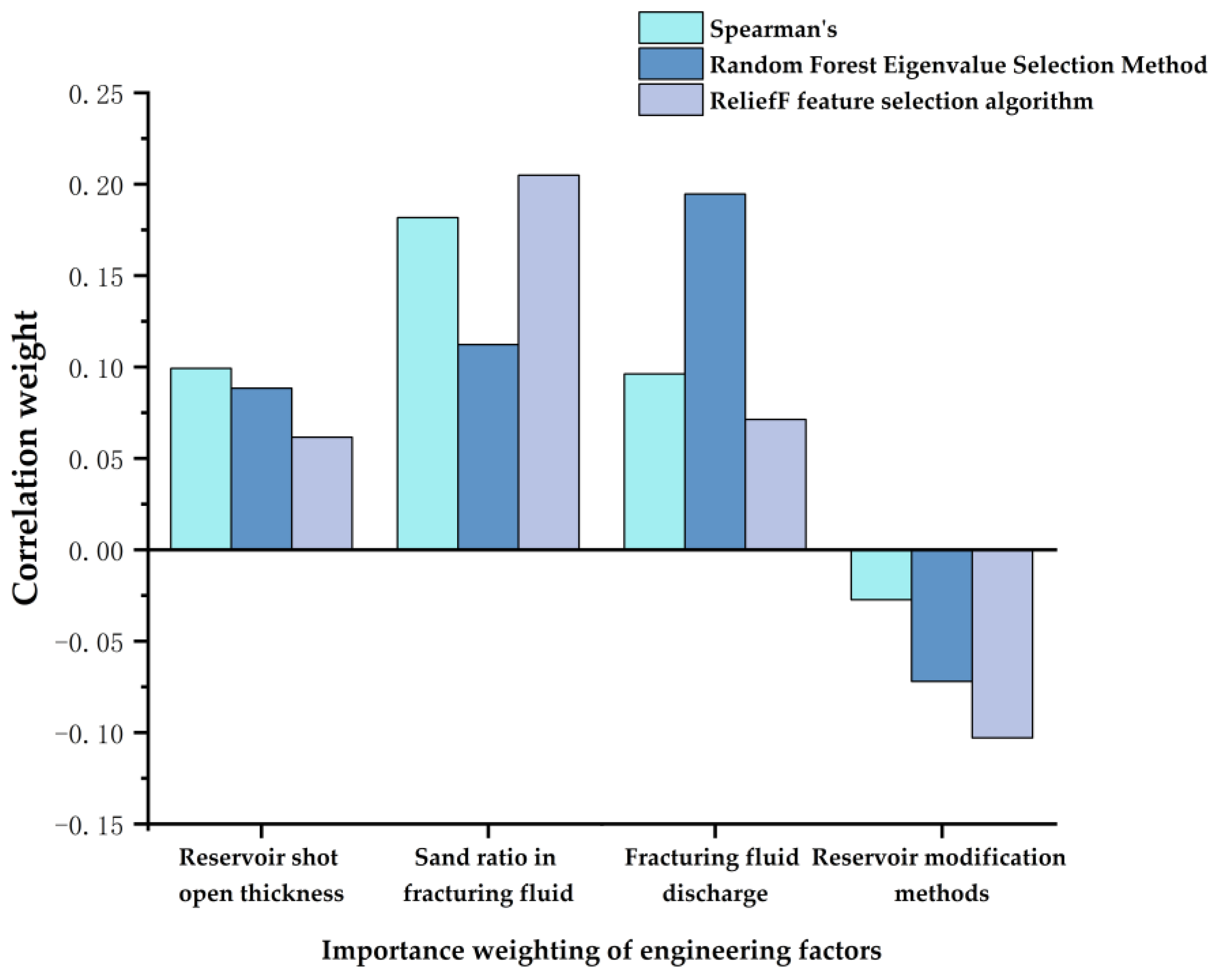
This study employed a combination of Spearman’s correlation coefficient, the ReliefF feature selection algorithm, and the random forest selection algorithm to identify the main controlling factors among thirteen feature factors, including geological factors, engineering factors, and dynamic development factors. The calculated weights were comprehensively ranked and presented in Figure 1, Figure 2 and Figure 3. The results show that seven factors were selected as the main controlling factors, as presented in Table 2.
Our study utilizes a combination feature selection algorithm to identify seven main controlling factors, as shown in Figure 1, Figure 2 and Figure 3. The RF algorithm removes factors to calculate the corresponding out-of-bag data error, which differs from the other two methods. Although there are some numerical differences in the importance rank required by the three methods, the results of their importance evaluations converge.
Through this result of the importance rank, we can analyze it to obtain the importance rank. The importance rank of geological features can be obtained as follows: porosity > permeability > stratigraphic permeability grade difference > coefficient of variation of straigraphic permeability > initial oil content saturation (from Figure 1). The ranking of engineering factors is as follows: sand ratio in fracturing fluid > fracturing fluid discharge > reservoir shot open thickness > reservoir modification methods (from Figure 2). In terms of dynamic development factors, the importance ranking is as follows: pump depth > production differential pressure > depth of dynamic fluid level > water content (from Figure 3).
The study identified seven main controlling factors. Firstly, there are geological factors such as porosity, permeability of the oil formation, and the difference in stratigraphic permeability grades. Engineering factors such as the sand ratio in fracturing fluid and fracturing fluid discharge were also found to be significant. Additionally, dynamic development factors such as production differential pressure and pump depth were identified as important considerations.

4. Initial-Productivity Forecasting Model

4.1. Fundamentals of the Extreme Learning Machine Algorithm

4.1.1. Overview of the Algorithm

The ELM algorithm is a type of single-hidden-layer feedforward neural network (SLFNS) that exhibits high operational efficiency, correctness, and strong generalization performance with few training parameters. In contrast to traditional neural networks, the algorithm randomly determines the weight vector W and threshold matrix b for the hidden layer, with only the number of neurons in the hidden layer being specified [39,40,41,42,43]. During the execution of the algorithm, there is no need to adjust the values of W and b. The predicted target value can be approximated by the excitation function g x , which is infinitely differentiable for any interval. Figure 4 shows the network structure of the ELM model.

4.1.2. Mathematical Models

The input matrix X corresponds to the n neurons in the input layer of the ELM algorithm, which is X = x i 1 , x i 2 , , x i n   T ϵ R n . The output matrix corresponds to the m neurons in the output layer, which is T = t i 1 , t i 2 , , t i m   T ϵ R m . There are l   neurons in the hidden layer. The activation function g x is modeled as
i = 1 l β i g w i x j + b i = O j j = 1 , 2 , , n
where W i = W i 1 , W i 2 , , W i n T is the input node and the input weight of the i -th hidden-layer neuron node. β i = β i 1 , β i 2 , , β i m T is the output node with the output weight of the i -th neuron node.
H is the output matrix of the ELM hidden layer, and can be expressed as
H = g w 1 x 1 + b 1 g w 1 x 2 + b 1 g w 1 x n + b 1 g w 2 x 1 + b 2 g w l x 1 + b l g w 2 x 2 + b 2 g w l x 2 + b l   g w 2 x n + b 2   g w l x 1 + b l
This is expressed as H β = T , where T is the transpose of the matrix T .
The target output of a single-hidden-layer neural network learning is zero error. It is infinitely close to the test sample and can be expressed as
j = 1 N | | o j t j | | = 0
We are training a single-hidden-layer neural network with a large number of sample data. When the activation function g x is infinitely differentiable, the W i , b i of the input layer to the hidden layer is determined. The error model for ELM can be obtained as
ε = m i n | | H β T | |
where ε is the error value of the ELM algorithm.
When the error is less than the preset error value, the output weight value β can be calculated as H * T . According to the least squares criterion, H * is the generalized inverse matrix of the output of the hidden layer.

4.2. Fundamentals of the Particle Swarm Optimization–Extreme Learning Machine Algorithm

4.2.1. Overview of the Algorithm

The particle swarm optimization algorithm simulates the foraging behavior of a flock of birds, where individuals within the group share and exchange information to continuously iterate and search for the optimal particle. This search process involves two attributes: the particle’s velocity and position [44,45].

4.2.2. Mathematical Models for Particle Swarm Optimization Algorithms

Suppose there are n particles in D-dimensional space; the i -th particle ( 1 i n ) and its position can be represented as X i = [ X i 1 ,   X i 2 , , X i D ]T. Its velocity is represented as V i = [ V i 1 , V i 2 , , V i D ]T. The root-mean-square error (RMSE) is a measure of the deviation between the initial-productivity prediction and the actual tested initial productivity. It is used as the fitness function to calculate the fitness value of each particle. A smaller RMSE value indicates a smaller deviation of the initial-productivity prediction model and higher prediction accuracy. Therefore, the particle with the smallest RMSE value is considered the best. The current best value of the i -th particle, the individual extreme value, can be expressed as P b e s t i = [ P b e s t i 1 , P b e s t i 2 , , P b e s t i D ]T. The current best value of the population, the global extreme value, can be expressed as G b e s t i = [ G b e s t i 1 , G b e s t i 2 , , G b e s t i D ]T.
ELM training outputs the root-mean-square error (RMSE) as the fitness value of PSO.
F i t n e s s = 1 N i = 1 n y r e a l y i 2
where y r e a l and y i are the output value of the desired sample and the actual predicted value of the model.
When the adaptation values of PSO are continuously calculated, the two extreme values P b e s t i and G b e s t i are searched. Its velocity and position are continuously updated through Equations (10) and (11), as follows:
V i k + 1 = ω i · V i k + c 1 · r 1 P b e s t i k X i k + c 2 · r 2 G b e s t i k X i k
X i k + 1 = X i k + V i k + 1
where V i k ,   X i k are the velocity and position of the k time and i -th particle.
P b e s t i k ,   G b e s t i k are the individual extremes and global extremes of the k time and i -th particle.
w i represents the weight values for balancing the individual-extreme-value finding ability and the global finding ability;
C 1 , C 2 are learning factors. They reflect the importance of individual extreme values and global extreme values.
r 1 , r 2 are random numbers within 0 to 1.
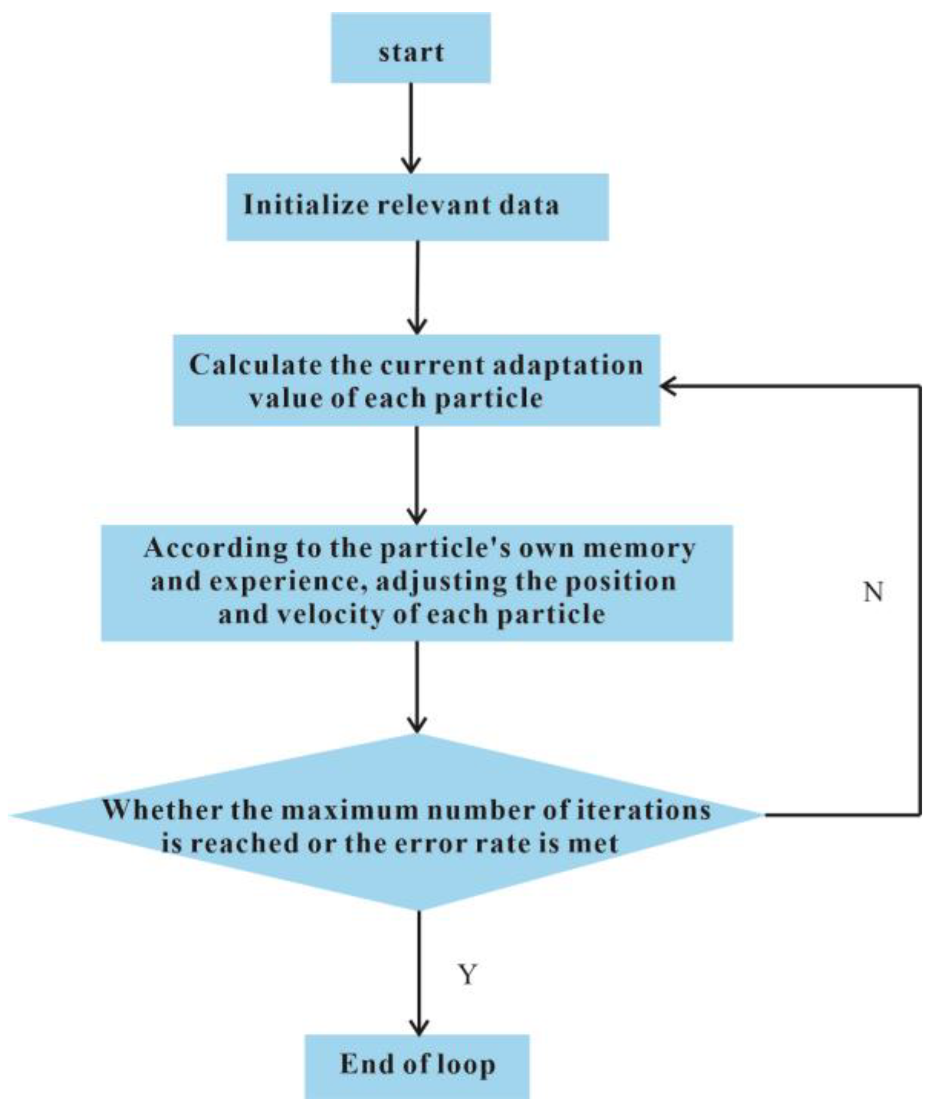
The basic flow of the particle swarm algorithm is as follows:
In the first step, the initial parameters are setting, which include the population size, dimensionality, initial speed, and position of each particle, as well as the number of iterations and the error rate size.
In the second step, the function has been set up with a constant or extreme value problem, and the current fitness value of each particle has been determined.
In the third step, each particle’s position and velocity are adjusted based on its own memory and experience.
In the fourth step, the termination condition is set to find the optimal value. The algorithm ends when the number of iterations reaches the maximum. If there is no optimal result, the algorithm continues to be executed from the second step.
The whole process is represented in Figure 5.

4.3. Particle Swarm Optimization–Extreme Learning Machine Algorithm

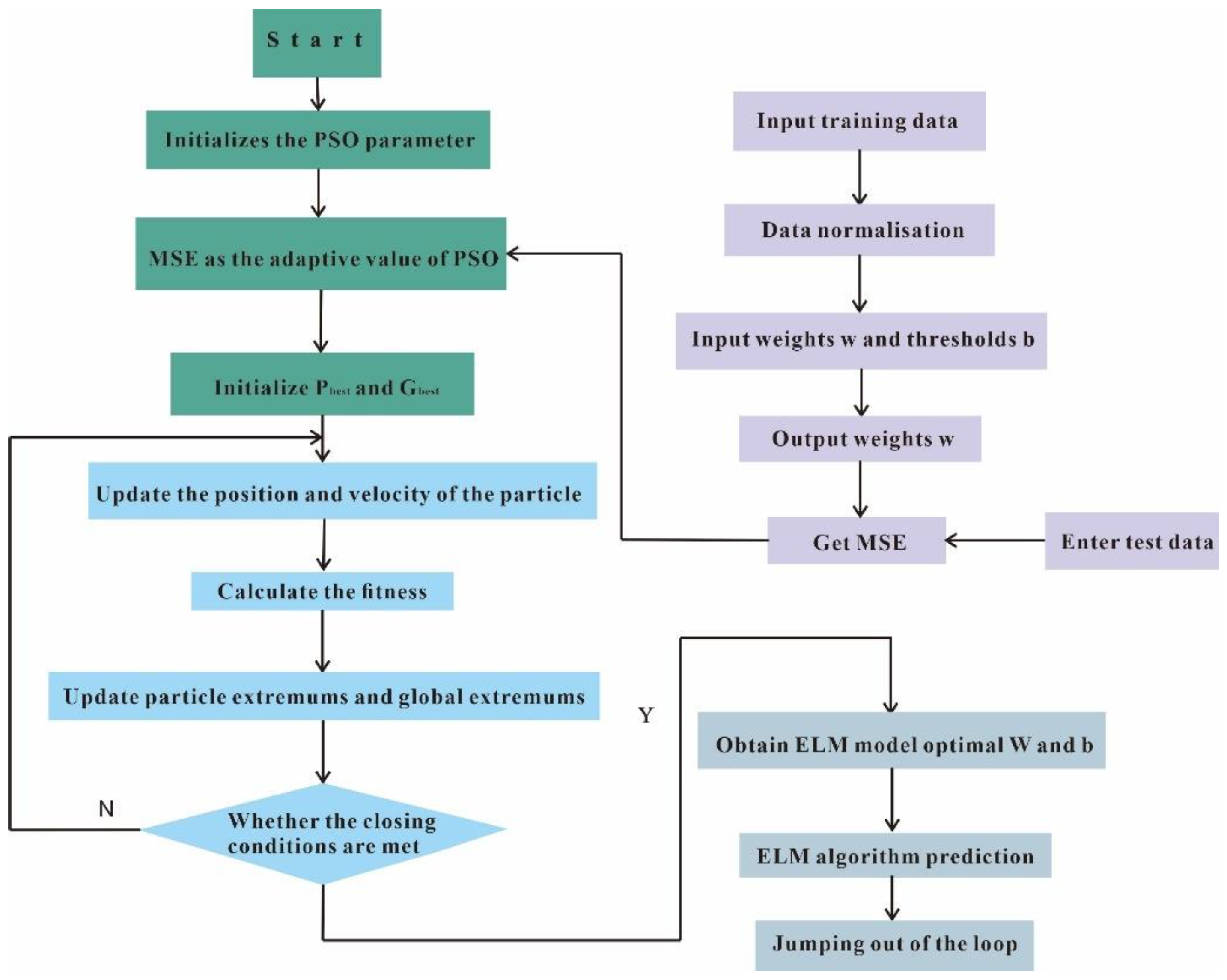
In the ELM algorithm, the initial weights ( w ) and layer bias ( b ) are randomly generated. To find the optimal values for W and b, the particle swarm optimization (PSO) algorithm is employed. The PSO algorithm continuously adjusts the parameter values to reduce the mean squared error (MSE) value. This approach results in the construction of an optimum PSO-ELM initial-productivity prediction model [46].
The PSO-ELM initial-productivity prediction model is used in this paper. The specific PSO-ELM algorithm process is shown as follows:
Firstly, the input layers consist of data on the main control factors that affect the initial productivity of the low-permeability reservoir. The data are then divided into training and detection data, and pre-processed accordingly;
Secondly, to set up the relevant parameters of the particle swarm initializing the input weight W and the implied layer threshold b of the ELM algorithm, we can use a trial-and-error approach or a more systematic method such as grid search. The value of w and b will depend on the specific problem and data set being used, so it is important to experiment with different values to find the optimal combination that yields the best performance;
Thirdly, the mean squared error MSE is calculated by using the predicted values and the actual test-data values. It takes the MSE as the fitness value for PSO;
Fourthly, the particle swarm optimization algorithm involves continuously updating the positions and velocities of particles to obtain their optimal fitness values. By calculating the fitness values of each particle, we can determine the optimal input weights W and the layer threshold b, while ensuring that the mean squared error (MSE) remains within the allowed range;
Fifthly, the optimal W and b are substituted into the ELM algorithm for prediction to achieve accurate prediction for the model.
The flow of THE PSO-ELM algorithm is shown in Figure 6.

5. Example Applications

5.1. Research Area

The proposed PSO-ELM algorithm model is utilized to predict the initial productivity of wells in the JY oilfield. This oilfield is situated in the western part of the middle region of the northern Shaanxi slope in the Ordos Basin. The Chang 8 reservoir of the Triassic Yanchang Formation is the primary oil-bearing formation in this area. The porosity of the formation ranges from 8 % to 25 % with an average of 11.3 % , while the permeability ranges from 0.01 to 20   mD with an average value of 0.64   mD . The research area pertains to a reservoir that is typical of the low-porosity and low-permeability type. The current initial development of the reservoir is characterized by the low productivity of individual wells, early emergence of water, insufficient formation energy, and rapid decline in well productivity.

5.2. Construction of the Initial-Productivity Model and Evaluation Analysis

This study utilized the PSO-ELM algorithm to construct a model for predicting initial productivity. The model was trained using data from 127 wells in the JY low-permeability field and seven main control factors. To verify the accuracy of the model, the initial productivity of 54 wells was simulated.
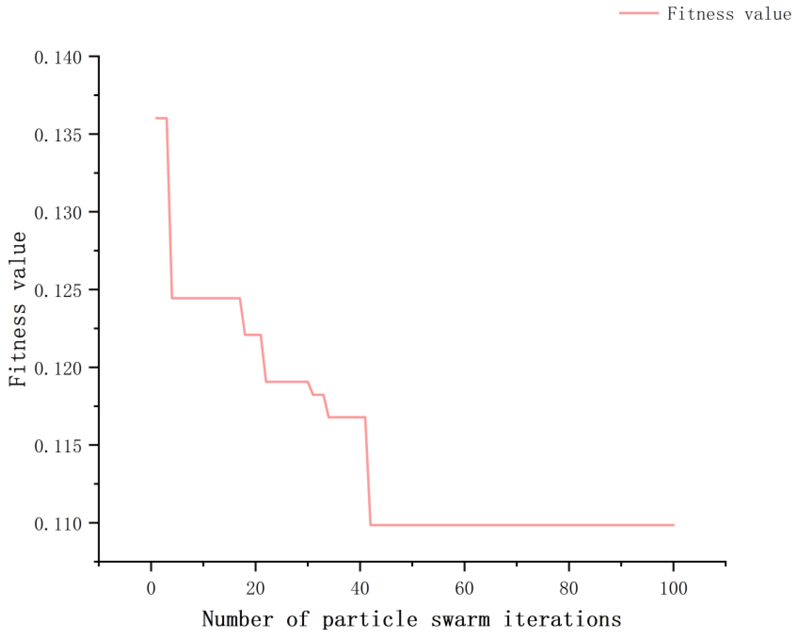
In the optimization process of the PSO algorithm, the initial parameters are set as follows: learning factor c 1 = 1.45 , c 2 = 1.64 ; and the minimum value of inertia factor w m i n = 0.1 , and the maximum value w m a x = 0.8 . The population size is 30. The maximum number of iterations is 100 and the error threshold is 10 6 . The iteration times of PSO optimization reached the 42nd time and the adaptive value tended to be stable. The curve of PSO optimization was shown in Figure 7.
In the construction process of the ELM algorithm model, the number of hidden layers is set at 8. The optimized W and b are, respectively:
W = 0.0143 0.0002 0.0168 0.1862 0.2715 0.0651 0.0135 0.3440 0.0972 0.0525 0.1683 0.0038   0.0586 0.0293 0.1531     0.0778 0.0853 0.1892 0.0144 0.0122 0.0529 0.0183 0.0726 0.0128 0.0376 0.1785 0.0274 0.0230 0.02694 0.0039 0.0306 0.3393 0.0186 0.0021 0.0273 0.0220 0.0461 0.2216 0.0211 0.0341 0.0276 0.0280 0.0188 0.0080 0.0361 0.0211 0.0141 0.0459 0.0075 0.0990 0.0272 0.0111 0.2207 0.0214 0.1389 0.0007   and b = 0.0089 ,   0.2436 , 0.0215 ,   0.1257 ,   0.0866 ,   0.0324 ,   0.0015 ,   0.0940 T .
A PSO-ELM model was constructed using 127 groups of training data. The model’s evaluation effect showed that the RMSE is 0.0145, MAE is 0.854, and R2 is 0.911. The model’s learning effect is very close to the training set data, making it a reliable tool for prediction.
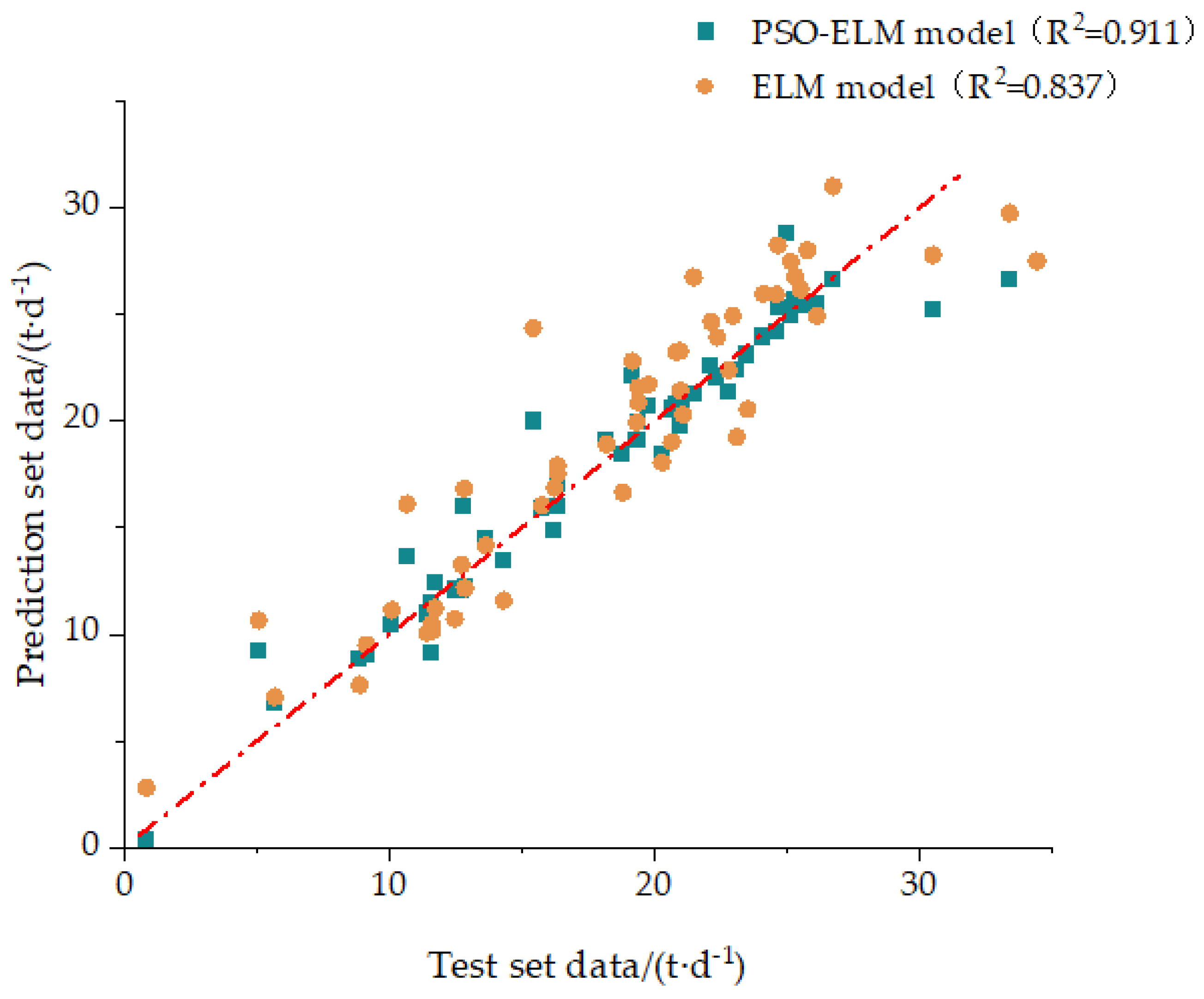
Two prediction models, namely, PSO-ELM and ELM, were constructed using the test-set data and prediction-set data to estimate initial productivity. The predicted values of both models were compared with the actual values and shown in Figure 8.
Obviously, as shown in Figure 8, the initial productivity predicted by PSO-ELM is closer to the zero-error line than that predicted by the ELM model. The ELM algorithm models w and b are optimized by using particle swarm optimization, which makes the value predicted by the PSO-ELM algorithm closer to the actual value. That is to say, the algorithm has a higher accuracy. The PSO-ELM algorithm error is made smaller and its running time is more than five seconds shorter than the unoptimized ELM model, whereas, when the predicted initial-productivity value of the two models is greater than 30, the forecast deviates from the actual value and the predicted value is lower than the actual value, and when the predicted initial-productivity value is 15, the predicted value is higher than the actual value. This is because, in the two models, the two main controlling factors, fracturing fluid displacement and production pressure difference, have a greater influence on the prediction weight. At the same time, the optimized ELM model has better adaptability. Because w and b are constantly adjusted, the model is more consistent with the predicted value.

5.3. Comparison of Different Forecasting Models

We select three commonly used performance measures: root-mean-square error (RMSE), mean absolute error (MAE), and coefficient of determination (R2). They are selected to evaluate the forecasting performance of the models. Their evaluation of the initial-productivity forecasting results is calculated as follows:
R M S E = 1 n i = 1 n y i y ^ i 2
M A E = 1 n i = 1 n y i y ^ i
R 2 = i = 1 n y ^ i y ¯ i 2 i = 1 n y i y ¯ i 2
where y i is the actual initial productivity of the i -th well; y ^ i is the predicted initial productivity of the i -th well; and y ¯ i is the average of the initial productivity. The closer the values of RMSE and MAE are to 0, the closer the value of R 2 is to 1, and the better the prediction results will perform.
To evaluate the effectiveness of the PSO-ELM algorithm, this study employs three prediction models: random forest (RF), back propagation neural network (BP), and recurrent neural network (RNN). The initial productivity of these models is compared using cross-sectional data from 54 wells. Figure 9 illustrates the comparison of the predicted and test-set data for each model.
In Figure 9, it is evident that the overall predicted value of the four prediction models is low when the model predicts the actual value to be greater than 30. The PSO-ELM, RNN, and BP models show small prediction errors, while the RF model shows a large prediction error. This is because the RF model is determined by multiple random decision trees voting, which gives it a good tolerance for noisy data but reduces the accuracy of predicting individual data. When the predicted actual value is high, the two main controlling factors are fracturing fluid displacement and production pressure difference in the input layer, which have a larger influence on the predicted value. However, the actual data of these two main controlling factors are not particularly large in the same class, resulting in some errors between the predicted and actual values.
When the value of the model predicting the productivity is less than seven, all four prediction models output a value that is too high. The RF model has the largest prediction error among the four models, which aligns with the analysis results mentioned above. However, when considering the weight of the predicted value influenced by the main controlling factors in the input layer of the model, the sand content ratio and porosity weight of the fracturing fluid have the greatest impact. The two main control factor data values in this set of data are too large in the same category, resulting in a large prediction. To sum up, there are two reasons for the analysis of the above points with large errors: (1) The model requires more in-depth learning on data pertaining to special points in order to accurately predict them. Unfortunately, the training set used in this paper only contains a very small amount of such data. (2) To improve the accuracy of the model, it is necessary to consider more engineering factors. The current model in this paper is based on only seven main control factors, which is insufficient for achieving a high-accuracy prediction for the entire range of data.
In summary, in view of the two situations, there are some errors in the prediction results of the four different models. However, the error of the PSO-ELM model is smaller. This shows that the model has good robustness and adaptability.
The test-data evaluation results of each of their models are shown in Table 3.
Obviously, the PSO-ELM algorithm has the smallest error (RMSE and MAE) and the highest accuracy (R2) in the model. Moreover, its running speed is faster. As the amount of sample data increases, the advantage of its model running speed becomes more and more obvious. This suggests that the PSO-ELM algorithm can handle the high-complexity characteristics of initial-productivity forecasting more effectively than RF, BP, and RNN. It is more suitable as a forecasting method for the dynamic analysis of oilfield initial productivity.

6. Discussion

The prediction model has good application in the petroleum industry. It also has a wide range of applications in the other industry, including initial-production capacity and peak prediction of natural gas production [47], as well as predicting the head of aquifers [48,49], carbon emissions [50,51], electricity, electric power, and electric load [52,53]. This data-driven forecasting model has a significant impact on the industry’s forecasting research.
In this paper, based on the advantage of the ELM algorithm where it runs quickly due to its single hidden layer, the PSO-ELM model was developed by integrating PSO optimization techniques. It improves the accuracy of the whole prediction model. Although other controlled algorithms are limited in this paper, we can observe that the advantages of this prediction model are more prominent in the evaluation results. It is consistent with the results of the initial predictivity of the JY oilfield.
The model currently performs well on other wells in the JY oilfield. However, it has not been applied to other oilfields with different geological factors, engineering factors, and dynamic development factors. There may be a possibility that the accuracy of the prediction model’s prediction would be reduced in other fields. The replacement of the input data source may make the parameters of the prediction model unsuitable for the new prediction model. It is necessary to adjust the parameters of the prediction model to meet the initial-productivity prediction of the oilfield.

7. Conclusions

This study has shown that the prediction of initial productivity is extremely important for the development process of low-permeability oilfields. The accuracy and precision of the model have been verified by the test data. Therefore, the initial-productivity forecasting model can guide the fundamental task in the initial stage of reservoir exploration and development.
The machine learning model solves the problems of poor adaptability and the lower consideration of influencing factors in traditional mathematical models.
(1)
This paper proposes a combination feature selection algorithm that utilizes the correlation between characteristic factors and initial productivity to provide a reasonable importance rank. The resulting main controlling factors are better suited for engineering applications in the research area.
(2)
Combination feature selection algorithms select seven main controlling factors. Moreover, the seven main controlling factors are porosity, permeability of the oil formation, the stratigraphic permeability grade difference, sand ratio in fracturing fluid, fracturing fluid discharge, production differential pressure, and pump depth.
(3)
The PSO-ELM model achieves a higher accuracy and faster speed to predict the productivity of oil wells. The model’s error evaluation indicates promising results, with an RMSE of 0.0345, MAE of 1.008, and an R2 value of 0.905. This evaluation index is better than other models.
(4)
This data-driven prediction model can also be applied to the other reservoirs with similar physical properties and geological characteristics. It can be very helpful for the initial-production capacity study of other oil fields.

Author Contributions

Conceptualization, B.Z.; formal analysis, B.Z.; methodology, B.Z.; software, B.Z.; writing, B.Z.; validation, B.Z., C.W. and B.J.; investigation, B.Z.; resources, C.W.; data curation, C.W.; writing—original draft preparation, B.Z.; writing—review and editing, B.Z. and B.J.; visualization, B.Z.; supervision, B.J.; project administration, B.J.; funding acquisition, B.J. All authors have read and agreed to the published version of the manuscript.

Funding

The research was supported by the Fundamental Research Funds for National Science and Technology Major Projects, China (2017ZX05009-005).

Data Availability Statement

Not applicable.

Acknowledgments

The authors would like to thank the editors and anonymous referees for their valuable comments and suggestions.

Conflicts of Interest

The authors declare no conflict of interest.

References

  1. Ji, J.H.; Xi, J.H.; Zeng, F.H. Unsteady productivity model of segmented multi -cluster fractured horizontal wells in tight oil reservoir. Lithol. Reserv. 2019, 31, 157–164. [Google Scholar]
  2. Huang, S.; Kang, B.; Cheng, L.; Zhou, W.; Chang, S. Quantitative characterization of interlayer interference and productivity prediction of directional wells in the multilayer commingled production of ordinary offshore heavy oil reservoirs. Pet. Explor. Dev. 2015, 42, 488–495. [Google Scholar] [CrossRef]
  3. Ma, L. Productivity prediction model for fractured horizontal well in heterogeneous tight oil reservoirs. Pet. Geol. Oilfield Dev. Daqing 2022, 41, 168–174. [Google Scholar]
  4. Al-Rbeawi, S.; Artun, E. Fishbone type horizontal wellbore completion: A study for pressure behavior, flow regimes, and productivity index. J. Pet. Sci. Eng. 2019, 176, 172–202. [Google Scholar] [CrossRef]
  5. Cheng, Y.F.; Fu, L.Y. Nonlinear seismic inversion by physics-informed Caianiello convolutional neural networks for overpressure prediction of source rocks in the offshore Xihu depression, East China. J. Pet. Sci. Eng. 2022, 215, 110654. [Google Scholar] [CrossRef]
  6. Li, Z.; Li, Q.; Yang, G.; Zhang, F.; Ma, T. The Synthesis and Application of a New Plugging Inhibitor PAS-5 in Water-Based Drilling Fluid. In Proceedings of the SPE Middle East Oil and Gas Show and Conference, Manama, Bahrain, 18–21 March 2019; p. D022S052R001. [Google Scholar] [CrossRef]
  7. Dong, Y.; Qiu, L.; Lu, C.; Song, L.; Ding, Z.; Yu, Y.; Chen, G. A data-driven model for predicting initial productivity of offshore directional well based on the physical constrained eXtreme gradient boosting (XGBoost) trees. J. Pet. Sci. Eng. 2022, 211, 110176. [Google Scholar] [CrossRef]
  8. Li, Q.; Berraud-Pache, R.; Yang, Y.; Souprayen, C.; Jaber, M. Biocomposites based on bentonite and lecithin: An experimental approach supported by molecular dynamics. Appl. Clay Sci. 2023, 231, 106751. [Google Scholar] [CrossRef]
  9. Gao, P.; Jiang, C.; Huang, Q.; Cai, H.; Luo, Z.; Liu, M. Fluvial facies reservoir productivity prediction method based on principal component analysis and artificial neural network. Petroleum 2016, 2, 49–53. [Google Scholar] [CrossRef] [Green Version]
  10. Attanasi, E.D.; Freeman, P.A.; Coburn, T.C. Well predictive performance of play-wide and Subarea Random Forest models for Bakken productivity. J. Pet. Sci. Eng. 2020, 191, 107150. [Google Scholar] [CrossRef]
  11. Khormali, A.; Koochi, M.R.; Varfolomeev, M.A.; Ahmadi, S. Experimental study of the low salinity water injection process in the presence of scale inhibitor and various nanoparticles. J. Pet. Explor. Prod. Technol. 2022, 13, 903–916. [Google Scholar] [CrossRef]
  12. Ma, W.; Li, Z.; Gao, C.; Sun, Y.; Zhang, j.; Deng, S. “pearson-MIC” analysis method for the initial production key controlling factors of shale gas wells. China Sci. Pap. 2018, 13, 1765–1771. [Google Scholar]
  13. Chen, H.; Zhang, C.; Wang, Z.; Li, F.; Xu, C.; Zhang, S. Support vector machine-based initial productivity prediction for SRV of horizontal wells in tight oil reservoirs. China Offshore Oil Gas. 2022, 34, 102–109. [Google Scholar]
  14. Rastogi, A.; Sharma, A. Quantifying the Impact of Fracturing Chemicals on Production Performance Using Machine Learning. In Proceedings of the SPE Liquids-Rich Basins Conference-North America, Odessa, TX, USA, 7–8 November 2019. [Google Scholar]
  15. Wang, Z.; Tang, H.M.; Cai, H.; Hou, Y.W.; Shi, H.F.; Li, J.L.; Yang, T.; Feng, Y.T. Production prediction and main controlling factors in a highly heterogeneous sandstone reservoir: Analysis on the basis of machine learning. Energy Sci. Eng. 2022, 10, 4674–4693. [Google Scholar] [CrossRef]
  16. Wu, H.; Xiong, L.; Ge, Z.; Shi, H.; Wang, T.; Fan, L. Fine characterization and target window optimization of high-quality shale gas reservoirs in the Weiyuan area, Sichuan Basin. Nat. Gas Ind. 2019, 39, 11–20. [Google Scholar] [CrossRef]
  17. Huang, R.J.; Wei, C.J.; Yang, J.; Xu, X.; Li, B.Z.; Wu, S.W.; Xiong, L.H. Quantitative Analysis of the Main Controlling Factors of Oil Saturation Variation. Geofluids 2021, 2021, 6515846. [Google Scholar] [CrossRef]
  18. Chen, H.; Zhang, C.; Jia, N.H.; Duncan, I.; Yang, S.L.; Yang, Y.Z. A machine learning model for predicting the minimum miscibility pressure of CO2 and crude oil system based on a support vector machine algorithm approach. Fuel 2021, 290, 120048. [Google Scholar] [CrossRef]
  19. Yang, Z.; Xiong, J.; Liu, J.; Min, C.; Li, X.; Yang, C. Identification of main controlling factors on performance of CBM well fracturing based on Apriori association analysis. Reserv. Eval. Dev. 2020, 10, 63–69. [Google Scholar]
  20. Dong, Y.; Song, L.; Zhang, Y.; Qiu, L.; Yu, Y.; Lu, C. Initial productivity prediction method for offshore oil wells based on data mining algorithm with physical constraints. Pet. Geol. Recovery Effic. 2022, 29, 137–144. [Google Scholar]
  21. Tian, Y.; Ju, B. A model for predicting shale gas production decline based on the BP neural network improved by the genetic algorithm. China Sci. Pap. 2016, 11, 1710–1715. [Google Scholar]
  22. Hu, X.; Tu, Z.; Luo, Y.; Z hou, F. Shale gas well productivity prediction model with fitted function-neural network cooperation. Pet. Sci. Bull. 2022, 7, 394–405. [Google Scholar]
  23. Liu, H.-H.; Zhang, J.; Liang, F.; Temizel, C.; Basri, M.A.; Mesdour, R. Incorporation of Physics into Machine Learning for Production Prediction from Unconventional Reservoirs: A Brief Review of the Gray-Box Approach. SPE Reserv. Eval. Eng. 2021, 24, 847–858. [Google Scholar] [CrossRef]
  24. Song, X.; Liu, Y.; Ma, J.; Wang, J.; Kong, X.; Ren, X. Productivity forecast based on support vector machine optimized by grey wolf optimizer. Lithol. Reserv. 2020, 32, 134–140. [Google Scholar]
  25. Wang, H.; Chen, S. Insights into the Application of Machine Learning in Reservoir Engineering: Current Developments and Future Trends. Energies 2023, 16, 1392. [Google Scholar] [CrossRef]
  26. Kong, X.; Liu, Y.; Xue, L.; Li, G.; Zhu, D. A Hybrid Oil Production Prediction Model Based on Artificial Intelligence Technology. Energies 2023, 16, 1027. [Google Scholar] [CrossRef]
  27. Hui, G.; Gu, F.; Gan, J.; Saber, E.; Liu, L. An Integrated Approach to Reservoir Characterization for Evaluating Shale Productivity of Duvernary Shale: Insights from Multiple Linear Regression. Energies 2023, 16, 1639. [Google Scholar] [CrossRef]
  28. Bishara, A.J.; Hittner, J.B. Testing the Significance of a Correlation With Nonnormal Data: Comparison of Pearson, Spearman, Transformation, and Resampling Approaches. Psychol. Methods 2012, 17, 399–417. [Google Scholar] [CrossRef] [Green Version]
  29. Dhargupta, S.; Ghosh, M.; Mirjalili, S.; Sarkar, R. Selective Opposition based Grey Wolf Optimization. Expert Syst. Appl. 2020, 151, 113389. [Google Scholar] [CrossRef]
  30. Kou, G.; Lu, Y.; Peng, Y.; Shi, Y. Evaluation of Classification Algorithms Using MCDM and Rank Correlation. Int. J. Inf. Technol. Decis. Mak. 2012, 11, 197–225. [Google Scholar] [CrossRef]
  31. Ali, S.A.; Parvin, F.; Vojtekova, J.; Costache, R.; Linh, N.T.T.; Pham, Q.B.; Vojtek, M.; Gigovic, L.; Ahmad, A.; Ghorbani, M.A. GIS-based landslide susceptibility modeling: A comparison between fuzzy multi-criteria and machine learning algorithms. Geosci. Front. 2021, 12, 857–876. [Google Scholar] [CrossRef]
  32. Urbanowicz, R.J.; Meeker, M.; La Cava, W.; Olson, R.S.; Moore, J.H. Relief-based feature selection: Introduction and review. J. Biomed. Inform. 2018, 85, 189–203. [Google Scholar] [CrossRef]
  33. Wu, W.; Parmar, C.; Grossmann, P.; Quackenbush, J.; Lambin, P.; Bussink, J.; Mak, R.; Aerts, H.J.W.L. Exploratory Study to Identify Radiomics Classifiers for Lung Cancer Histology. Front. Oncol. 2016, 6, 71. [Google Scholar] [CrossRef] [Green Version]
  34. Yu, B.; Qiu, W.; Chen, C.; Ma, A.; Jiang, J.; Zhou, H.; Ma, Q. SubMito-XGBoost: Predicting protein submitochondrial localization by fusing multiple feature information and extreme gradient boosting. Bioinformatics 2020, 36, 1074–1081. [Google Scholar] [CrossRef] [PubMed]
  35. Degenhardt, F.; Seifert, S.; Szymczak, S. Evaluation of variable selection methods for random forests and omics data sets. Brief. Bioinform. 2019, 20, 492–503. [Google Scholar] [CrossRef] [PubMed] [Green Version]
  36. Efron, B. Prediction, Estimation, and Attribution. J. Am. Stat. Assoc. 2020, 115, 636–655. [Google Scholar] [CrossRef]
  37. Gregorutti, B.; Michel, B.; Saint-Pierre, P. Correlation and variable importance in random forests. Stat. Comput. 2017, 27, 659–678. [Google Scholar] [CrossRef] [Green Version]
  38. Zhu, J.-M.; Geng, Y.-G.; Li, W.-B.; Li, X.; He, Q.-Z. Fuzzy Decision-Making Analysis of Quantitative Stock Selection in VR Industry Based on Random Forest Model. J. Funct. Spaces 2022, 2022, 7556229. [Google Scholar] [CrossRef]
  39. Ding, S.F.; Zhao, H.; Zhang, Y.N.; Xu, X.Z.; Nie, R. Extreme learning machine: Algorithm, theory and applications. Artif. Intell. Rev. 2015, 44, 103–115. [Google Scholar] [CrossRef]
  40. Shariati, M.; Nguyen Thoi, T.; Wakil, K.; Mehrabi, P.; Safa, M.; Khorami, M. Moment-rotation estimation of steel rack connection using extreme learning machine. Steel Compos. Struct. 2019, 31, 427–435. [Google Scholar] [CrossRef]
  41. Tang, Z.; Wang, S.; Chai, X.; Cao, S.; Ouyang, T.; Li, Y. Auto-encoder-extreme learning machine model for boiler NOx emission concentration prediction. Energy 2022, 256. [Google Scholar] [CrossRef]
  42. Lee, K.C.; Jhang, J.Y. Application of particle swarm algorithm to the optimization of unequally spaced antenna arrays. J. Electromagn. Waves Appl. 2006, 20, 2001–2012. [Google Scholar] [CrossRef]
  43. Zong, W.; Huang, G.-B.; Chen, Y. Weighted extreme learning machine for imbalance learning. Neurocomputing 2013, 101, 229–242. [Google Scholar] [CrossRef]
  44. Tang, J.; Liu, G.; Pan, Q. A Review on Representative Swarm Intelligence Algorithms for Solving Optimization Problems: Applications and Trends. IEEE-CAA J. Autom. Sin. 2021, 8, 1627–1643. [Google Scholar] [CrossRef]
  45. Zeng, N.; Wang, Z.; Liu, W.; Zhang, H.; Hone, K.; Liu, X. A Dynamic Neighborhood-Based Switching Particle Swarm Optimization Algorithm. IEEE Trans. Cybern. 2022, 52, 9290–9301. [Google Scholar] [CrossRef] [PubMed]
  46. Wang, Y.; Tang, H.; Huang, J.; Wen, T.; Ma, J.; Zhang, J. A comparative study of different machine learning methods for reservoir landslide displacement prediction. Eng. Geol. 2022, 298. [Google Scholar] [CrossRef]
  47. Niu, W.T.; Lu, J.L.; Sun, Y.P. An improved empirical model for rapid and accurate production prediction of shale gas wells. J. Pet. Sci. Eng. 2022, 208, 109800. [Google Scholar] [CrossRef]
  48. Ilyushin, Y.V.; Asadulagi, M.-A.M. Development of a Distributed Control System for the Hydrodynamic Processes of Aquifers, Taking into Account Stochastic Disturbing Factors. Water 2023, 15, 770. [Google Scholar] [CrossRef]
  49. Martirosyan, A.V.; Martirosyan, K.V.; Mir-Amal, A.M.; Chernyshev, A.B. Assessment of a Hydrogeological Object’s Distributed Control System Stability. In Proceedings of the 2022 Conference of Russian Young Researchers in Electrical and Electronic Engineering (ElConRus), Saint Petersburg, Russia, 25–28 January 2022; pp. 768–771. [Google Scholar] [CrossRef]
  50. Chai, Z.; Yan, Y.; Simayi, Z.; Yang, S.; Abulimiti, M.; Wang, Y. Carbon emissions index decomposition and carbon emissions prediction in Xinjiang from the perspective of population-related factors, based on the combination of STIRPAT model and neural network. Environ. Sci. Pollut. Res. 2022, 29, 31781–31796. [Google Scholar]
  51. Sun, W.; Huang, C. Predictions of carbon emission intensity based on factor analysis and an improved extreme learning machine from the perspective of carbon emission efficiency. J. Clean. Prod. 2022, 338, 130414. [Google Scholar] [CrossRef]
  52. Ding, S.; Hipel, K.W.; Dang, Y.-G. Forecasting China’s electricity consumption using a new grey prediction model. Energy 2018, 149, 314–328. [Google Scholar] [CrossRef]
  53. Lin, L.; Chen, C.; Wei, B.; Li, H.; Shi, J.; Zhang, J.; Huang, N. Residential Electricity Load Scenario Prediction Based on Transferable Flow Generation Model. J. Electr. Eng. Technol. 2023, 18, 99–109. [Google Scholar] [CrossRef]
Figure 1. Combined ranking of the importance of geological factors.
Energies 16 04489 g001
Figure 2. Combined ranking of the importance of engineering factors.
Energies 16 04489 g002
Figure 3. Combined ranking of importance of dynamic development factors.
Energies 16 04489 g003
Figure 4. The structure of ELM network.
Energies 16 04489 g004
Figure 5. Particle swarm flow chart.
Energies 16 04489 g005
Figure 6. PSO-ELM algorithm flow chart.
Energies 16 04489 g006
Figure 7. The variation of model iteration error.
Energies 16 04489 g007
Figure 8. Comparison of predicted and test-set data.
Energies 16 04489 g008
Figure 9. Comparison of predicted and test-set data for each model.
Energies 16 04489 g009
Table 1. Range of data distribution underlying the prediction model.
Characteristic FactorsNumerical RangeCharacteristic FactorsNumerical Range
Initial productivity (t/d)3.3~33.4Fracturing fluid sand content ratio (%)3~58.5
Porosity (%)8~25Fracturing fluid displacement (m3/min)0.8~6
Permeability of the oil formation (mD)0.01~20Pump depth (m)900~2500
Initial oil content saturation1~40Depth of dynamic fluid level (m)750~2450
Coefficient of variation of stratigraphic permeability0.02~3.85Moisture content (%)0~27.5
Extremely poor stratigraphic
permeability
20~2600Production differential pressure (Mpa)2.17~11.81
Reservoir shot open thickness (m)2~10Reservoir modification approachAcid fracturing/directional injection/mixed water volume fracturing
Table 2. Seven main control factors.
Main Controlling Factors
Geological factorsPorosityPermeability of the oil formationStratigraphic permeability grade difference
Engineering factorsSand ratio in fracturing fluidFracturing fluid discharge
Dynamic development factorsProduction differential pressurePump depth
Table 3. Results of the evaluation of each model for predicting initial productivity.
PSO-ELM
Algorithm
(PSO-ELM)
Random Forest
Algorithm (RF)
Recurrent Neural Network Algorithm (RNN)Back Propagation Neural Network Algorithm (BP)
Running time (t/s)13.06413.69015.18220.105
R20.9050.7620.8600.886
MAE1.0082.2701.6261.408
RMSE0.0350.0560.0420.039
Disclaimer/Publisher’s Note: The statements, opinions and data contained in all publications are solely those of the individual author(s) and contributor(s) and not of MDPI and/or the editor(s). MDPI and/or the editor(s) disclaim responsibility for any injury to people or property resulting from any ideas, methods, instructions or products referred to in the content.