Abstract
This study presents a data-driven approach for generating vortex-shedding maps, which are vital for predicting flow structures in vortex-induced vibration (VIV) wind energy extraction devices, while addressing the computational and complexity limitations of traditional methods. The approach employs unsupervised clustering techniques on subsequences extracted using the matrix profile method from local flow measurements in the wake of an oscillating circular cylinder generated from 2-dimensional computational fluid dynamics simulations of VIV. The proposed clustering methods were validated by reproducing a benchmark map produced at a low Reynolds number (Re = 4000) and then extended to a higher Reynolds number (Re = 10,000) to gain insights into the complex flow regimes. The multi-step clustering methods used density-based and -Means clustering for the pre-clustering stage and agglomerative clustering using dynamic time warping (DTW) as the similarity measure for final clustering. The clustering methods achieved exceptional performance at high-Reynolds-number flow, with scores in the silhouette index (0.4822 and 0.4694) and Dunn index (0.3156 and 0.2858) demonstrating the accuracy and versatility of the hybrid clustering methods. This data-driven approach enables the generation of more accurate and feasible maps for vortex-shedding applications, which could improve the design and optimization of VIV wind energy harvesting systems.
1. Introduction
Vortex shedding is an aerodynamic phenomenon when fluid flows around a bluff body, such as a cylinder. Vortex shedding produces unbalanced forces acting on the structure, which cause vortex-induced vibrations (VIV). Most studies on the consequences of vortex shedding have focused on lessening the imbalanced forces in applications that are affected by the phenomenon. VIV arises in many domains, such as the design of skyscrapers, pipelines [1], offshore structures [2], and bridges [3]. VIV is a subset of flow-induced vibration (FIV) which is relevant for oscillatory motions in structures, primarily in the case of flow past a circular cylinder. However, for more complex structures, such as a square cylinder or a cylinder–plate assembly, the flow-induced motions can be much more complex, involving not only VIV but also galloping (self-limited or unlimited as a function of the reduced velocity) and an overlapping form of VIV and galloping [4]. While these are all important phenomena to consider in the study of fluid–structure interaction, this paper will focus specifically on VIV as it pertains to flow past a circular cylinder for the application of VIV energy harvesters. Bladeless wind turbines are a new concept of wind harvesting machines that utilize VIV to oscillate a vertical cylinder. Instead of reducing the oscillations, the main principle of bladeless wind turbines is to take advantage of bluff bodies’ natural phenomenon to extract renewable energy from the motion.
There are two primary methodologies to study vortex-induced vibration for a mounted circular cylinder in a uniform crossflow, namely, free and forced vibration. A free-vibration experiment of VIV allows the cylinder to oscillate due to the external and unbalanced forces produced by the fluid, while forced-vibration methods prescribe the oscillatory motion of the cylinder to approximate the free-vibration behaviour. Due to varying mechanisms of VIV between free- and forced-vibration experiments, special consideration is required to ensure consistent fluid forces to represent positive energy wake excitation.
Morse and Williamson [5] addressed the validity of the predicting power of forced vibration by finding that thorough matching of amplitude, frequency, and Reynolds number resulted in consistent fluid forces. The parameter space of forced-vibration experiments identifies vortex-shedding regimes on the normalized amplitude–wavelength plane for the sinusoidal transverse motion of the cylinder. The plane is defined by the normalized wavelength, , and the normalized oscillation amplitude, , which are calculated for a cylinder of constant diameter, , in crossflow, ; oscillation wavelength, ; and oscillation frequency, , using Equations (1) and (2) as follows:
Morse and Williamson [5] produced a vortex-shedding map for the normalized amplitude–wavelength plane by conducting numerous forced-vibration experiments involving the flow past a circular cylinder at a Reynolds number of 4000. The generation and shedding of large coherent vortex structures occur in distinct modes. The most prevalent vortex modes are 2S and 2P, which correspond, respectively, to two single opposingly spinning vortices and two pairs of opposing spinning vortices shed per oscillating period. Morse and Williamson [5] discovered a transition mode between the boundary of the 2S and 2P modes named ‘2P Overlap’ or reduced ‘2PO’. The 2PO mode is described by two pairs of vortices being shed per cycle, with one vortex in each oscillation much weaker and intermittently switching between the 2S and 2P modes. Finally, the authors outlined a P + S mode as an asymmetric form of the 2P mode described by a pair of vortices and a single vortex shed per oscillating period. The authors conducted 5860 experimental runs in a water channel to obtain high-resolution vortex-shedding regimes, as shown in Figure 1.
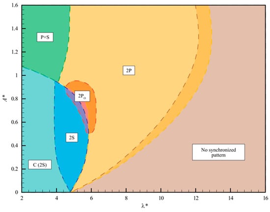
Figure 1.
Forced-vibration vortex-shedding map in normalized amplitude–wavelength space [5].
The vortex-shedding map is crucial for understanding cylinder kinematics and energy extraction for VIV generators. It provides information on energy excitation, ensuring the validity of forced-vibration experiments for free-vibration cases. Morse and Williamson [5] validated the predicting power of forced vibration by matching amplitude, frequency, and Reynolds number, which resulted in consistent fluid forces.
1.1. Related Work
Previous approaches to generating vortex-shedding maps have been reliant on gathering substantial amounts of experimental data. The vortex-shedding map shown in Figure 1 was produced through an expanded investigation that built upon the first amplitude and frequency map created by Williamson and Roshko [6]. They conducted 5680 experimental runs in a water channel, producing 500 h of data, using digital particle image velocimetry (DPIV) to visualize wake regimes with high-resolution images taken at 10- and 20-millisecond intervals. The determination of various regimes required a coupled analysis of the flow images and the fluid force measurements by the experimental apparatus. The authors used abrupt jumps in the fluid force as transitions into different regimes to define the boundaries of the shedding map. However, more complex transition states between vortex-shedding modes required investigation of the vortex phase. Generating the vortex-shedding map necessitated large amounts of data, including fluid forces and their decomposition into vortex force and potential force, alongside reference to fluid flow images of the wake. Visual inspection by an expert was necessary to manually identify spatiotemporal patterns, but this has limitations for more complex flow regimes associated with higher Reynolds numbers.
The previous studies are the extent of research in generating vortex-shedding maps and are limited to a low Reynolds number of less than 4000. The lack of investigations in generalizing the vortex-shedding behaviour in the parameter space at a higher Reynolds number may be attributed to the more complex dynamics. Wu et al. [7] studied vortex-shedding patterns from Reynolds number 35,000 to 130,000 and identified several relatively stable modes, including 2S, 2P, 2PO, P + S, and 2P + 4S. Due to instability and variations between cycles, the authors noted the inability to generalize some vortex-shedding patterns from Reynolds number 60,000 to 75,000. Zhang et al. [8] echoed this limitation at the highest free-stream turbulence intensity (5%); the vortex structure was indistinguishable in the flow field due to the large amounts of mixing from the increased dissipation energy. The authors found that the turbulence intensity of the incoming stream has a dissipation effect that causes the vortices to become weaker and increasingly difficult to distinguish.
VIV energy harvesters are expected to perform optimally in ambient airflow conditions characterized by Reynolds numbers that are greater than 4000. For instance, a mean wind velocity of 5 m/s corresponds to a Reynolds number of 10,000 [9]. The advantage of operating VIV machines in higher-Reynolds-number flows lies in the increased efficiency and energy harvesting potential resulting from increases in lift force, VIV oscillation amplitude, and synchronization range [9]. Although a vortex-shedding map at higher Reynolds numbers is beneficial, generating such a map is challenging due to high computational costs and complex dynamics, with few demonstrated methods available.
The traditional method of generating vortex-shedding maps requires large amounts of data in the form of fluid forces, resolved flow images, and visual inspection from an expert [10,11,12,13,14]. Data-driven methods for identifying and clustering distinct flow regimes from high-dimensional, time-resolved flow fields provide a versatile and automated approach to improve confidence intervals while reducing input information. Recently, in the literature, the benefits of the data-driven method of clustering on high-dimensional time-resolved flow fields have been gaining attention, specifically for identifying and grouping distinct flow dynamics of vortex shedding from VIV.
In the progression of research within this stream, our earlier publication Cann et al. [15] served as a pivotal proof of concept for validating the efficacy of the proposed clustering analysis. The paper presents an effective method of classifying 2S, 2P, and 2PO vortex structures in the wake of an oscillating circular cylinder, employing various machine-learning algorithms trained on simulated fluid flow data. An exceptional classification accuracy of 99.8% was achieved using a random forest model trained on the -component of velocity. The impressive classification results highlight the notable feature separation attainable, which is crucial for the successful unsupervised clustering of time series data. The demonstrated ability to accurately identify global vortex structures in the wake of an oscillating circular cylinder using local flow signatures provides a solid foundation for the application of the proposed clustering methods in this paper.
Clustering is a subset of unsupervised machine learning when the input data is assumed to have discrete structures that can be extracted. Unsupervised learning uses the input data structure to provide insights since there are no expert labels associated with the data. Huera-Huarte and Vernet [16] applied fuzzy clustering on digital particle image velocimetry (DPIV) data for the vortex shedding of a flexible cylinder. Proper orthogonal decomposition (POD) was used to reduce the dimensionality of the image data to identify patterns. The method adequately identified the 2S and 2P modes at two elevations along the long flexible cylinder exposed to crossflow of Reynolds numbers from 1200 to 12,000. The work by Huera-Huarte and Vernet [16] provides a pertinent application of clustering on vortex-shedding structures for an oscillating cylinder. However, the clustering analysis was only utilized to identify the 2S and 2P modes for the free-vibration experiment. The parameter space of amplitude and frequency was not explored since the experiment considered the free vibration of the cylinder. Furthermore, the entire vorticity flow field was required for clustering, despite the use of POD to reduce the data dimensions.
Menon and Mittal [17] studied pitching airfoil wake dynamics using clustering methods to identify and track vortices. The main objective of this study was to analyze the force production on the airfoil from local vortical regions using the force and moment partitioning method (FMPM). The proper application of this method requires the vortex regions near the airfoil to be accurately isolated. The authors used the clustering analysis to isolate and track the vortices primarily in the leading and trailing edge due to their overall effects on pitching airfoils. The authors used the DBSCAN clustering algorithm for the analysis based on its advantages for flow field clustering. The dataset comprises the vorticity fields from forced-vibration CFD simulations of an oscillating airfoil. The pitching frequency and amplitude parameter space were sampled extensively for the varying vortex dynamics. The authors demonstrated the utility of this methodology for the investigation of the dynamic influence of vortex-induced forces.
Another effort directed at clustering vortex-shedding modes was conducted by Calvet et al. [18] to cluster the vortex wakes of bio-inspired propulsors. The authors generated the flow fields behind an oscillating airfoil using computational fluid dynamics (CFD) at a Reynolds number of . The vorticity flow field was reduced with a deep convolutional autoencoder and clustered using -Means++. The authors selected the -Means++ algorithm after comparing the results of -Medoids, hierarchical clustering, and DBSCAN, which all showed no improvement over -Means. The combination of feature extraction and clustering based on the latent space produced an exceptional method for identifying wake kinematics. The clustering method achieved 100% accuracy in extracting airfoil wake patterns when trained on a simple one-degree-of-freedom labelled dataset, which included 2P + 4S, 2P + 2S, and 2S modes. The trained autoencoder was then applied to an unlabelled dataset of a two-degree-of-freedom oscillating airfoil with more complex modes. The optimal number of clusters for this case was determined to be six through the elbow method, silhouette index, and visual classification of the modes. The success of the authors provides a basis for the methodology used in this study, which shares similarities of developing a clustering technique for a straightforward problem of vortex shedding and extrapolating to more complex problems. However, the authors highlight the limitations of the investigation, which are linked to the input data used to train the autoencoder and clustering algorithm. Higher-amplitude vortex modes may be under-represented in the training set, potentially corrupting the results. The wake width significantly affected the clustering algorithm, indicating the need to train it to cluster based on overall vortex pattern parameters.
1.2. Objectives
In reviewing the literature, it was observed that the traditional method used for generating vortex-shedding mode maps requires large amounts of data and intensive supervision. An opportunity was identified to implement a versatile and automated data-driven approach that addresses these limitations. Furthermore, there is a lack of proposed methods for generating the vortex-shedding mode map at higher Reynolds numbers due to the increased computational cost and complex dynamics.
The main objective of this study was to develop a data-driven approach for generating vortex-shedding maps for a cylinder under forced vibration. This primary objective was discretized into two manageable goals, namely,
- Develop data-driven methods and validate their performance in the vortex-shedding map using a reference case at a low Reynolds number;
- Extend the method from Objective 1 to generate a vortex-shedding map at a higher-Reynolds-number case.
In this paper, Objective 1 was achieved by developing an unsupervised clustering method to extract a small number of well-defined clusters that are rooted in the flow physics of the low-Reynolds-number case to reproduce the benchmark vortex-shedding map. The final objective was met by generating vortex-shedding maps using the methods from Objective 1 for higher Reynolds numbers and discussing the insights gained on the underlying dynamical regimes of the physical system.
1.3. Contributions and Perspectives of This Work
The contribution of our study is twofold. First, we present a novel approach for generating vortex-shedding maps that is data-driven, automated, and accurate compared to traditional methods. Second, we demonstrate the effectiveness of our approach in handling high-Reynolds-number flow, which is a significant contribution to the field. The effort of this study deviates from previous work concerning vortex-shedding map generation by demonstrating the viability of data-driven unsupervised subsequence clustering techniques to identify vortex-shedding modes from local flow signatures sampled in the wake. Previous unsupervised clustering approaches have shown promising results for identification and dissection of vortex-shedding modes. However, these methods require extensive input data to compute the entire flow field. Furthermore, the primary contribution of this method is its use in generating vortex-shedding maps for high Reynolds numbers, which have been limited in the literature due to the increased computational cost and complex dynamics.
The data-driven approach for generating vortex-shedding maps presented in this study has the potential for several future engineering applications. One potential application is in the design and optimization of VIV wind energy harvesting systems, where accurate predictions of flow structures are essential for maximizing energy output. The current low-Reynolds-number vortex-shedding maps have limited utility in designing VIV harvesting systems that operate at higher flow speeds. By using this method, we are able to generate vortex-shedding maps for a much wider range of Reynolds numbers, which provides critical insights into the flow dynamics and aids in the design and optimization of VIV systems. The approach can also be applied to other engineering applications, such as heat exchangers, aerospace vehicles, and marine engineering, where vortex-induced vibrations can cause structural damage and impact the overall performance of the system. Moreover, the unsupervised clustering techniques employed in our approach can be extended to other fluid mechanics problems where flow structures play a significant role, such as turbulence and fluid–structure interaction.
The framework developed in this paper presents a refreshing alternative to conventional approaches for elucidating wake dynamics in the flow past a structure. This approach could lead to new and innovative designs of a new generation of energy harvesters that can exploit all forms of flow-induced vibration for energy extraction. While the methodology is tested in the paper for the more restricted case of VIV of a circular cylinder, it can be applied to a more general case of FIV in more general structures. For example, even for the cylinder–plate assembly in laminar flow (at low Reynolds numbers), the vortex-shedding map is much more complex than that produced by Morse and Williamson [5] for a circular cylinder at Re = 4000. Therefore, the framework developed in this study could provide a powerful tool for exploring and understanding the complex flow dynamics in various engineering systems, paving the way for more efficient and effective designs.
1.4. Paper Structure
The structure of this paper is as follows: Section 2 presents the vortex-shedding dataset used for clustering, Section 3 explains the novel unsupervised clustering methods, Section 4 presents the method’s performance using cluster evaluation metrics and reproduction of the benchmark vortex-shedding map, and Section 5 reports the vortex-shedding map generation performance for the clustering methods extended to a higher-Reynolds-number case. Finally, key takeaways from this investigation are provided in Section 6.
2. Vortex-Shedding Dataset
The analysis in this study requires the univariate time series signatures of local flow measurements in the wake of an oscillating circular cylinder experiencing forced vibration. The vortex shedding in a turbulent wake dataset was obtained from Kaggle [19]. The dataset was generated through 2D CFD simulations in OpenFOAMv2006 [20]. Turbulent VIV was modelled using the unsteady Reynolds-averaged Navier–Stokes (RANS) methodology, and a wall-resolved - shear stress transport (SST) turbulence closure model was employed. Furthermore, a deformable mesh was used for fluid–structure interaction to accurately capture the complex flow dynamics. The 2-dimensional domain and boundary conditions used for the numerical study are shown in Figure 2.
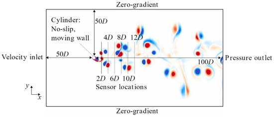
Figure 2.
Domain and boundary conditions used for the 2D simulation (not to scale).
The accuracy of 2D RANS simulations for turbulent VIV has been demonstrated in past numerical studies [21,22,23], with the - SST turbulence model performing well for separated flows with high pressure gradients common in cylinder wakes [24]. A wall-resolved approach was targeted to improve accuracy because of the effect small instabilities near the surface of the cylinder have on VIV response, with a structured, hexahedral, body-fitted mesh generated around the cylinder. The simulations were completed using the open-source finite-volume library OpenFOAMv2006 with second-order accuracy achieved in both spatial and temporal schemes. The established numerical models validated against similar experimental and computational data to replicate the vortex-shedding patterns identified by Morse and Williamson [5] provide strong evidence that the data presented in the study are of high quality and can be used with confidence in future research.
The sensor measurements are taken every 0.25 s, for 100 s, along six sampling lines located downstream in the wake of the oscillating cylinder, as shown in Figure 2. The sampling lines were orthogonal to the -axis at streamwise distances of 2, 4, 6, 8, 10, and 12, where is the cylinder diameter, and each sampling line recorded flow field measurements at 1000 locations. The data from four types of sensors were recorded from the simulations, namely, flow speed, ; the -component of velocity, ; the -component of velocity, ; and the vorticity, .
The standard fluid measurement used for wake classification is the magnitude of vorticity [25,26]. The conventional wisdom is that vorticity, a measurement of the local fluid rotation, will provide a clear signature of the rotating wakes. However, recent studies have shown that the -component of flow velocity yielded higher classification accuracy than vorticity. Alsalman et al. [27] trained several neural networks on time series data using vorticity, - and -components of flow velocity, and flow speed sensors, and found that training on the -component of velocity resulted in exceptional classification results, outperforming vorticity-trained networks even for shallow networks. The performance gain was also supported by Cann et al. [15], who demonstrated the improved accuracy of identifying vortex structures from a reduced input feature space by training machine-learning algorithms on features extracted from the frequency domain of the -component of velocity. Based on the evidence from the literature, the -component of flow velocity was used in this study to capture flow characteristics more accurately and improve the performance of the machine-learning models.
Numerous CFD simulations were conducted to provide a higher-density sampling of the parameter space investigated previously by Morse and Williamson [5]. Furthermore, the simulations were conducted at Reynolds numbers 4000 and 10,000. The Reynolds number data at 4000 were used to match the experimental setup of Morse and Williamson [5] and validate the vortex-shedding map generation procedure, referencing the benchmark map. The Reynolds number data at 10,000 were used to extend the map generation method to unknown vortex-shedding regimes. A Reynolds number of 4000 holds specific significance as it falls within the VIV regime range where turbulent vortex shedding occurs and has been identified by Wu et al. [7] as the approximate threshold at which the 2S and 2P modes emerge. Additionally, the relatively lower flow complexity at this Reynolds number allows for a comprehensive understanding of the underlying flow mechanisms. As a result, Reynolds numbers around 4000 are often selected as a benchmark value for VIV studies. The higher Reynolds number of 10,000 was chosen to maintain turbulent vortex shedding within the flow, while introducing dynamic changes to the vortex-shedding behaviour from the increased turbulence, which is not present in cases at the lower Reynolds numbers.
The study examined the impact of Reynolds number, streamwise location, and vortex-shedding modes on signal variance. Data from sampling lines and were used for clustering analysis in the low- and high-Reynolds-number cases, respectively, based on their ability to capture wake signals without significant downstream dissipation effects.
3. Unsupervised Clustering Methods
Clustering analysis is a subset of unsupervised machine learning in which a dataset is decomposed into groups, or “clusters,” based on detected shared structures in the data. The unsupervised nature of clustering means there is limited external information on the data structure other than the intrinsic properties.
A time series is a sequence of data points indexed at specific points in time, denoted , where the observation at the time, , is a subset of allowed timesteps, . The set of represents the time domain over which the time series is defined. In this application, is a set of consecutive timesteps in seconds during which the CFD simulations were conducted. There are three different types of time series clustering strategies, namely, whole time series [28], subsequence [28], and time point clustering [29]. Subsequence time series clustering was chosen for this application as it can identify specific patterns in full-time series with non-steady-state signal behaviour and isolate the desired behaviour even when multiple shedding modes are present.
3.1. Subsequence Data Mining
Subsequence time series clustering involves clustering frequent patterns in an extended time series. The frequent patterns within a time series are identified using shapelet/motif discovery techniques. The data mining community has extensively researched and developed various algorithms for time series motif discovery. Torkamani and Lohweg [29] provide a comprehensive review of these algorithms.
The time series motif extraction method for this study was conducted using the matrix profile. The matrix profile, first presented by Yeh et al. [30], is a novel algorithm for conducting a time series subsequence all-pairs similarity search. The algorithm uses a fast similarity search algorithm under -normalized Euclidean distance. The method is simple, parameter-free, and exact, implying that no false positives or false negatives are incurred in the process. The matrix profile records the distances of a subsequence with sliding window length, , to all other subsequences of the same length. The matrix profile contains two components, namely, a distance profile and a profile index. The distance profile is the vector of minimum Euclidean distance, and the profile index is the first nearest neighbour’s index. Figure 3 illustrates an example of a time series signal and its corresponding distance profile obtained from the matrix profile analysis. The distance profile in Figure 3b shows the similarity between each subsequence and all other subsequences of the same length in the time series. The blue trace in the time series highlights a motif and its nearest neighbour, which corresponds to the minimum distance value in the distance profile (marked with a red line) and profile index.
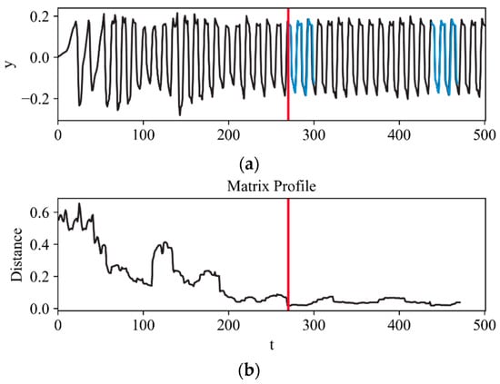
Figure 3.
Matrix profile of (a) example time series and (b) distance profile with a highlighted motif and neighbour (blue trace) identified by minimum distance profile value (red line).
Together, the time series and distance profile in Figure 3 provide a visual representation of the structure and dynamics of the time series data, allowing us to identify time series patterns and anomalies. Low distance profile values indicate similarity between subsequences within the series, corresponding to motifs, while high values indicate unique subsequences, corresponding to anomalies. The lowest values in the profile represent the prominent subsequence, which can be extracted as the motif. Careful selection of the sliding window length is crucial for domain-specific motif extraction.
3.2. Clustering Evaluation Metric
Cluster evaluation is essential for obtaining meaningful and quantifiable results. Scalar accuracy indices assess cluster quality through numerical values, consisting of internal and external indices. External indices cannot be utilized for unsupervised clustering due to the absence of external data, while internal indices use intrinsic information to determine clustering performance. The clustering quality is based on two parameters: compactness and separation. Compactness measures how close the objects within the same cluster relate to each other, known as intra-cluster similarity [31]. Separation measures how well separated a cluster is from other clusters, known as an inter-cluster similarity [31]. Many internal indices are proposed in the literature, but the silhouette and Dunn indices were selected for the evaluation metrics based on their ability to provide a measure of both intra-cluster similarity and inter-cluster dissimilarity [32].
3.2.1. Silhouette Index
The silhouette coefficient, introduced by Rousseeuw [33], measures the similarity of an element to its cluster (compactness) compared to the other sets (separation). The silhouette coefficient is determined as follows:
where the parameter is the mean distance between a sample and all the points within the same set, and the parameter is the mean distance from the sample to all the other points in the next nearest cluster. The value of the silhouette index is bounded between −1 and 1. As the silhouette approaches 1, the cluster containing the sample element will be far from the following cluster but compact within the elements of the same cluster. Negative values indicate that a sample element is closer to another cluster’s elements than to its assigned elements. The clustering analysis’s quality can be measured by calculating the average silhouette coefficient for all objects in the dataset.
3.2.2. Dunn Index
The Dunn index was first introduced by Dunn [34]. The Dunn index is the ratio of the minimum distance between clusters (inter) and the maximum distance within a cluster (intra). To quantify the Dunn index, consider any two clusters and with the corresponding members and . The Dunn index is defined as
The Dunn index should be maximized such that the minimum intercluster distance is large (separation) and the maximum intracluster distance is small (compactness).
3.3. Proposed Clustering Algorithms
The selection of clustering algorithms is crucial for clustering analysis, particularly for time series data. There are two main approaches for clustering time series data: conventional and hybrid [35]. In this study, the best-performing algorithms for clustering time series subsequences of vortex shedding were chosen, including two traditional single-step and two proposed hybrid methods.
The traditional clustering methods of -Means partitioning and agglomerative hierarchical clustering were chosen for their demonstrated performance. The -Means method was selected based on its demonstrated ability to extract highly separated clusters. The -Means algorithm was implemented using the -Means++ initialization method to select initial cluster centres that are distant, resulting in better results than random initialization by avoiding local minima [36]. The agglomerative hierarchical method was selected based on the improvements over the partitioning methods, which do not require the number of partitions to be prespecified, as the hierarchy structure can be spliced at the appropriate level to extract the clusters. The hyperparameters selected for the agglomerative algorithm were complete linkage and cosine affinity distance, which achieved the best balance of evaluation metrics.
Multi-step clustering methods, known as hybrid methods, can improve the clustering performance of traditional methods [37,38,39,40]. These methods conduct a pre-clustering phase that produces a large number of separate clusters that are then merged using a final clustering method to obtain the desired number of clusters. A reduced dataset of prototypes is used for the final clustering stage, which comprises samples extracted from the subclusters that minimize the pairwise distances between themselves and the other cluster members. The various steps involved in the proposed hybrid algorithms for clustering the motif dataset are illustrated in the flow diagram in Figure 4.
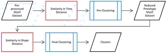
Figure 4.
Block diagram summarizing the key steps in the proposed hybrid algorithm.
Hybrid methods yield the best clustering results when the pre-clustering phase maximizes the silhouette index, indicating that the high-resolution clusters capture distinct groups. The silhouette index is expected to decrease in the final clustering stage as the clusters merge to produce more general clusters that reveal overarching patterns, leading to an increase in the Dunn index value.
Most hybrid methods use varying distance metrics for each step, usually a similarity in time distance for the pre-clustering and a shape-based similarity distance for the final clustering. The advantage of multi-step clustering is the ability to calculate the computationally expensive dynamic time warping (DTW) similarity matrix on the reduced dataset of prototypes. The clustering results obtained using the DTW distance provide an advantage for shape-based clustering analysis.
The advantage of the multi-step clustering procedure is depicted in Figure 5 using an example of clustering subsequences using a two-step hybrid method. The figure illustrates the initial subclusters’ inter-similarity based on similarity in time and the intra-similarity between the prototypes achieved in the final clustering stage.
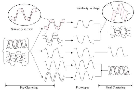
Figure 5.
Demonstration of the clustering procedure of the full subsequence set and prototype set using varying distance metrics in a two-stage hybrid clustering method.
Two hybrid methods are proposed in this study. The first hybrid method, denoted Hybrid A, uses a combination of density-based spatial clustering of applications with noise (DBSCAN) [41] and agglomerative clustering algorithms. The DBSCAN method provides an advantageous initial clustering step since the clusters are automatically determined based on the input data structures. The DBSCAN algorithm only requires two parameters, namely, the number of minimum samples and radii. These parameters represent the core samples, which are a subset of the data which include a minimum number of samples, min_samples, that are within a distance radius, . The samples that are not core and are further than distance from any core sample are considered an outlier. The agglomerative algorithm was then used to group the subclusters from the DBSCAN algorithm into the final number of clusters.
The final hybrid method proposed in this study, denoted Hybrid B, was conceptualized by combining the best-performing single-step clustering analysis into a multi-step method. The hybrid method uses the -means algorithm for the pre-clustering phase and the agglomerative method for the final clustering with the same hyperparameters as the single-step methods.
3.4. Vortex-Shedding Map Generation
The vortex-shedding maps were generated using an ensemble-type method. This method decomposed each node in the normalized amplitude–wavelength map into primary and secondary time series signatures based on the clustering results. Specifically, nodes with a strong vortex-shedding mode will have a larger proportion of time signatures clustered together in the same cluster. On the other hand, unstable nodes such as the 2PO mode, which can exhibit both 2S and 2P modes, will share multiple clusters within the node. By decomposing each node into primary and secondary time series signatures, the ensemble approach used to generate the vortex-shedding maps may allow for a more nuanced understanding of the underlying flow dynamics. The primary and secondary signatures represent the dominant and sub-dominant modes of variability in the data, respectively. The clustering methods used to identify these signatures may help to identify patterns or groups of nodes with similar flow behaviour, which could provide insights into the mechanisms that drive vortex shedding and the formation of flow patterns. The ensemble-type method is a promising approach for generating vortex-shedding maps and studying the complex flow dynamics that occur in a variety of fluid systems.
4. Vortex-Shedding Map Generation at Low Reynolds Number
This section applies the unsupervised clustering methods to a low-Reynolds-number scenario of vortex shedding from an oscillating cylinder to replicate the benchmark regime map [7]. The performance of each clustering method is evaluated based on both clustering accuracy and the quality of the resulting vortex-shedding maps.
4.1. Introduction
The following locations on the reference vortex-shedding map produced by Morse and Williamson [5] were selected to create the clustering dataset based on observed vortex-shedding behaviour in the signals.
The sampling nodes included three vortex-shedding modes (2S, 2P, and 2PO) that exhibited stable behaviour. Nodes on the frequency sampling line of 4 were excluded due to the absence of coherent patterns in the data near the C (2S) to 2S transition. The absence of a distinct transition between the C (2S) and pure 2S mode was reported as the least distinct boundary compared to any modes by Morse and Williamson [5]. The data points in the C (2S) region were carefully selected due to the small vortices that coalesce in the near wake detected by the sampling line at 6D.
The subsequences in the data were mined using the matrix profile motif extraction method. The specified window size for the algorithm was set to the equivalent of 64 timesteps to represent a total of at least two cycles of oscillation. Selecting a sliding window to capture multiple oscillations improves clustering results by producing more consistent and representative patterns. The subsequence extraction process was performed on all of the raw time series to generate a single representative pattern for clustering analysis.
The number of clusters specified in the cluster algorithms is five, considering the domain knowledge that three distinct vortex-shedding modes should be present in the data, as shown in Figure 6. The two additional clusters were designated for separating transitional modes such as 2PO and any noise or outlier points identified in the clustering procedure.
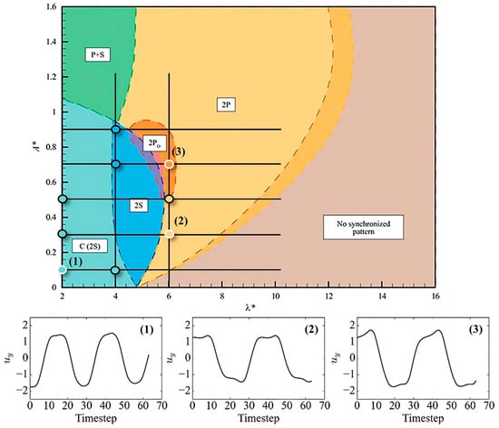
Figure 6.
Dataset sampled nodes overlaid reference normalized amplitude () –wavelength () plane [5], with three subpanels showing example signals extracted from each corresponding node on map, denoted 1, 2, and 3.
4.2. k-Means
The first clustering method implemented to cluster time series subsequences was the -Means algorithm. The internal metrics of the silhouette and Dunn indices were employed to evaluate the clustering performance, and the results are summarized in Table 1.

Table 1.
Clustering performance metrics of -Means method at Re = 4000.
The relatively high evaluation metrics indicate that the clusters generated are sufficiently separate and compact, which can visually be confirmed by the time series subsequence clusters shown in Figure 7.
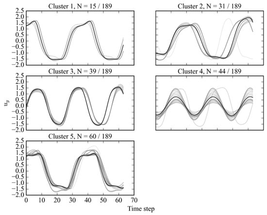
Figure 7.
Subsequence dataset clustered by -Means method at Re = 4000, with representing the number of samples in each cluster relative to the total dataset.
The similarities of cluster 1 and cluster 5 are illustrated in Figure 7, both clusters exhibiting a double-peak behaviour synonymous with the 2P group. However, the algorithm identified a subtle ramping of the peak in cluster 1, which is characteristic of the 2PO mode. The vortex-shedding map was then plotted with the primary cluster candidates identified, as shown in Figure 8.
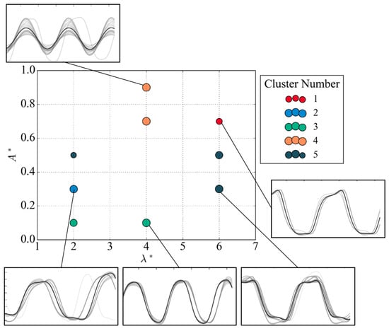
Figure 8.
Vortex-shedding map using -Means method at Re = 4000.
The generated vortex-shedding map identifies several regions of interest, with cluster 1 designated to the node at = (6, 0.7) resembling a 2PO mode with a reduced first peak in the pattern. Cluster 2 is primarily for the low-frequency case , which occurs mainly at and as the secondary mode at . The low-amplitude, , space exhibits the regular sinusoidal pattern indicative of 2S behaviour under the identification of cluster 3. A similar sinusoidal pattern is observed with cluster 4, differing by a lower signal amplitude. Finally, cluster 5 is primarily located at at with an additional split located at = (2, 0.5). The additional node shows a rather weak identification due to the switching between cluster 5 and cluster 2.
4.3. Agglomerative
The following clustering algorithm implemented was the agglomerative hierarchical algorithm. The internal indices used to quantify the clustering performance are summarized in Table 2.
Table 2.
Clustering performance metrics of agglomerative method at Re = 4000.
The agglomerative method produces clusters with a much larger Dunn index compared to the partitioning method, indicating the quality of the groups, which can be seen by the distinct clusters shown in Figure 9.
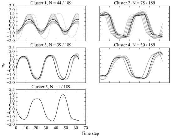
Figure 9.
Subsequence dataset clustered by agglomerative (complete, cosine) method at Re = 4000, with representing the number of samples in each cluster relative to the total dataset.
The cluster diagram in Figure 9 displays the distinctiveness of the generated clusters, particularly clusters 2, 3, and 4. However, cluster 5 appears to inhabit the same subspace as cluster 1, potentially due to its higher amplitude and longer wavelength. Despite this, the vortex-shedding map clearly illustrates the primary cluster candidates, as shown in Figure 10.
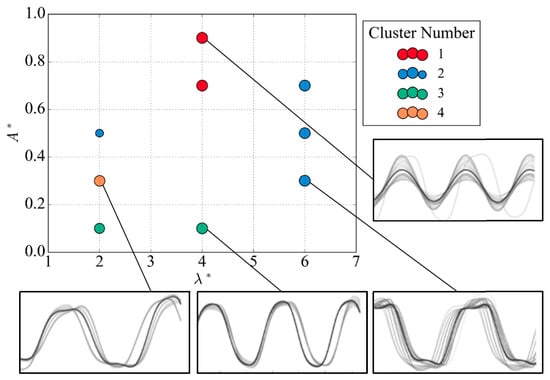
Figure 10.
Vortex-shedding map using the agglomerative method at Re = 4000.
The vortex-shedding map isolates several similar regions of subsequence patterns, consistent with those observed in the -Means method. Additionally, clusters 1 and 3 exhibit patterns similar to the signature expected for the 2S mode, while a group of nodes identified as cluster 2 on the sampling line 6 demonstrates the double peak of the pair of vortices being shed from the 2P mode.
4.4. Hybrid A
The clustering analysis results are presented for the corresponding phases using DBSCAN as the pre-clustering phase and agglomerative for the final merging of clusters. The pre-clustering phase identified six clusters, with three outliers, and a prototype was created for each cluster, which was used for the final clustering stage. The clustering performance results of both phases are summarized in Table 3.
Table 3.
Clustering performance metrics of Hybrid A method at Re = 4000.
The DBSCAN algorithm in the pre-clustering phase produced well-separated clusters resulting in a high silhouette index. The final merging step improved the Dunn index marginally at the cost of a slight reduction of the silhouette index. The generated clusters merged for the entire dataset are shown in Figure 11.
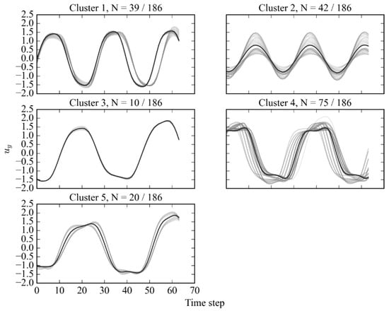
Figure 11.
Subsequence dataset clustered by Hybrid A method at Re = 4000, with representing the number of samples in each cluster relative to the total dataset.
The associated vortex-shedding map was generated based on the primary cluster candidates and the proportions of cluster samples at each node shown in Figure 12.
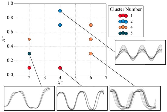
Figure 12.
Vortex-shedding map using Hybrid A method at Re = 4000.
Using the Hybrid A method, the generated regime map shares its overall structure with the other methods. Specifically, the nodes along the line 6 all belong to the primary mode identified in cluster 4 that resembles the 2P mode. The low amplitude nodes along the horizontal line share cluster 1. The sinusoidal mode with a lower amplitude is located at = (4, 0.7) and = (4, 0.9). Finally, the node located at = (2, 0.5) comprises two modes labelled by cluster 4 and cluster 3.
4.5. Hybrid B
This section presents results for the pre-clustering and final clustering phases of the last proposed hybrid method. In the pre-clustering phase, the -Means algorithm requires the optimum number of clusters to maximize the silhouette index. The optimum number of clusters for the pre-clustering phase was 20 as it maximized the silhouette index, representing well-separated clusters. The clustering performance of both phases is summarized in Table 4.
Table 4.
Clustering performance metrics of Hybrid B method at Re = 4000.
The evaluation metrics indicate significantly separated clusters in the first stage and more general clusters merged in the final stage observed by the decrease in the silhouette index but an improvement to the Dunn index. The final clusters merged for the entire dataset are shown in Figure 13.
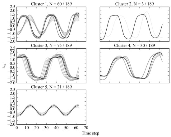
Figure 13.
Subsequence dataset clustered by Hybrid B method at Re = 4000, with representing the number of samples in each cluster relative to the total dataset.
Overall, the clusters capture distinct subsequence patterns. However, the low number of samples in cluster 2 and signal variation in cluster 1 could be responsible for the relatively poor performance of the Dunn index. The generated vortex-shedding map is shown in Figure 14 for the respective cluster candidate proportions.
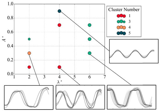
Figure 14.
Vortex-shedding map using Hybrid B method at Re = 4000.
The vortex-shedding map exhibits a similar structure to the regime map generated using the Hybrid A method. For example, the nodes along the line 6 are indicative to the 2P and 2P0 modes. The sinusoidal signals of clusters 1 and 5 are located in similar locations to the prior hybrid method results. These results provide further validation of the effectiveness of the proposed hybrid method.
4.6. Discussion
Each clustering method offers varying benefits to the unsupervised clustering task, and their respective performance and qualitative attributes are discussed in this section, culminating in an assessment of their suitability for producing vortex-shedding maps. The clustering method’s ability to produce separate and compact clusters was accessed by the internal evaluation metrics summarized in Table 5.
Table 5.
Final clustering performance metrics of proposed methods at Re = 4000.
The -Means method is beneficial for implementation due to its simple algorithm and linear time complexity. However, the requirement to specify the number of clusters and the assumption of spherical cluster shape can impact performance for the application of generating vortex-shedding maps. Hierarchical methods offer benefits such as not requiring the number of clusters to be specified and great visualization power but have drawbacks such as increased computational complexity and the inability to reassign samples once merged. The hierarchical agglomerative algorithm outperforms the partitioning method in both the silhouette and Dunn indices. However, maximizing the Dunn index can result in few samples being clustered together, which affects generalizability. Nevertheless, the agglomerative algorithm’s clustering performance is still competitive and is considered for high-Reynolds-number cases.
The single-step methods using traditional clustering are validated in the generation of vortex-shedding maps by comparing them to the reference map [5]. The vortex-shedding map produced using the -Means method is overlaid with the regimes in the reference map as shown in Figure 15. The coloured ellipses in the figure are used purely for the purpose of visualizing regions of similar vortex-shedding behaviour; the size and orientation of the ellipses were arbitrarily determined to convey a sense of these regions.
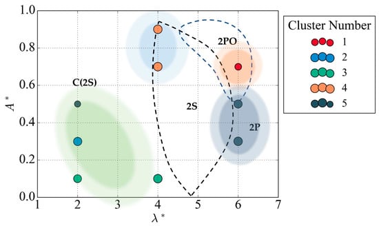
Figure 15.
Overlaid benchmark regimes on vortex-shedding map produced with k-Means.
The -Means method produced groups that align with the expected regimes established by Morse and Williamson [5]. Specifically, the algorithm identified a cluster solely associated with the 2PO mode. Clusters 4 and 5 exclusively inhabit the 2S and 2P modes on the benchmark map, with the assigned cluster numbers showing more variation in the C (2S) region. The nodes located in this region at low values of non-dimensional amplitude are strongly controlled by the clear sinusoidal cluster of number 3. The vortex-shedding map produced using the agglomerative algorithm is overlaid with the regimes in the reference map as shown in Figure 16.
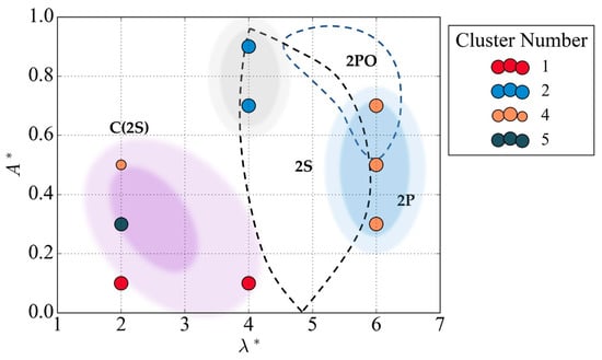
Figure 16.
Overlaid benchmark regimes on vortex-shedding map produced with agglomerative algorithm.
Clusters 2 and 4 identify general regions fitting the expected modes of 2P and 2S, respectively. It is not surprising that cluster 4 is designated in the 2PO region, as the vortex-shedding behaviour of 2PO is similar to 2P and can switch intermittently.
This paper proposes two hybrid clustering methods with varying attributes and inherent limitations. Hybrid A method combines DBSCAN and agglomerative clustering, leveraging DBSCAN’s ability to define highly separated clusters and identify outliers with unbounded parameters. Another advantage of incorporating DBSCAN is the reduced complexity in the parameter initialization, as it eliminates the need to specify the number of partitions.
The Hybrid B method was specifically developed to optimize the clustering performance based on the results of single-stage clustering analysis, combining the clustering algorithms -Means and agglomerative. The -Means algorithm offers several advantages, including easy implementation due to its relatively simple algorithm and linear time complexity, denoted as , where represents the number of data objects [42]. However, the -Means algorithm requires the initialization of the number of clusters, which poses a limitation in this data-driven study due to the absence of domain knowledge. Additionally, the -Means algorithm is sensitive to input data, initial seeds, and outliers, primarily due to the crucial step of initializing the cluster centres.
Both methods share the advantages and drawbacks associated with hierarchical clustering techniques employed for final clustering. One significant advantage is the flexibility in determining the number of the partitions, as the hierarchy structure can be spliced at the appropriate level to extract the clusters. However, hierarchical methods also have limitations that can impact clustering performance. For instance, the computational complexity of agglomerative algorithms is considered quadratic, [43], which hampers scalability for larger datasets. Additionally, the sequential approach of merging clusters in the algorithm restricts the reassignment of samples once they are merged.
Hybrid A outperforms Hybrid B in terms of silhouette and Dunn indices, showing a 31.8% and 255% increase, respectively. The high silhouette index demonstrates DBSCAN’s proficiency in creating well-defined clusters and removing noise points in the subspace. Incorporating agglomeration in the final clustering stage results in a slightly enhanced Dunn index, generating more comprehensive clusters. To validate the accuracy of the hybrid method’s ability to create vortex-shedding maps, a comparison was made with the reference map generated by Morse and Williamson [5]. Figure 17 illustrates the vortex-shedding map produced using Hybrid A overlaid with the reference map’s regimes.
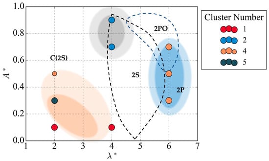
Figure 17.
Overlaid benchmark regimes on vortex-shedding map produced with Hybrid A.
The identified clusters are in line with the expected regions from Morse and Williamson [5], with cluster 2 and cluster 4 points corresponding to the pure 2S and 2P regions, respectively. While the 2PO mode does not have a distinct cluster identification, vortex-shedding patterns at this node can exhibit both pure 2P signals and intermittent 2PO modes. Similar to all of the clustering methods presented, variation in the groups of clusters in the C (2S) regime is observed. Cluster 1 strictly shows a regular sinusoidal pattern at low values of non-dimensional amplitude . The clusters identified at locations ( = (2, 0.3) and ( = (2, 0.5) show an unexpected 2P mode.
This common theme of unexpected 2P mode signals identified by the clustering techniques in the C (2S) region may be attributed to the flow physics at this low-wavelength case. The C (2S) mode is described by its synchronized 2S mode comprising small vortices that coalesce in the near wake, forming large-scale structures downstream. This coalescence and transformation of small vortical structures in the streamwise direction corrupt the patterns in the data. In conclusion, the results of the data-driven methods for generating vortex-shedding maps were determined to agree with the benchmark regime map produced by Morse and Williamson [5]. The regime maps and corresponding clusters reveal the underlying signatures of each mode based only on the local flow measurements of the -component of velocity. The cluster candidates used to plot the regime map provided more precise distinctions between the modes with a satisfactory agreement with the reference map, validating the use of clustering methods for generating vortex-shedding maps for an oscillating cylinder at low Reynolds numbers. This section achieved its objective of implementing a data-driven approach requiring less input data and supervision, relying solely on local flow measurements and unsupervised clustering. The clustering methods presented in this section are extended to produce vortex-shedding maps for high Reynolds numbers and more complex vortex structures, which can be difficult to discern using traditional methods.
5. Vortex-Shedding Map Generation at High Reynolds Number
This section applies unsupervised clustering methods validated in Section 4 for the low-Reynolds-number case to a higher-Reynolds-number case to produce a vortex-shedding map for more complex flow regimes. The performance of each clustering method is evaluated based on both clustering accuracy and the quality of the resulting vortex-shedding maps.
5.1. Introduction
This section presents the application of the validated unsupervised clustering strategies to a case of high Reynolds number where the mapped domain is unknown to gain insights into the complex flow regimes. The quality of the clustering analysis was evaluated using internal clustering metrics, visual analysis of the clusters, and finally exploring the patterns of the generated vortex-shedding maps. The main contributions of this section include gaining insights into the underlying dynamical regimes of the vortex shedding through map generation. Moreover, we also quantify the clustering performance to extract meaningful patterns from the local flow field experiencing increased instability and mixing due to the increased dissipation in the energy of the flow.
The high-Reynolds-number dataset [19] sampled the normalized amplitude–wavelength plane of forced oscillations along five sampling lines. A subset of nodes was identified as suitable for the clustering analysis based on the exhibited stable and synchronized vortex-shedding behaviour. Nodes that did not exhibit stable vortex-shedding behaviour or showed no synchronized pattern were excluded from the analysis to avoid adding noise to the dataset. The nodes selected for the cluster analysis based on these features are shown in Figure 18.
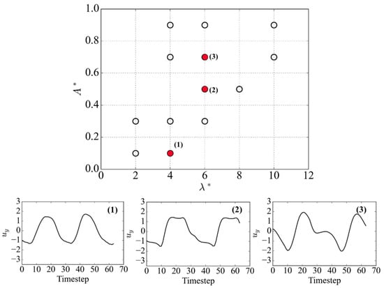
Figure 18.
Dataset sampled nodes in the normalized amplitude ()–wavelength () plane, with subpanels showing example signals extracted from each corresponding node on the map, denoted 1, 2, and 3.
The repeated patterns in the local flow measurements were then isolated using the subsequence extraction method. The quality of extracted subsequences for the high-Reynolds-number cases is pivotal in the clustering results since more fluctuating signals are observed. The window size used for the matrix profile algorithm was confirmed for applying the high-Reynolds-number case by visual inspection of a relatively consistent pattern shown in Figure 19.
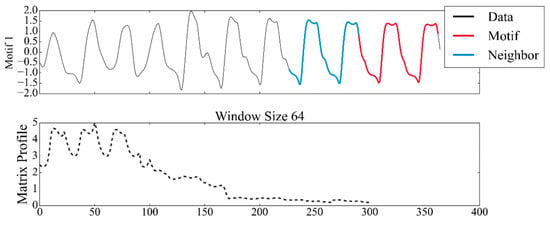
Figure 19.
Motif extraction for high-Reynolds-number signals of consistent pattern observed at () = (0.5, 6).
The window size of 64 extracts meaningful patterns from the sample signal even with unstable signals. Smaller window sizes would not capture the repeated global patterns, and larger window sizes would not extract valuable patterns to aid in the clustering analysis. Applying the clustering methods selected from the low-Reynolds-number cases requires the number of clusters to be specified. Since this study limits the domain knowledge required for map generation, the optimum number of clusters must be determined. The number of clusters should optimize the clustering performance and the insights that can be extracted through clustering. To ensure that the generated clusters can provide value in the map generation, a limit of 10 clusters is specified. The upper bound adheres to the rule of thumb in cluster analysis, which approximates the number of clusters using the formula for a training dataset of instances [44], which yields an estimated limit of 11 clusters.
5.2. k-Means
The first step in implementing the -Means method was determining the number of clusters to consider for this case. Based on the balance of the silhouette and Dunn indices, nine clusters were ultimately chosen. By balancing these metrics, we were able to select a suitable number of both internally cohesive and well-separated clusters that allowed for the clear identification of stable vortex-shedding signals while avoiding overfitting or underfitting the data. The -Means method validated in the previous section was implemented using the same initialization method of -Means++. The clustering performance for the high-Reynolds-number case was quantified using the internal metrics summarized in Table 6.
Table 6.
Clustering performance metrics of -Means method at Re = 10,000.
The evaluation metrics of the clusters indicate a good balance of high silhouette and Dunn indices, implying that the clusters are both distinct from one another and internally homogeneous. The corresponding clusters generated are shown in Figure 20.
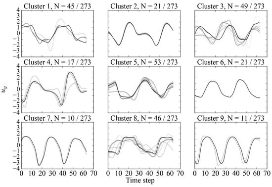
Figure 20.
Subsequence dataset clustered by -Means method at Re = 10,000, with representing the number of samples in each cluster relative to the total dataset.
From the generated clusters, some patterns begin to appear. Clusters 7 and 9 both exhibit a regular sinusoidal variation with prominent peaks and troughs in the signal. A similar pattern with low amplitude is observed in cluster 6. The expected pattern of the 2PO mode is observed in cluster 2 and cluster 4, highlighted by a smaller peak in between the peaks. More irregular signals are highlighted in clusters 1, 3, 5, and 8. Despite the variations in the signals of clusters 1 and 8, an underlying pattern persists of smaller dual peaks. Clusters 3 and 5 exhibit a regular, albeit smaller-amplitude, sinusoidal variation of the clusters.
5.3. Agglomerative
The validated agglomerative method uses the same complete linkage and cosine affinity distance as that used for the low-Reynolds-number case. The internal indices used to quantify the clustering performance are summarized in Table 7.
Table 7.
Clustering performance metrics of agglomerative method at Re = 10,000.
The clusters associated with the evaluation metrics are shown in Figure 21.
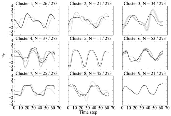
Figure 21.
Subsequence dataset clustered by agglomerative (complete, cosine) method at Re = 10,000, with representing the number of samples in each cluster relative to the total dataset.
The clusters generated using the agglomerative procedure share many similarities with the clusters of the -Means method. A sub-peak in between cycles is synonymous with the 2PO mode and is identified in clusters 1 and 3. Pure modes were identified in clusters 1, 3, 5, 7, and 9, with slight variation in the samples. Inconsistent patterns are observed in clusters 4 and 5, where the clusters would benefit from additional merging.
5.4. Hybrid A
The hybrid methods validated in the low-Reynolds-number case are compared based on internal evaluation metrics, cluster plots, and the generated vortex-shedding map. The number of clusters in the pre-clustering phase is not required to be determined since the DBSCAN algorithm automatically finds the optimum number and corresponding noise points. The algorithm found 14 separate clusters and 30 noise points. The clustering performance results of both phases are summarized in Table 8.
Table 8.
Clustering performance metrics of Hybrid A method at Re = 10,000.
The generated clusters merged for the entire dataset are shown in Figure 22.
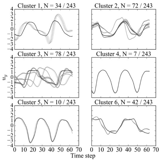
Figure 22.
Subsequence dataset clustered by Hybrid A method at Re = 10,000, with representing the number of samples in each cluster relative to the total dataset.
The cluster samples in each label demonstrated the hybrid method B’s ability to extract similar shape patterns. Cluster 3 contains out-of-phase samples, but the similarity in shape is observed between the patterns.
5.5. Hybrid B
The pre-clustering phase involved determining the optimum number of clusters, which was achieved by selecting the number that maximized the silhouette index. Through this approach, the optimal number of clusters was found to be 30, as it maximized the separation of the clusters in the first stage. The clustering performance results of both phases are summarized in Table 9.
Table 9.
Clustering performance metrics of Hybrid B method at Re = 10,000.
In the final cluster phase, the merged cluster labels produced the subsequence clusters shown in Figure 23.
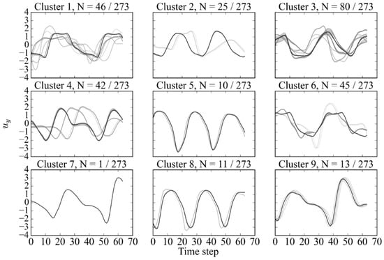
Figure 23.
Subsequence dataset clustered by Hybrid B method at Re = 10,000, with representing the number of samples in each cluster relative to the total dataset.
The patterns of interest in the generated clusters include the resemblance of a 2S mode for clusters 5 and 8. Clusters 1, 3, and 6 include more irregular signals, but an underlying pattern of smaller dual peaks can be distinguished. Finally, cluster numbers 4, 7, and 9 exhibit strong 2PO behaviour.
5.6. Discussion
The validated clustering methods were implemented for the case of a high Reynolds number. The clustering method’s ability to produce separate and compact clusters was accessed by the internal evaluation metrics summarized in Table 10.
Table 10.
Final clustering performance metrics of proposed methods at Re = 10,000.
In terms of the evaluation metrics of the silhouette and Dunn indices, the single-stage clustering methods performed better than the hybrid methods. The reduced clustering performance of the hybrid methods is attributed to the use of dynamic time warping (DTW) in the final clustering phase, which groups signals based on shape rather than time. The pairwise distance calculation in the silhouette and Dunn indices will score time series poorly if the patterns are out of phase, even if the shape is similar in the cluster.
However, the clusters produced using the hybrid methods are more similar based on shape than the single-stage methods. The similarity in shape of the hybrid methods will yield better vortex-shedding maps based on signature shapes. The improved vortex-shedding maps are observed in the plotted domain of non-dimensional amplitude and wavelength. The maps generated using the traditional methods display more scattered and irregular patterns, which results in the need for a larger number of clusters to capture the full range of vortex-shedding behaviour. In contrast, the proposed ensemble method produces more coherent and consistent maps, allowing for a more comprehensive understanding of the flow dynamics with a smaller number of clusters.
Despite the lower overall evaluation metrics, it was determined that hybrid methods outperformed single-stage methods in the quality of the clusters based on the similarity of shape and the lower number of clusters required to represent the data. The various regions of vortex-shedding behaviour at high Reynolds numbers can be obtained by analyzing the produced cluster maps. The non-dimensional amplitude and wavelength plane populated with the corresponding clusters derived using Hybrid A method is shown in Figure 24.
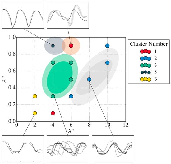
Figure 24.
Vortex-shedding map regions using the Hybrid A method at Re = 10,000.
The coloured regions only visualize similar vortex-shedding behaviour determined by cluster number. Two independent regions are located at the top of the map, = (4, 0.9) and = (6, 0.9), with consistent vortex-shedding signals. The former node signal is periodic with distinct peaks that resemble the 2S mode. The second node signal, denoted with cluster number 1, indicates the 2PO mode with a subpeak in between the relative peaks generated by the weaker vortex structure. The samples in cluster 1 include samples closer to that of cluster 5 located at the previous node, which indicates a level of overlap between the vortex structures. A larger group of nodes with the same cluster number was identified in the middle of the map, and . Cluster 3 follows differing variations of 2PO and 2P of dual peak and sub-peaks in oscillating actions. The region defined by cluster 2 resembles the signal of the P + S mode determined from the smoothed dual peak of the oppositely signed vortices of the P mode and the single peak of the S mode passing the sensor.
The cluster map produced using the Hybrid B method also outlines various regions of similar fluid flow behaviour. The vortex-shedding map populated with the corresponding clusters derived using the Hybrid B method is shown in Figure 25.
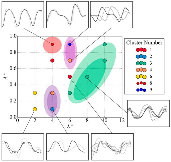
Figure 25.
Vortex-shedding map regions using the Hybrid B method at Re = 10,000.
The coherent vortex-shedding patterns identified in the map first include the 2S behaviour at the node = (4, 0.9). Nearby, two strong 2PO clusters were identified at = (6, 0.9) and = (4, 0.7), demonstrated by a weaker vortex being shed in between the oscillations. The former point of cluster 9 shares the similarity in shape but at high peak amplitudes compared to cluster 4. The largest region of similar behaviour is identified by cluster 3, which dominates the higher wavelength portion of the subspace. The signals in cluster 3 demonstrate the behaviour of 2P but appear to have less defined twin peaks. Finally, a region in low-amplitude nodes was identified resembling the 2S mode at lower amplitudes compared to that of node = (4, 0.9).
From a flow physics perspective, the vortex-shedding maps at high Reynolds numbers provide novel insights into the underlying vortex–structure interactions. The higher Reynolds number and associated higher flow energy seemed to produce more variation signals and a stronger dissipation effect. The dissipation effect is a product of a more turbulent flow, which increases flow mixing and creates a more homogenous flow. The signals appeared smooth, with samples with twin peaks not as defined as the low-Reynolds-number case at 4000. Furthermore, the high Reynolds number was observed to create more noise in the vortex-shedding map with an increased number of nodes with no visible patterns due to the coalescence of vortices. Overall, the signals of the high-Reynolds-number case were of the larger amplitude of the -component of velocity measurement. Specifically, the 2S behaviour showed large amplitudes between peaks in the signals, which aided in identifying these clusters.
The high-Reynolds-number case has clear regions of the 2PO mode demonstrated by the signals of clusters 4 and 9, which show the two pairs of vortices being shed per cycle with one vortex in each oscillation much weaker. The transition mode is in close proximity to the observed P + S signal behaviour of cluster 3 demonstrated by the dual peak of the P mode being separated with a single peak from the S mode. The source of the P + S mode may be attributed to the increased turbulent kinetic energy of a high Reynolds number, which is decomposing 2P modes shed close to the cylinder into a single P and S mode. The devolution of the 2P mode would have to be rapid as the sampling line of the dataset is located at a distance of 4D in the wake of the cylinder. If the decomposition of the 2P mode is the mechanism in which the P + S mode appears in the dataset, it would have a negligible impact on the overall behaviour of the cylinder. The negligible impact is because the observed rapid decay implies that the P + S mode dissipates quickly and does not contribute significantly to the long-term vortex-shedding dynamics of the cylinder.
In conclusion, Hybrid A and B methods were found to be the most effective in generating clusters with high similarity of shape, outperforming the single-stage methods. The vortex-shedding maps produced by these hybrid methods reveal valuable information about the system’s dynamics. Notably, the Reynolds number case of 10,000 exhibits similar vortex-shedding modes as the low-Reynolds-number dataset, including the 2S and 2PO modes. The region of the map previously inhabited with 2P modes was observed to comprise the majority of P + S modes. Overall, the flow physics derived from the cluster analysis demonstrates the increased dissipation effect in a high Reynolds flow, resulting in a smoothing effect on the flow signals.
6. Conclusions
This study developed a data-driven approach for generating vortex-shedding maps of a circular cylinder undergoing forced vibration. The unsupervised clustering of local flow measurement time series subsequences reproduced the benchmark vortex-shedding map at Reynolds number 4000. The clustering method developed herein was then applied to a high-Reynolds-number flow to generate a vortex-shedding map that had not previously existed.
The procedure of generating vortex-shedding maps using novel unsupervised subsequence clustering methods was presented and validated for the case of a low Reynolds number of 4000 in Section 4. Several clustering methods were selected and compared for the clustering task of subsequences extracted from the -component of the velocity () time series data. The clustering results of the proposed methods demonstrated their ability to extract meaningful clusters that represented the underlying flow physics of the varying modes. The application of the clustering analysis to produce regime maps provided satisfactory agreement with the reference map by Morse and Williamson [5].
The proposed methods were then extended in Section 5 to quantify their performance to produce vortex-shedding maps at high Reynolds numbers with more complex vortex structures. The hybrid methods were the most effective in generating clusters with high similarity of shape, outperforming the single-stage methods. The vortex-shedding maps produced at a high Reynolds number provided novel insights into the underlying vortex structure interactions and identified numerous regions of similar patterns despite increased instability. The clustering procedure in the generation of vortex-shedding maps offers a method that requires less data and supervision without resolving the entire flow field. The method was implemented on the vortex-shedding patterns of an oscillating cylinder, but the method could create value for any vortex-shedding behaviour.
Possible future work for this study includes a more comprehensive sampling of the normalized amplitude–wavelength plane, specifically in the transition zones, to provide a higher resolution of the cluster regions. Furthermore, incorporating real-world experimental data or higher resolution numerical data derived from large-eddy simulations (LES) to validate and expand upon our results would also be valuable, enabling a more robust assessment of the procedure. Optimizing the computational efficiency of the proposed clustering approach and exploring its generalizability to different geometric configurations, flow conditions, and Reynolds numbers would enhance its applicability. Furthermore, integrating the clustering results into system design and optimization processes would provide insights into the impact of different flow regimes on the efficiency and stability of VIV wind energy harvesting systems.
Author Contributions
Conceptualization, M.C.; methodology, M.C.; software, M.C.; validation, M.C. and R.M.; formal analysis, M.C.; investigation, R.M.; resources, F.-S.L.; data curation, R.M.; writing—original draft preparation, M.C.; writing—review and editing, M.C. and E.Y.; visualization, M.C. and R.M.; supervision, F.-S.L. and W.M.; project administration, F.-S.L. and W.M.; funding acquisition, F.-S.L. All authors have read and agreed to the published version of the manuscript.
Funding
This research was funded by the Natural Sciences and Engineering Research Council of Canada (NSERC) Discovery Grants program Grant Nos. 50503-10234 and 50503-10925.
Data Availability Statement
Research data generated during this study that support the reported results can be found at https://www.kaggle.com/datasets/ryleymcconkey/vortex-shedding-wake (accessed on 16 October 2021).
Conflicts of Interest
The authors declare no conflict of interest.
References
- Fan, D.; Wu, B.; Bachina, D.; Triantafyllou, M.S. Vortex-induced vibration of a piggyback pipeline half buried in the seabed. J. Sound Vib. 2019, 449, 182–195. [Google Scholar] [CrossRef]
- Kumar, N.; Kolahalam, V.K.V.; Kantharaj, M.; Manda, S. Suppression of vortex-induced vibrations using flexible shrouding—An experimental study. J. Fluids Struct. 2018, 81, 479–491. [Google Scholar] [CrossRef]
- Wang, W.; Wang, X.; Hua, X.; Song, G.; Chen, Z. Vibration control of vortex-induced vibrations of a bridge deck by a single-side pounding tuned mass damper. Eng. Struct. 2018, 173, 61–75. [Google Scholar] [CrossRef]
- Wu, Y.; Cheng, Z.; McConkey, R.; Lien, F.-S.; Yee, E. Modelling of Flow-Induced Vibration of Bluff Bodies: A Comprehensive Survey and Future Prospects. Energies 2022, 15, 8719. [Google Scholar] [CrossRef]
- Morse, T.L.; Williamson, C.H.K. Fluid forcing, wake modes, and transitions for a cylinder undergoing controlled oscillations. J. Fluids Struct. 2009, 25, 697–712. [Google Scholar] [CrossRef]
- Williamson, C.H.K.; Roshko, A. Vortex formation in the wake of an oscillating cylinder. J. Fluids Struct. 1988, 2, 355–381. [Google Scholar] [CrossRef]
- Wu, W.; Bernitsas, M.M.; Maki, K. RANS Simulation Versus Experiments of Flow Induced Motion of Circular Cylinder With Passive Turbulence Control at 35,000 < Re < 130,000. J. Offshore Mech. Arct. Eng. 2014, 136, 041802. [Google Scholar] [CrossRef]
- Zhang, D.; Wang, W.; Sun, H.; Bernitsas, M.M. Influence of turbulence intensity on vortex pattern for a rigid cylinder with turbulence stimulation in flow induced oscillations. Ocean Eng. 2021, 237, 109349. [Google Scholar] [CrossRef]
- Bernitsas, M.; Ben-Simon, Y.; Raghavan, K.; Garcia, E. The VIVACE Converter: Model tests at high damping and Reynolds number around 105. J. Offshore Mech. Arct. Eng. 2009, 131, 011102. [Google Scholar] [CrossRef]
- Païdoussis, M.P.; Price, S.J.; de Langre, E. 3. Vortex-Induced Vibrations. In Fluid-Structure Interactions—Cross-Flow-Induced Instabilities; Cambridge University Press: Cambridge, UK, 2010; Available online: https://app.knovel.com/hotlink/pdf/id:kt008NA8H1/fluid-structure-interactions/two-dimensional-viv-phenomenology (accessed on 25 October 2021).
- Techet, A. “13.42 Lecture: Vortex Induced Vibrations,” MIT OCW, Apr. 21, 2005. Available online: https://ocw.mit.edu/courses/mechanical-engineering/2-22-design-principles-for-ocean-vehicles-13-42-spring-2005/readings/lec20_viv1.pdf (accessed on 18 October 2021).
- Triantafyllou, M.S.; Bourguet, R.; Dahl, J.; Modarres-Sadeghi, Y. Vortex-Induced Vibrations In Springer Handbook of Ocean Engineering, 1st ed.; Springer International Publishing: Berlin/Heidelberg, Germany, 2016; pp. 819–850. [Google Scholar]
- Yang, W.; Masroor, E.; Stremler, M.A. The wake of a transversely oscillating circular cylinder in a flowing soap film at low Reynolds number. J. Fluids Struct. 2021, 105, 103343. [Google Scholar] [CrossRef]
- Williamson, C.H.K.; Govardhan, R. Vortex-induced vibrations. Annu. Rev. Fluid Mech. 2004, 36, 413–455. [Google Scholar] [CrossRef]
- Cann, M.; McConkey, R.; Lien, F.-S.; Melek, W.; Yee, E. Mode classification for vortex shedding from an oscillating wind turbine using machine learning. J. Phys. Conf. Ser. 2021, 2141, 12009. [Google Scholar] [CrossRef]
- Huera-Huarte, F.J.; Vernet, A. Vortex modes in the wake of an oscillating long flexible cylinder combining POD and fuzzy clustering. Exp. Fluids 2010, 48, 999–1013. [Google Scholar] [CrossRef]
- Menon, K.; Mittal, R. Quantitative analysis of the kinematics and induced aerodynamic loading of individual vortices in vortex-dominated flows: A computation and data-driven approach. J. Comput. Phys. 2021, 443, 110515. [Google Scholar] [CrossRef]
- Calvet, A.G.; Dave, M.; Franck, J.A. Unsupervised clustering and performance prediction of vortex wakes from bio-inspired propulsors. Bioinspir. Biomim. 2021, 16, 046015. [Google Scholar] [CrossRef]
- McConkey, R. Vortex Shedding in a Turbulent Wake. Available online: https://www.kaggle.com/ryleymcconkey/vortex-shedding-wake (accessed on 16 October 2021).
- ESI OpenCFD Releases OpenFOAM v2006. Available online: https://www.openfoam.com/news/main-news/openfoam-v20-06 (accessed on 27 April 2023).
- Kinaci, O. 2-D URANS Simulations of Vortex Induced Vibrations of Circular Cylinder at Trsl3 Flow Regime. J. Appl. Fluid Mech. 2016, 9, 2537–2544. [Google Scholar] [CrossRef]
- Khan, N.B.; Ibrahim, Z.; Nguyen, L.T.T.; Javed, M.F.; Jameel, M. Numerical investigation of the vortex-induced vibration of an elastically mounted circular cylinder at high Reynolds number (Re = 104) and low mass ratio using the RANS code. PLoS ONE 2017, 12, e0185832. [Google Scholar] [CrossRef] [PubMed]
- Zhao, M.; Cheng, L. Vortex-induced vibration of a circular cylinder of finite length. Phys. Fluids 2014, 26, 015111. [Google Scholar] [CrossRef]
- Menter, F.R. Two-equation eddy-viscosity turbulence models for engineering applications. AIAA J. 1994, 32, 1598–1605. [Google Scholar] [CrossRef]
- Colvert, B.; Alsalman, M.; Kanso, E. Classifying vortex wakes using neural networks. Bioinspir. Biomim. 2018, 13, 025003. [Google Scholar] [CrossRef]
- Wang, M.; Hemati, M.S. Detecting exotic wakes with hydrodynamic sensors. Theor. Comput. Fluid Dyn. 2019, 33, 235–254. [Google Scholar] [CrossRef]
- Alsalman, M.; Colvert, B.; Kanso, E. Training bioinspired sensors to classify flows. Bioinspir. Biomim. 2018, 14, 016009. [Google Scholar] [CrossRef] [PubMed]
- Keogh, E.; Lin, J. Clustering of time-series subsequences is meaningless: Implications for previous and future research. Knowl. Inf. Syst. 2005, 8, 154–177. [Google Scholar] [CrossRef]
- Mörchen, F.; Ultsch, A.; Hoos, O. Extracting interpretable muscle activation patterns with time series knowledge mining. Int. J. Knowl. -Based Intell. Eng. Syst. 2005, 9, 197–208. [Google Scholar] [CrossRef]
- Yeh, C.-C.M.; Zhu, Y.; Ulanova, L.; Begum, N.; Ding, Y.; Dau, H.A.; Silva, D.F.; Mueen, A.; Keogh, E. Matrix Profile I: All Pairs Similarity Joins for Time Series: A Unifying View That Includes Motifs, Discords and Shapelets. In Proceedings of the 2016 IEEE 16th International Conference on Data Mining (ICDM), Barcelona, Spain, 12–15 December 2016; pp. 1317–1322. [Google Scholar] [CrossRef]
- Liu, Y.; Li, Z.; Xiong, H.; Gao, X.; Wu, J. Understanding of Internal Clustering Validation Measures. In Proceedings of the 2010 IEEE International Conference on Data Mining, Sydney, Australia, 13–17 December 2010; pp. 911–916. [Google Scholar] [CrossRef]
- Hennig, C.; Meila, M.; Murtagh, F.; Rocci, R. (Eds.) Chapter 26: Method-Independent Indices for Cluster Validation and Estimating the Number of Clusters. In Handbook of Cluster Analysis; Chapman and Hall/CRC: New York, NY, USA, 2015. [Google Scholar] [CrossRef]
- Rousseeuw, P.J. Silhouettes: A graphical aid to the interpretation and validation of cluster analysis. J. Comput. Appl. Math. 1987, 20, 53–65. [Google Scholar] [CrossRef]
- Dunn, J.C. Well-Separated Clusters and Optimal Fuzzy Partitions. J. Cybern. 1974, 4, 95–104. [Google Scholar] [CrossRef]
- Aghabozorgi, S.; Shirkhorshidi, A.S.; Wah, T.Y. Time-series clustering—A decade review. Inf. Syst. 2015, 53, 16–38. [Google Scholar] [CrossRef]
- Arthur, D.; Vassilvitskii, S. K-Means++: The Advantages of Careful Seeding. In Proceedings of the Eighteenth Annual ACM-SIAM Symon Discrete Algorithms, New Orleans, LA, USA, 7 January 2007; pp. 1027–1035. [Google Scholar] [CrossRef]
- Lai, C.-P.; Chung, P.-C.; Tseng, V.S. A novel two-level clustering method for time series data analysis. Expert Syst. Appl. 2010, 37, 6319–6326. [Google Scholar] [CrossRef]
- Zhang, X.; Liu, J.; Du, Y.; Lv, T. A novel clustering method on time series data. Expert Syst. Appl. 2011, 38, 11891–11900. [Google Scholar] [CrossRef]
- Aghabozorgi, S.; Wah, T.Y.; Herawan, T.; Jalab, H.A.; Shaygan, M.A.; Jalali, A. A Hybrid Algorithm for Clustering of Time Series Data Based on Affinity Search Technique. Sci. World J. 2014, 2014, e562194. [Google Scholar] [CrossRef]
- Aghabozorgi, S.; Teh, Y.W. Stock market co-movement assessment using a three-phase clustering method. Expert Syst. Appl. 2014, 41, 1301–1314. [Google Scholar] [CrossRef]
- Ester, M.; Kriegel, H.-P.; Xu, X. A Density-Based Algorithm for Discovering Clusters in Large Spatial Databases with Noise; AAAI Press: Portland, OR, USA, 1996; pp. 226–231. [Google Scholar]
- Fred, A.L.N.; Leitão, J.M.N. Partitional vs Hierarchical Clustering Using a Minimum Grammar Complexity Approach. In Advances in Pattern Recognition; Ferri, F.J., Iñesta, J.M., Amin, A., Pudil, P., Eds.; Lecture Notes in Computer Science 1876; Springer: Berlin/Heidelberg, Germany, 2000; pp. 193–202. [Google Scholar] [CrossRef]
- Contreras, P.; Murtagh, F. (Eds.) Chapter 6: Hierarchical Clustering. In Handbook of Cluster Analysis; Chapman and Hall/CRC: New York, NY, USA, 2015. [Google Scholar] [CrossRef]
- Han, J. Data Mining Concepts and Techniques. In The Morgan Kaufmann Series in Data Management Systems, 3rd ed.; Elsevier: Burlington, MA, USA, 2012. [Google Scholar]
Disclaimer/Publisher’s Note: The statements, opinions and data contained in all publications are solely those of the individual author(s) and contributor(s) and not of MDPI and/or the editor(s). MDPI and/or the editor(s) disclaim responsibility for any injury to people or property resulting from any ideas, methods, instructions or products referred to in the content. |
© 2023 by the authors. Licensee MDPI, Basel, Switzerland. This article is an open access article distributed under the terms and conditions of the Creative Commons Attribution (CC BY) license (https://creativecommons.org/licenses/by/4.0/).