Article

Short-Term Wind Power Forecasting Based on Feature Analysis and Error Correction

School of Electrical and Electronic Engineering, North China Electric Power University, Beijing 102206, China
*
Author to whom correspondence should be addressed.
Energies 2023, 16(10), 4249; https://doi.org/10.3390/en16104249
Submission received: 3 March 2023 / Revised: 12 May 2023 / Accepted: 18 May 2023 / Published: 22 May 2023
(This article belongs to the Section A3: Wind, Wave and Tidal Energy)

Abstract

:
Accurate wind power forecasting is an important factor in ensuring the stable operation of a power system. In this paper, we propose a wind power forecasting method based on feature analysis and error correction in order to further improve its accuracy. Firstly, the correlation analysis is carried out on the features using the maximal information coefficient (MIC), and the main features are selected as the model input items. Then, the two primary factors affecting wind power forecasting—the wind speed and wind direction provided by numerical weather prediction (NWP)—are analyzed, and the data are divided and clustered from the above two perspectives. Next, the bidirectional long short-term memory network (BiLSTM) is used to predict the power of each group of sub data. Finally, the error is forecasted by a light gradient boosting machine (LightGBM) in order to correct the prediction results. The calculation example shows that the proposed method achieves the expected purpose and improves the accuracy of forecasting effectively.

1. Introduction

As a result of the clean transformation of the global energy structure, the high-carbon emission power system led by traditional fossil energy will gradually disappear and be replaced by a clean power system led by renewable energy [1]. Wind power generation, as a typical form of renewable energy generation, has developed rapidly in recent years. However, due to the randomness and uncertainty of wind speed, large-scale wind power grid integration endangers the smooth operation of power systems [2]. Wind power forecasting can provide data support for the power grid, help the dispatching department to formulate power generation strategies, and eliminate the fluctuations caused by wind power grid-connection to the maximum extent. Therefore, accurate wind power forecasting is very important [3].
Many scholars at home and abroad have carried out related research on wind power forecasting. Wind power forecasting methods are mainly divided into physical methods and statistical methods [4]. The physical method establishes a flow field model through meteorological and topographical data and creates a forecast in combination with numerical weather prediction (NWP), which is suitable for medium- and long-term wind power forecasting. The calculation process is complicated, and the data real-time requirement is high, so it is not applicable for short-term wind power forecasting [5]. The statistical method is based on historical data and NWP data, and it forms a forecasting model by establishing the mapping relationship between input features and power to carry out wind power forecasting, which is more suitable for short-term wind power forecasting [6]. At present, short-term wind farm wind power forecasting models mainly include single models and hybrid models. The traditional single short-term wind power forecasting method mainly includes the following: the time series method [7], the gray model method [8], and the Kalman filter method [9], etc. However, these methods are based on linear modeling and do not consider the uncertainty of wind power, resulting in large errors [10]. With the continuous innovation and development of artificial intelligence, a variety of machine learning algorithms are used for wind power forecasting. Traditional machine learning algorithms such as a support vector machine (SVM) [11], the least squares support vector machines (LSSVM) [12], and other methods avoid falling into local optimal solutions, and the prediction accuracy is further improved. However, they are sensitive to parameter and kernel function selection, so the accuracy depends too much on the value of the parameter. Decision tree algorithms such as the Gradient Boosting Decision Tree (GBDT) [13], eXtreme Gradient Boosting (XGBoost) [14], and Light Gradient Boosting Machine (LightGBM) [15] have good performance for wind power forecasting, but the space complexity is too high, and it is easy to overfit. Moreover, they do not perform well in processing data with strong feature correlation, so they are more suitable for processing data with low correlation. As an important part of machine learning, artificial neural networks are also used for wind power forecasting, which are used to extract the strong relationship between input features and future wind power. Shallow neural networks such as Back Propagation (BP) [16], Radial Basis Function (RBF) [17], Elman [18], extreme learning machine (ELM) [19], etc., have achieved good results. However, they do not consider the time-dependent information in the sample information, cannot automatically extract deep features, and cannot handle large changes in the wind power time series, which affects the learning efficiency of the algorithm [20]. Due to their strong ability of data feature extraction and fitting, deep learning methods have developed rapidly in recent years. Convolutional neural network (CNN) [21], traditional gated recurrent unit (GRU) [22], deep belief network (DBN) [23], short-term memory neural network (LSTM) [24,
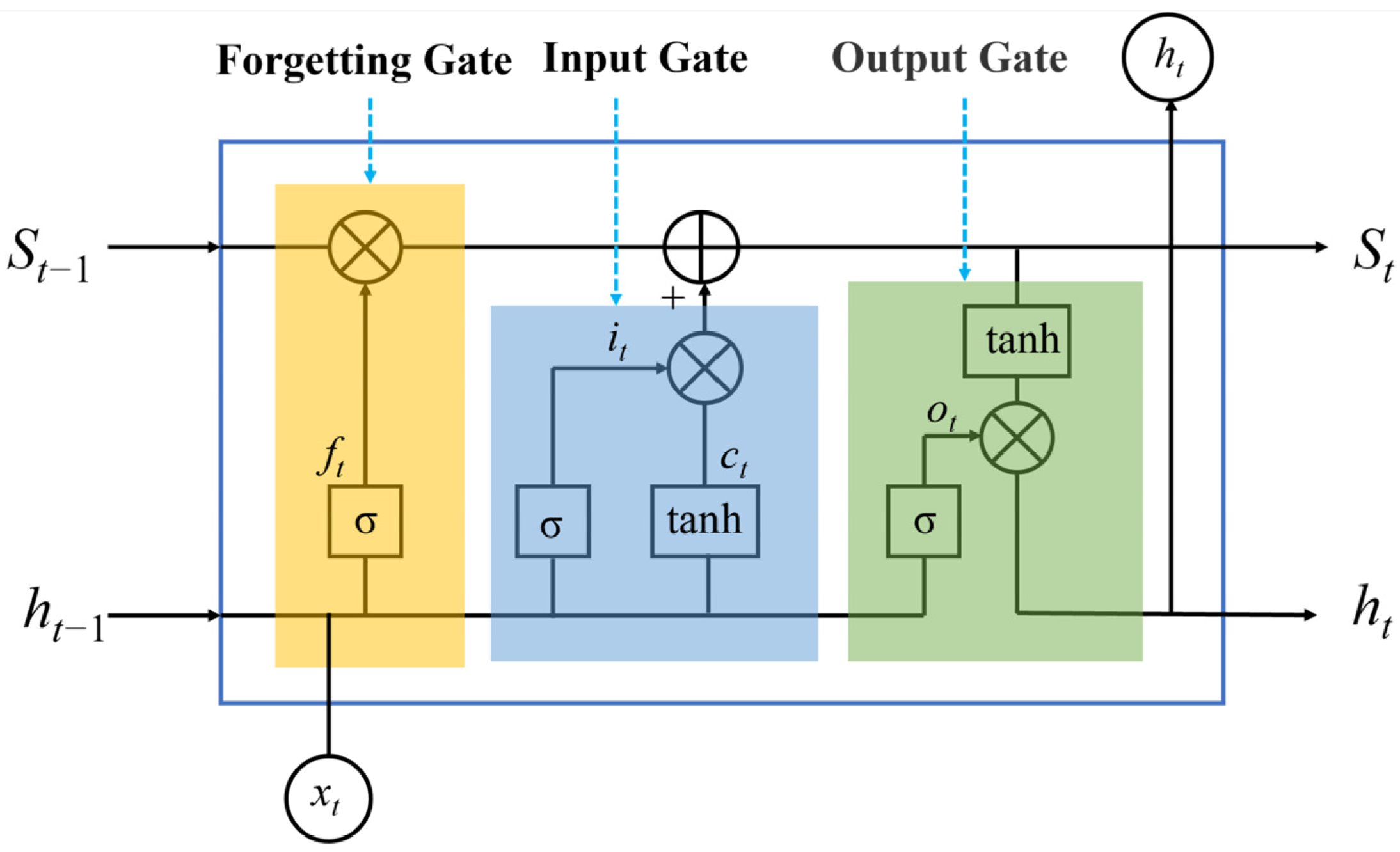
25], etc., have all been used for wind power forecasting. Among them, LSTM is a recurrent version of deep learning, which applies many temporal latent layers to effectively learn the strong temporal feature of wind power data [26], realizing the full utilization of long-distance time series information. However, LSTM only contains one-way information and the time correlation between data is not considered comprehensively. Therefore, the bidirectional long short-term memory neural network (BiLSTM), combining two groups of LSTMs with opposite directions, has emerged, which contains both historical and future information, and this network has been shown to improve the prediction accuracy [5]. Therefore, this paper conducts power forecasting based on BiLSTM.
The single model has limitations [27], so the hybrid model emerges as the times require, giving full play to the advantages of each model to achieve the goal of complementarity. It mainly includes two combination methods. One is an overall combination based on model performance. By assigning different weights, the prediction results of multiple single models are linearly combined to further improve the prediction accuracy. For example, [28] combines four neural networks: BP, Elman, ELM, and generalized regression neural network (GRNN); [29] combines three deep neural networks: LSTM, DBN, and echo state network (ESN). However, there are too many selection methods for the basic single models and their corresponding weights, and it is difficult to determine whether the performance of multiple single models is complementary, resulting in excessive randomness of the results. The other is component forecasting based on data features, extracting similar data through feature engineering, to enhance the representativeness and adaptability of the model to specific situations through the refinement of data selection [
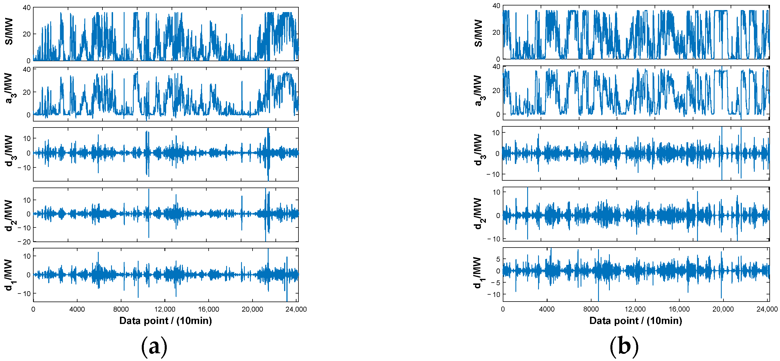
30]. The following methods are currently popular: the original data is denoised by wavelet decomposition [31], empirical mode decomposition (EMD) [32], ensemble empirical mode decomposition (EEMD) [33], variational modal decomposition (VMD) [34], etc., to be decomposed into components of different frequency bands, and appropriate models are used to predict each subsequence separately. Based on different features (such as weather conditions, wind conditions, output mode, power change trend, etc.), cluster analysis is carried out on the original data [35,36], and power forecasting is made for different types of data, respectively; a similarity calculation method is defined in units of days, and the similar day data are extracted for model training and forecasting [37]. However, the above methods mostly extract feature similarity from the perspective of power output—ignoring the wind speed and wind direction, which are the two meteorological factors that have the greatest impact on future power—and have not excavated the strong correlation between the above two factors and power. Therefore, based on emphasizing the inseparable relationship between the above two factors and power, this paper focuses on extracting similar data from these two perspectives for component forecasting.
Table 1 shows the comparison of the above models. In addition to the above models, data pre-processing and post-processing are also effective ways to improve the accuracy of wind power forecasting. The pre-processing of the data mainly uses a maximum information coefficient (MIC) [26], principal component analysis (PCA) [17], conditional mutual information [38], etc., to perform correlation sorting, and to reduce the dimension of high-dimensional input features. By introducing as many features as possible, the forecasting model can reflect the impact of complex external conditions on wind power to some extent. However, the features with lower correlation have limited improvement on prediction performance. Traditional methods do not consider the different influence of the input features on the change of wind power in different wind farms, that is, different wind farms are applicable to different model input features. At the same time, when multiple original features are used as the input features of the prediction model, the complexity of the model will be increased, and the running speed of the model will be seriously reduced. In order to improve the above situations, it is necessary to have the corresponding algorithm to select several appropriate features from multiple original features as the input variables of the model. The relevant feature selection algorithm can not only screen out the features that have a greater impact on wind power and eliminate the coupling relationship between variables, but also help to improve the running speed of the model, which makes the prediction model achieve higher prediction accuracy and efficiency with less input. The post-processing of data is mainly to correct the error of the predicted wind power [39] by describing the distribution of the prediction error, ref. [40] by predicting the error, and to correct the preliminary prediction power value. Compared with the load forecast, due to the uncertainty of wind speed, the wind power forecasting result is more volatile and there is still a large error in the preliminary forecasting. The preliminary prediction result is substituted into the error model, and the error value obtained is correspondingly superimposed with the preliminary forecasting value as the prediction correction result, which plays the role of checking the leakage and filling it. At the same time, different types of models are selected for the preliminary forecasting and error correction, which can avoid the limitations of a single model to a certain extent and give full play to the advantages of different models to further improve the prediction accuracy. The error correction has strong generality and is not limited to the specific forecasting process. Therefore, the multi-link forecasting method of “ input screening + model combination + error correction” has become a research hotspot and strives to maximize the prediction accuracy from the perspective of each link optimization.
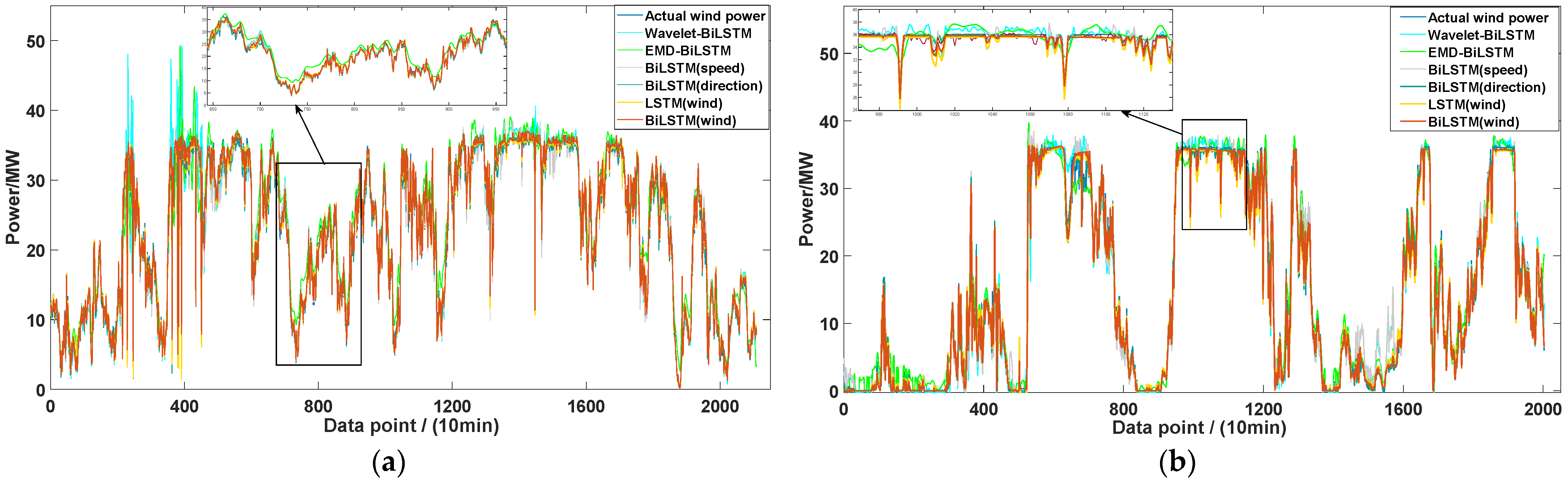
In summary, this paper proposes a short-term wind power forecasting method based on feature analysis and error correction. First, the MIC is introduced to analyze the correlation of multiple factors affecting wind power, and then feature selection is performed based on this. Second, the data are divided based on wind speed, and cluster analysis is conducted on the data from the aspect of wind direction. Then, each component builds a prediction model based on the BiLSTM to complete the preliminary forecasting of wind power. Finally, lightGBM is used to perform error forecasting and correct the preliminary prediction results. The results of practical examples show that the method proposed in this paper effectively improves the forecasting accuracy and establishes a hybrid forecasting framework including feature selection, similar data component extraction, model forecasting, and error correction. Our contributions are summarized as follows:
  • MIC is used for feature selection. Several factors with the strongest correlation with wind power are selected from multiple features, which avoids the interference of irrelevant features on the wind power prediction results, reduces the input features dimension, reduces the workload of neural network, and thus greatly improves the operation speed. In addition, the features most closely related to power can also be observed, thus laying a foundation for the extraction of similarity components.
  • A hybrid model based on component forecasting is used for wind power forecasting. The strong correlations between wind speed and power, wind direction and power are separately mined. The prediction components are extracted from the above two features for the first time, which makes the similarity between components stronger. The relationship between wind turbine output and wind speed is fully utilized, and the influence of wind blowing from different wind directions on wind energy absorbed by wind turbines is considered. This provides a new idea for improving the accuracy of wind power forecasting, which has not been studied in the previous literature.
  • Based on the forecasting model, an error correction method is proposed. Since the correlation between prediction error and input features such as wind speed and wind direction are smaller than the correlation between predicted power and the above factors, the data post-processing method uses the lightGBM algorithm to predict the error for the first time, which is more suitable for processing data with low correlation. At the same time, it can make up for the shortcomings caused by only using the BiLSTM model. The two algorithms with completely different principles complement each other, making the prediction results more accurate.
The rest of this paper is organized as follows: The basic principles and methods of MIC feature selection and the extraction of similar data components based on wind speed and wind direction are introduced in Section 2. The forecasting model and error correction model are established in Section 3. The example analysis is in Section 4. Finally, conclusions are drawn in Section 5.

2. Feature Analysis and Extraction

2.1. Correlation Analysis Based on MIC

The MIC was proposed in 2011 to measure the degree of correlation between variables [41]. Table 2 compares various correlation analysis methods. Traditional correlation analysis methods, such as linear fitting and Pearson et al., can only analyze the correlation between linear data, and Spearman can analyze the simple and monotonous nonlinear correlation on this basis. Therefore, their scope of application is small. Moreover, these methods have poor robustness. PCA and its improved algorithm kernel principal component analysis (KPCA) are two popular correlation analysis methods at present which enhance the ability of data processing. However, the former has difficulty dealing with data sets that are not linearly separable, and the latter is too dependent on the selection of kernel function parameters. MIC can not only describe linear and nonlinear (such as periodicity and sinusoidal) relations between variables but also tap the potential non-functional relations [42]. Moreover, it shows good robustness to data containing noise, such as wind speed and wind power, and has low computational complexity.
The basic principle of MIC is as follows: if there is correlation between two variables, the scatter diagram formed by them is drawn, and the corresponding mutual information (MI) value is calculated and regularized under different grid division methods, wherein the maximum MI value is the MIC of the two variables.
MIC is used to analyze the correlation between different features and wind power as follows:
(1) Calculate the MI. Assume that the feature is X = x i ( i = 1 , 2 , , N ) ; the wind power is Y = y i ( i = 1 , 2 , , N ) ; N is the sample number. The MI value between X and Y is:
I M I ( X , Y ) = x X y Y ( p ( x , y ) log 2 p ( x , y ) p ( x ) p ( y )
where, p ( x , y ) is the joint probability density between X and Y ; p ( x ) and p ( y ) are the marginal probability density of X and Y , respectively.
(2) Divide the grid. D = ( x i , y i ( i = 1 , 2 , , N ) is a binary data set composed of two variables. A scatter plot is formed, and the current two-dimensional space is divided into a grid of m × n , denoted as G ( m , n ) . There are various ways to divide the grid of m × n , so the MI value calculated is different, and the largest MI value is selected:
I M I max ( D , m , n ) = max I M I ( D G )
(3) Normalization. Normalized the maximum MI values under different grids:
M ( D ) m , n = I M I max ( D , m , n ) log 2 min ( m , n )
(4) Calculate the MIC. The MIC is:
I M I C ( D ) = max m n < B ( N ) M ( D ) x , y
where, B ( N ) is the upper limit of grid division and will usually be selected as B ( N ) = N 0.6 .
MIC values range from 0 to 1. The larger the MIC value is, the stronger the correlation is. Therefore, the features strongly correlated with wind power are selected as model input features.

2.2. Feature Analysis of Wind Speed

2.2.1. Relationship between Wind Speed and Wind Power

In short-term wind power forecasting, wind speed is the leading factor determining the output power of wind farms, which is an essential parameter for the energy system operation [43]. The randomness and uncertainty of wind speed make wind power have the same characteristics, so full analysis of wind speed can greatly reduce the wind power forecasting error. Therefore, wind speed is selected as the primary feature representative of power forecasting. As the biggest factor affecting wind power, there is a strong correlation between them. Figure 1 shows the relationship between wind speed and wind turbine output. The theoretical relationship between them is as follows:
P v = 0 0 < v < v i n , v > v o u t 1 2 C P ρ A v 3 v i n v <   v r P r v r v < v o u t
where, P(v) is the theoretical output of wind turbine, kW; P r is the rated power, kW; v is the real-time wind speed, m/s; v i n , v r , and v o u t are the cut-in wind speed, rated wind speed, and cut-out wind speed, respectively, m/s; C P is the wind energy utilization coefficient; ρ is the air density, kg/m3; A is the swept area by the wind wheel, m2.
NWP is the main source of wind speed forecasting data. Based on the above analysis, the data are divided according to NWP wind speed to improve the correlation. The partition nodes are cut-in wind speed, rated wind speed, and cut-out wind speed. Therefore, the raw data are divided into three categories: 0 v < v i n or v v o u t is the zero-power group; v i n v <   v r is the standard-power group; v r v < v o u t is the rated-power group.
Due to the existence of certain errors in NWP wind speed data, in order to improve accuracy, this paper further divides the wind speed according to the distribution law and considering the wind speed fluctuation. The change trend of wind speed in a certain period is analyzed in order to reserve a certain margin at each partition node and reduce the error. The wind speed fluctuation is depicted as follows:
C t = sign v t 2 T v t 3 T + sign v t T v t 2 T + sign v t v t T
sign x = 1 x > 0 0 x = 0 1 x < 0
where, v t is the NWP wind speed at time t; T is the time resolution; v t 3 T , v t 2 T , and v t T represent the NWP wind speed at 3T minutes, 2T minutes, and T minutes before time t, respectively; C t describes the changing trend of wind speed at time t, when C t > 0 , indicates that wind speed shows an upward trend, and the partition nodes can be appropriately reduced; when C t < 0 , indicates that the wind speed decreases, and the partition nodes can be appropriately improved.

2.2.2. Wind Speed Probability Distribution Model

Wind speed generally conforms to the two-parameter Weibull distribution, and the cumulative distribution function is as follows:
F v V = 1 exp V c k
The probability density function is:
f v = k c v c k 1 exp v c k
where, v is the wind speed, m/s; V is the given wind speed, m/s; k is the shape parameter; c is the scale parameter.
When a local wind condition has multi-peak characteristics, it can be fitted with a mixed Weibull. The mixed Weibull belongs to a weighted model, which is composed of multiple Weibull based on weights. The cumulative distribution function is as follows:
F n v V = i = 1 n ω i 1 exp V c i k i
i = 1 n ω i = 1
where, n is the number of Weibull; ω i is the weight of the ith Weibull; k i is the shape parameter of the ith Weibull; c i is the scale parameter of the ith Weibull.
The probability density function is:
f n v = i = 1 n ω i k i c i v c i k i 1 exp v c i k i
Maximum likelihood estimation is a commonly used method with high accuracy in Weibull fitting [44]. This paper performs Weibull fitting on the wind speed of the wind farm. According to the contents of the previous section, when wind speed shows an upward trend, on the cumulative distribution curve of wind speed, each partition node becomes the corresponding wind speed when the probability of the current cumulative distribution decreases by 2%, denoted as v i n u p , v r u p , and v o u t u p , respectively; when the wind speed shows a downward trend, each partition node becomes the corresponding wind speed when the current cumulative distribution probability increases by 2%, denoted as v i n d o w n , v r d o w n , and v o u t d o w n , respectively. The specific situation is shown in Figure 2:

2.3. Feature Analysis of Wind Direction

In order to obtain more abundant wind resources, maximize the capture of wind energy, and reduce the influence of tower shadow effect, wind farms generally adopt the strategy of deploying upwind wind turbines in the prevailing wind direction [45]. As a result, wind turbines have different abilities to capture wind blowing from different directions. This is because, although wind turbines are generally equipped with a yaw system, there is a delay effect in the control process and, due to the different wind paths, the ground roughness and obstacles are different, resulting in different wind speeds reaching the wind turbine. Therefore, wind direction is also one of the important features affecting wind power and must be considered in power forecasting.
Clustering can group data points into different clusters based on their similarity or density, automatically extracting intra-class similarities as well as inter-class differences [46]. In general, the analysis of wind direction is performed mostly by drawing a wind direction rose chart. This meteorological tool can intuitively describe the wind direction characteristics of a certain area. The polar coordinates of the wind rose chart are generally divided into 4, 8, or 16 wind directions. At the same time, considering that with the increase in the number of clusters the calculation is more complex, but the improvement of the clustering performance is limited, the Elbow’s method is generally used to determine the optimal number of clusters [47]. The Elbow’s method selects the optimal number of clusters by calculating the Sum of Squared Error (SSE) under different cluster number K. As K continues to increase, SSE will gradually decrease. During the change of SSE, there will be an inflection point, called “elbow” point, at which the decline rate suddenly slows down, and the corresponding K value is considered as the optimal number of clusters. We drew inspiration from the wind direction division rules of the wind rose chart and combined it with the Elbow’s method to determine the cluster number to be 4. Therefore, only four directions subsets are involved in this paper. Cluster analysis method is used to divide the standard-power group data into four categories from the aspect of wind direction: north, east, south, and west. Since the data of the zero-power group and the rated-power group are less, and their power is mostly fixed at 0 or the rated power, the correlation between power and wind speed is much greater than that between power and wind direction, so only the wind direction clustering is performed on the data of the standard-power group. In addition, due to the large amount of data, the k-means clustering algorithm, which is most typical, is selected for cluster analysis.
The initial clustering center of k-means algorithm needs to be selected randomly or manually, and the quality of the initial clustering center greatly affects the clustering result. In order to ensure the accuracy of clustering, in this paper, the data of due north (348.75°–11.25°), due east (78.75°–101.25°), due south (168.75°–191.25°), and due west (258.75°–281.25°) are firstly selected. The fuzzy c-means algorithm (FCM), which is more suitable for processing less data, is used to select the clustering centers of the above data in four directions as the initial clustering centers of k-means to ensure that the clustering results contain wind direction information.

3. Forecasting Model Considering Error Correction

3.1. BiLSTM Model

The LSTM neural network constructs a larger deep neural network through complex nonlinear units, which can reflect the long-term memory effect and thus carry out deep learning. It is a special network in the recurrent neural network (RNN) [48]. At each time compensation, combined with the output of the last point, content selection is realized through the gate structure [49]. LSTM has three layers, and its basic network unit is shown in Figure 3. The basic unit contains input gate, forget gate, and output gate. x t is the input of the current layer; h t 1 is the output of the previous layer. After they pass through the forget gate together, they output any value between 0 and 1 to the old cell state S t 1 to decide the forgotten part. “0” means “forget all”; “1” means “pass all”. The x t in the input gate goes through the sigmoid and tanh functions, respectively, and the obtained results are multiplied to generate new information. Then, the new information plus the forgotten S t 1 , and their sum, is the new cell state S t . After S t passes through the tanh function, it determines the output together with o t . The calculation formulas are as follows:
f t = σ ( ω x f x t + ω h f h t 1 + b f )
i t = σ ( ω x i x t + ω h i h t 1 + b i )
c t = σ ( ω x c x t + ω h c h t 1 + b c )
o t = σ ( ω x o x t + ω h o h t 1 + b o )
S t = c t × i t + S t 1 × f t
h t = o t × tanh ( S t )
where, σ is the sigmoid function; ω x f , ω x i , ω x c , and ω x o are the weight matrix of x t with forgetting gate, input gate, primitive input, and output gate, respectively; ω h f , ω h i , ω h c , and ω h o are the weight matrix of h t 1 with forgetting gate, input gate, primitive input, and output gate, respectively; b f , b i , b c , and b o are the bias vectors of the corresponding parts.
Wind power is a time series with strong temporal correlation. The wind power at a certain time is not only related to multiple NWP meteorological features, but also related to the historical or future wind power at an adjacent time or at the same time of different days. The temporal correlation characteristic of wind power mainly comes from several NWP meteorological features with strong correlation with it, such as wind speed and wind direction, whose influence on power is enough to cover the influence of most other NWP features. Taking NWP wind speed as an example, under normal circumstances, there is time series autocorrelation between the current wind speed and the historical or future wind speed at an adjacent time or at the same time of different days, so it shows a certain degree of temporal correlation characteristic.
LSTM has a certain memory function for historical data, that is, when forecasting the wind power P ^ ( t ) at time t, LSTM not only considers the influence of the input features at time t on the wind power prediction value P ^ ( t ) but also considers the influence of the prediction power P ^ ( t 1 ) at time t − 1. The same is true of predictions at other times. Therefore, in the wind power forecasting at time t, not only the current time information is used but also the long-distance historical information is used. However, it can only use the past information and transmit from front to back, which has limitations. BiLSTM solves these problems by using two positive and negative LSTMs. Based on these LSTMs, it also considers the influence of the prediction power P ^ ( t + 1 ) at the time t + 1 on P ^ ( t ) , which enables it to capture both historical and future information. In addition, the possible phase lag problem in one-way prediction is solved by it. Therefore, BiLSTM is more suitable for time series prediction, and shows better performance in the field of forecasting. Its output expression is:
h t = concat ( h t f , h t b )
where, h t f and h t b are the forward and backward LSTM output vectors, respectively; concat is representing the splicing operation.
The BiLSTM network structure is shown in Figure 4.

3.2. LightGBM Model

LightGBM is a framework for the implementation of the GBDT algorithm, which is an improvement on the XGBoost algorithm. It has obvious improvement in performance, efficiency and running speed [50]. LightGBM is one of the algorithms with excellent performance at present.
Compared with the traditional XGBoost algorithm, LightGBM mainly obtains more accurate information gain through the gradient-based one-sided sampling strategy (GOSS) and realizes feature dimensionality reduction by combining high-dimensional features through the mutually exclusive feature compression strategy (EFB), thereby reducing computational complexity and improving efficiency. In addition, the optimization also involves the following aspects: the decision tree algorithm based on Histogram reduces memory usage; the Leaf-wise growth strategy with depth limit deepens the decision tree; direct support for category features; cache hit rate optimization; histogram-based sparse feature optimization; multi-threading optimization; etc.

3.3. Establishment of Forecasting Model

BiLSTM has good processing performance for data with strong correlations, while the LightGBM algorithm is more suitable for processing data with weak correlations. Therefore, in this paper, BiLSTM is used to establish the nonlinear relationship between multi-dimensional features and wind power and to predict the wind power needed to obtain the preliminary predicted power. The LightGBM algorithm is used to forecast the error in order to correct the preliminary predicted power. The calculation method is as follows:
Historical data prediction error:
e ( t n T ) = P ^ ( t n T ) P ( t n T ) , n = 1 , 2 , , N
where, e ( t n T ) , P ^ ( t n T ) , and P ( t n T ) are, respectively, power prediction error, power forecasting value, and actual power at time ( t n T ) , MW; T is the time resolution; N is the historical data capacity.
e ^ ( t ) = f X ( t )
where, X ( t ) is the input feature at time t , including weather features, preliminary predicted power, historical error data, etc. f ( ) is the nonlinear relationship between the input features and the error prediction value.
Therefore, the revised power prediction value is:
P ^ ( t ) = P ^ ( t ) e ^ ( t )
The overall process of this paper is shown in Figure 5. The specific steps are as follows:
(1)
Feature selection. The MIC value between multi-dimensional features and wind power is calculated, and the features with strong correlation are selected as input features.
(2)
Wind speed division. Calculate the fluctuation type of the wind speed of the original data, find the partition nodes based on the cut-in wind speed, rated wind speed, and cut-out wind speed, and divide the original data.
(3)
Wind direction clustering. FCM is used to select the clustering centers of the data with the wind directions of due north, due east, due south, and due west, respectively, as the initial clustering centers of the k-means algorithm. Then, k-means is used to cluster the data of the standard-power group into four categories of north, east, south, and west.
(4)
Power forecasting. For each type of data, a BiLSTM forecasting model is constructed to predict wind power, and the preliminary prediction results are sorted according to the time sequence.
(5)
Error correction. The LightGBM model is applied for error forecasting to correct the preliminary power forecasting results.

4. Case Study

This paper takes a wind farm (wind farm A) in Northwestern China and a wind farm (wind farm B) in North China as the research objects. The installed capacity of both wind farms is 45 MW. The data of the two wind farms from 1 May to 15 August 2018 are selected as relevant experimental samples, including the actual wind power data and a variety of historical mesoscale NWP meteorological data. The meteorological features include wind speed, wind direction, temperature, pressure, and humidity. The time resolution T = 10   min , and the data deviating from the actual situation are excluded. Among them, the average wind speed of wind farm A was relatively large, with relatively strong fluctuations; the average wind speed of wind farm B was relatively small, with relatively weak fluctuations. The data from a total of 92 days from May to July were selected as a training set, and data from the remaining 15 days were used as a testing set.

4.1. Feature Processing

4.1.1. MIC Feature Selection

The items listed in Table 3 are the alternatives for the input features. In order to select the optimal feature, the MIC value between features and the actual wind power were calculated, respectively, and several items with strong correlations were selected as the input features. The higher the MIC value, the stronger the correlation between its corresponding features and wind power. From Table 3, we observe that for wind farm A, among various NWP meteorological features, the MIC value between wind speed and actual wind power was the highest, followed by wind direction, temperature, pressure, and humidity, in turn. Three meteorological features with the strongest correlation were selected as input features for wind farm A, namely wind speed, wind direction, and temperature. For wind farm B, among various NWP meteorological features, the MIC value between wind speed and wind power was also the highest, followed by temperature, wind direction, pressure, and humidity, in turn. Three meteorological features with the strongest correlation were selected as input features for wind farm B, which were also wind speed, wind direction, and temperature. In addition, we also analyzed the correlation between the historical wind power data and the wind power at the current time. From the MIC value, we observed that there was a strong correlation between them, and the MIC value of the historical wind power was higher when it was closer to the forecast time. Therefore, we also considered historical wind power data as an input feature. Due to the limitation of time scale, when the time scale was 24 h, we additionally selected the wind power from the previous 24 h as the input feature; when the time scale was 12 h, we additionally select the wind power from the previous 12 h as the input feature; when the time scale was 8 h, we additionally select the wind power from the previous 8 h as the input feature. Figure 6 shows the wind power forecasting when the time scale is T . When the prediction time scale T = 24   h , after the training set was used to complete the model training, the 144 test samples of every 24 h (1 day) scale were selected to forecast the power through the trained network. The input time series were the NWP wind speed, wind direction and temperature every 10 min in the next 24 h, as well as the actual wind power series in the first 24 h of the corresponding test sample points. The output time series was the wind power prediction value every 10 min in the next 24 h, and the experimental content was repeated until the 15-day prediction task was completed.

4.1.2. Wind Speed Division Results

Figure 7 shows wind speed frequency histograms of two wind farms. The wind speed in wind farm A is bimodal distribution, so the mixed Weibull fitting composed of two Weibull distributions was used; the wind speed in wind farm B is unimodal distribution, so the single Weibull fitting was used. It can be intuitively seen that the wind speed distribution of wind farm A is relatively scattered, and the wind speed frequency of 3–8 m/s is similar; the wind speed distribution of wind farm B is relatively concentrated, and the wind speed frequency of 6–8 m/s is relatively high. Figure 8 shows the Weibull fitting results, where c 1 = 2.946 , c 2 = 5.721 , k 1 = 2.295 , k 2 = 2.632 , ω 1 = 0.208 , and ω 2 = 0.792 in wind farm A; scale parameter c = 2.165 , shape parameter k = 9.156 in wind farm B. According to the actual situation of the wind farm, v i n = 3   m / s , v r = 13   m / s and v o u t = 25   m / s . Since none of the selected historical data exceeds the cut-out wind speed, only the cut-in wind speed and the rated wind speed were considered when dividing the wind speed. Figure 9 shows the fitted wind speed cumulative distribution function. According to the rules in Figure 2, v i n , A u p = 2.808   m / s , v r , A u p = 12.149   m / s , v i n , A d o w n = 3.192   m / s , and v r , A d o w n = 14.740   m / s in, wind farm A can be obtained; v i n , B u p = 2.639   m / s , v r , B u p = 12.551   m / s , v i n , B d o w n = 3.323   m / s , and v r , B d o w n = 13.510   m / s in wind farm B. In wind farm A, when wind speed fluctuation shows an upward trend, 0 v < 2.808   m / s is the zero-power group, 2.808   m / s v < 12.149   m / s is the standard-power group, and v 12.149   m / s is the rated-power group; when wind speed fluctuation shows a downward trend, 0 v < 3.192   m / s is the zero-power group, 3.192   m / s v < 14.740   m / s is the standard-power group, and v 14.740   m / s is the rated-power group. In wind farm B, when wind speed fluctuation shows an upward trend, 0 v < 2.639   m / s is the zero-power group, 2.639   m / s v < 12.551   m / s is the standard-power group, and v 12.551   m / s is the rated-power group; when wind speed fluctuation shows a downward trend, 0 v < 3.323   m / s is the zero-power group, 3.323   m / s v < 13.510   m / s is the standard-power group, and v 13.510   m / s is the rated-power group.

4.1.3. Wind Direction Clustering Results

Figure 10 shows the changes of SSE with the value of K after the clustering of wind direction data of the two wind farms. When K = 4 for wind farm A and K = 3 for wind farm B, the SSE is greatly reduced, which represents that the distortion degree is greatly reduced and then slowly decreases. Combined with the drawing rules of the wind direction rose chart, the number of clusters is selected as 4.
The data with the NWP wind directions of due north, due east, due south, and due west were selected, and the cluster centers of the data in each direction above were clustered by FCM. The results are shown in Table 4. The above four points were used as the initial clustering center of k-means. Through the k-means algorithm, all the data of standard-power group were clustered into four subsets of east, west, north, and south according to the wind direction. Figure 11 and Figure 12 show the three-dimensional relationship between wind direction sine, wind direction cosine, and power before and after clustering, respectively.

4.2. Data Normalization

The original data are normalized as follows:
x n = x x min x max x min
The predicted power is reversely normalized as follows:
x = x n ( x max x min ) + x min
where, x n is the normalized data; x is the actual value; x min and x max are the minimum value and maximum value of each type of data, respectively.

4.3. Evaluation Index of Forecasting Effect

The fitting degree between the predicted power and the actual power is the criterion for evaluating the goodness of the forecasting model. In this paper, the mean absolute error (MAE), root mean square error (RMSE), and mean relative error (MAPE) of the results are calculated as follows:
M A E = 1 n c i y i
R M S E = 1 n i = 1 n c i y i 2
M A P E = 1 n × i = 1 n c i y i y i × 100 %
where, c i and y i are predicted value and true value, respectively; n is the sample size.

4.4. Analysis of Wind Power Forecasting Results

In order to verify the effectiveness of the proposed method, this paper conducts the following three rounds of forecasting. The time scale of the first and second rounds of forecasting is 24 h, and the time scale of the third round of forecasting includes 24 h, 12 h, and 8 h.

4.4.1. Basic Single Model Forecasting

In order to verify the accuracy of the basic model adopted in this paper, first, the single BP, RBF, Elman, LightGBM, LSTM, and BiLSTM neural networks models were used to predict the unclassified original data. For the BP neural network, the maximum iteration number is 200, the number of hidden layer nodes is 5, the learning rate is 0.1, and the learning objective is 0.00004. For the RBF neural network, the spread is 20, and the number of neurons is 10. For the Elman neural network, the hidden layer has 11 neurons, and the maximum iteration number is 2000. The parameters of LSTM are shown in Table 5. The parameters of unidirectional LSTM in BiLSTM are the same as those of LSTM. Table 6 shows the forecasting results of the above models, and Figure 13 shows the comparison of the results of the above models. Table 7 shows the prediction results of a single BiLSTM for wind farm A when the parameters of LSTM are changed, from which we can know that the accuracy is higher under the parameters selected in the Table 5.
Combined with Figure 7 and Figure 13, we observe that the wind speed of wind farm A changed frequently due to the relatively scattered distribution of wind speed, and then showed the characteristics of relatively large fluctuation in power generation; wind farm B had a relatively concentrated wind speed distribution, which resulted in less frequent changes in wind speed, and then showed a low fluctuation in power generation. From Figure 13, we observe that BiLSTM had the best prediction performance among the six basic models, followed by LSTM. For wind farm A, compared with RBF model with a large error, the MAE, RMSE, and MAPE of BiLSTM were reduced by 0.9141 MW, 1.1711 MW, and 12.180%, respectively; when compared with LightGBM, the MAE, RMSE, and MAPE of BiLSTM were reduced by 0.0891 MW, 0.7785 MW, and 6.585%, respectively; and when compared with LSTM with better forecasting results, the MAE, RMSE, and MAPE of BiLSTM were reduced by 0.1026 MW, 0.4238 MW, and 3.985%, respectively. For wind farm B, compared with RBF model with a large error, the MAE, RMSE, and MAPE of BiLSTM were reduced by 0.6417 MW, 1.1023 MW, and 22.430%, respectively; when compared with LightGBM, the MAE, RMSE, and MAPE of BiLSTM were reduced by 0.2361 MW, 0.7805 MW, and 10.436%, respectively; and when compared with LSTM with better forecasting results, the MAE, RMSE, and MAPE of BiLSTM were reduced by 0.1738 MW, 0.0075 MW, and 4.789%, respectively. From the above analysis, we know that the MAE, RMSE, and MAPE of BiLSTM are all the lowest, which shows that the prediction accuracy of the BiLSTM was better than that of the five other basic models. From Figure 13, we can also observe that the prediction curve obtained by BiLSTM was most like the actual wind power curve with a high degree of overlap, which verifies the superiority of the BiLSTM model. Although BiLSTM performed best in these six basic models, the overall prediction accuracy still cannot meet the high requirements of practical application. Therefore, it is necessary to improve the prediction performance through the following two rounds of method improvement. This is because, although the basic model has universality and is widely used in load forecasting, wind power forecasting, photovoltaic forecasting, and other forecasting fields, compared with load and photovoltaic power, which have strong daily variation regularity, wind power has extremely strong uncertainty. The basic model has a poor ability to capture this uncertainty and has a certain delay effect. Especially at points with high wind power fluctuations, such as the peak and valley of the curve, the basic model is likely to overlook the changes of these mutation points, which makes the prediction performance poor. Extracting the characteristics of wind through feature engineering and constructing a more suitable prediction model for wind power can improve this situation. Therefore, we combined feature engineering with the basic model in the second round of forecasting. In addition, the single basic prediction model has poor generalization ability for different data and cannot fully include various factors, resulting in its inability to achieve high-precision prediction in certain specific application scenarios. Wind power is influenced by multiple factors, so the single basic model is difficult to fully learn, which will lead to unsatisfactory prediction results. Especially in the case of extreme weather or large changes in meteorological factors, the prediction will show significant deviation. The peak or valley of the wind power curve mostly corresponds to the occurrence of large changes of wind speed, so the single basic model has poor performance on the peak or valley of the power curve. The hybrid prediction method considers the respective advantages of different models simultaneously, which can effectively overcome the inherent limitations of the single prediction model and significantly improve the accuracy of prediction. Therefore, we added the LightGBM correction model to form a hybrid prediction model in the third round of forecasting.

4.4.2. Forecasting after Similar Data Component Extraction

In order to verify the effectiveness of the feature analysis method used in this paper, the method in this paper is compared with many other methods to verify the prediction effect of using different similarity data extraction methods for forecasting based on the same basic model. This round included six forecasting models. After wavelet decomposition of the original data, BiLSTM model power forecasting was performed for each group, which is denoted as Wavelet-BiLSTM; after EMD decomposition of the original data, BiLSTM model power forecasting was performed for each group, which is denoted as EMD-BiLSTM. Only considering wind speed division, data were divided into three groups: zero-power group, standard-power group, and rated-power group, and each group was forecasted by BiLSTM, denoted as BiLSTM (speed). Only considering wind direction clustering, data were divided into four groups: north group, east group, south group, and west group, and each group was forecasted by BiLSTM, denoted as BiLSTM (direction). Considering both wind speed division and wind direction clustering, the 6 groups of data after classification were, respectively, forecasted by LSTM and BiLSTM, denoted as LSTM (wind), and BiLSTM (wind). The wavelet decomposition and EMD decomposition results are in Figure 14 and Figure 15. In Figure 15, the original data of wind farm A were decomposed into 10 IMFs (the blue lines) and a residual component (the red line) through EMD; the original data of wind farm B were decomposed into 9 IMFs (the blue lines) and a residual component (the red line) through EMD.
Table 8 shows the forecasting results of the above models. Figure 16 shows the forecasting results of the two wind farms. Due to the use of spline interpolation for classification and screening in EMD, the shortcomings of separation and intermittency restricted the effectiveness of similar frequency components separation. Moreover, it was susceptible to noise interference, resulting in mode mixing and endpoint effects [51]. A large amount of wind power data inevitably contains noise, so EMD-BiLSTM performed the worst. At the same time, due to the excessive EMD components, the prediction time and calculation cost of the prediction model were greatly increased. We observed that BiLSTM (wind) had the best prediction performance among the six hybrid models. For wind farm A, compared with the BiLSTM model, the MAE, RMSE, and MAPE of BiLSTM (wind) were reduced by 0.5544 MW, 1.6256 MW, and 22.543%, respectively; when compared with BiLSTM (speed), the MAE, RMSE, and MAPE of BiLSTM (wind) were reduced by 0.4008 MW, 1.1404 MW, and 11.2261%, respectively; and when compared with BiLSTM (direction), the MAE, RMSE, and MAPE of BiLSTM (wind) were reduced by 0.0882 MW, 0.2903 MW, and 4.7308%, respectively. For wind farm B, compared with the BiLSTM model, the MAE, RMSE, and MAPE of BiLSTM (wind) were reduced by 0.7749 MW, 1.0830 MW, and 13.642%, respectively; when compared with BiLSTM (speed), the MAE, RMSE, and MAPE of BiLSTM (wind) were reduced by 0.4562 MW, 0.6644 MW, and 12.4738%, respectively; and when compared with BiLSTM (direction), the MAE, RMSE, and MAPE of BiLSTM (wind) were reduced by 0.0294 MW, 0.4316 MW, and 4.5341%, respectively. From the above analysis, we know that the MAE, RMSE, and MAPE of BiLSTM (wind) are lower than that of all forecasting methods in the previous round, and the accuracy of the methods proposed in this round has been greatly improved. The prediction curve had a high fitting degree with the actual power curve. The prediction effect of BiLSTM (wind) was better than that of Wavelet-BiLSTM and EMD-BiLSTM, which verifies the effectiveness of the similarity data extraction method proposed in this paper. At the same time, it was also better than that of BiLSTM (speed) and BiLSTM (direction), which were better than BiLSTM, indicating that both wind speed division and wind direction clustering play a positive role in improving the prediction accuracy, and the hybrid forecasting model of both of them strengthens this positive effect.

4.4.3. Error Correction of Forecasting Results

In order to eliminate the time dependence, this round verified the model effect by changing the time scale and carried out experiments with time scales of 24 h, 12 h, and 8 h, respectively. At the same time, in this round, LightGBM was used to correct the prediction results of BiLSTM (wind), denoted as BiLSTM-LightGBM. The MIC correlation analysis between various features and preliminary prediction error is shown in Table 9. We observed that for wind farm A, under the three different time scales, the MIC value between the BiLSTM (wind) forecasting power and the prediction error was the highest, followed by wind speed, power prediction error from the previous 10 mins and the previous 20 mins, in turn. Other features were relatively weakly correlated with prediction error. The four features with the strongest correlation were selected as the input features for wind farm A, namely BiLSTM (wind) forecasting power, wind speed, power prediction error from the previous 10 mins and 20 mins. For wind farm B, under the three different time scales, the MIC value between the BiLSTM (wind) forecasting power and the prediction error was also the highest, followed by the power prediction error from the previous 10 mins, wind speed, and the power prediction error from the previous 20 mins, in turn. Other features are relatively weakly correlated with prediction error. The four features with the strongest correlation were selected as the input features for wind farm B, which were the same as wind farm A.
The error value was forecasted by LightGBM, so all preliminary power prediction results could be corrected 10 min in advance. Table 10 shows the results at different time scales and the modified results of the BiLSTM-LightGBM model, and Figure 17 more intuitively shows the correction effect when the time scale was 24 h. As the time scale decreased, the BiLSTM (wind) model accuracy gradually increased, and the accuracy after correction was improved at each time scale. When the time scale was 24 h, for wind farm A, compared with before modification, the MAE, RMSE, and MAPE after modification were reduced by 0.0411 MW, 0.0561 MW, and 0.2448%, respectively; for wind farm B, compared with before modification, the MAE, RMSE, and MAPE after modification were reduced by 0.1767 MW, 0.1241 MW, and 0.3239%, respectively. The corrected power curves had a better ability to track the power change, which verified the effectiveness of the error correction, and thus further validated the effectiveness of the proposed method in this paper.

5. Conclusions

In this paper, a wind power forecasting model based on feature analysis and error correction has been verified by experiments, and the following conclusions can be drawn:
  • According to the correlation of MIC analysis, the wind speed and wind direction provided by NWP play a leading role in the accuracy of the forecasting results. In addition to the above two factors, the correlation of temperature is also relatively large, and the other meteorological factors have little correlation with wind power so they are not considered in the forecasting. Therefore, MIC is used to achieve data dimension reduction by eliminating the features with weak correlation with wind power.
  • As can be seen from the first round of forecasting, for wind farm A, compared with the RBF model with a large error, the MAE, RMSE, and MAPE of BiLSTM are reduced by 0.9141 MW, 1.1711 MW, and 12.180%, respectively; for wind farm B, compared with the RBF model with a large error, the MAE, RMSE, and MAPE of BiLSTM are reduced by 0.6417 MW, 1.1023 MW, and 22.430%, respectively. By comparing with five other basic single forecasting models, the experiments verify that BiLSTM has a higher prediction accuracy due to its full consideration of time series information, which greatly avoids the prediction errors generated by the basic models.
  • As can be seen from the second round of forecasting, compared with the BiLSTM method, which does not process data but directly predicts, for wind farm A, the MAE, RMSE, and MAPE of BiLSTM (wind) are reduced by 0.5544 MW, 1.6256 MW, and 22.543%, respectively; for wind farm B, the MAE, RMSE, and MAPE of BiLSTM (wind) are reduced by 0.7749 MW, 1.0830 MW, and 13.642%, respectively. Feature engineering analysis is performed on the data from the perspectives of wind speed and wind direction. Division and clustering methods are used to mine the internal relationship of the data and effectively screen out the data with similar features to achieve component forecasting. Compared with the method of direct prediction without processing data, and the forecasting method based on wavelet decomposition and EMD, the prediction accuracy of this method has been greatly improved.
  • As can be seen from the third round of forecasting, when the time scale is 24 h, compared with before correction, for wind farm A, the MAE, RMSE, and MAPE of BiLSTM-LightGBM are reduced by 0.0411 MW, 0.0561 MW, and 0.2448%, respectively; for wind farm B, the MAE, RMSE, and MAPE of BiLSTM-LightGBM are reduced by 0.1767 MW, 0.1241 MW, and 0.3239%, respectively. As the forecasting time scale decreases, the forecasting accuracy gradually increases. LightGBM, as an excellent forecasting model parallel with deep learning, is used for error correction in this paper, which can effectively capture the information omitted by BiLSTM. The two algorithms complement each other, thus making the forecasting accuracy higher.
The feasibility of the proposed method is verified by practical examples. In subsequent research, dynamic wind speed division and wind direction clustering will be carried out on the data, while further accuracy improvement from the perspective of model parameter optimization will be considered. In addition, spatial and temporal downscaling of NWP data from multiple stations also can be considered in order to eliminate the NWP prediction errors caused by topographic location differences and to provide more timely prediction results. Moreover, the probability forecasting can be developed based on single point forecasting in order to realize the quantitative description of wind energy uncertainty, better serving the multi-aspect optimization decisions of power system.

Author Contributions

Conceptualization, Z.L., X.L. and H.Z.; methodology, Z.L. and X.L.; software, X.L. and Z.L.; validation, X.L. and H.Z.; formal analysis, X.L. and H.Z.; data curation, X.L. and Z.L.; writing—original draft preparation, X.L. and Z.L.; writing—review and editing, H.Z. and X.L.; visualization, X.L.; supervision, H.Z.; project administration, Z.L.; funding acquisition, Z.L. and H.Z. All authors have read and agreed to the published version of the manuscript.

Funding

This research was funded by the National Key Research and Development Program Intergovernmental International Science and Technology Innovation Cooperation Project: Research on Smart Operation Control Technologies for Offshore Wind Farms (No.2019YFE0104800).

Data Availability Statement

Not applicable.

Conflicts of Interest

The authors declare no conflict of interest.

References

  1. Khodayar, M.; Mohammadi, S.; Khodayar, M.E.; Wang, J.; Liu, G. Convolutional graph autoencoder: A generative deep neural network for probabilistic spatio-temporal solar irradiance forecasting. IEEE Trans. Sustain. Energy 2020, 11, 571–583. [Google Scholar] [CrossRef]
  2. Dolatabadi, A.; Jadidbonab, M.; Mohammadi-Ivatloo, B. Short-term scheduling strategy for wind-based energy hub: A hybrid stochastic/IGDT approach. IEEE Trans. Sustain. Energy 2019, 10, 438–448. [Google Scholar] [CrossRef]
  3. Wang, Y.; Zhou, Z.; Botterud, A.; Zhang, K. Optimal wind power uncertainty intervals for electricity market operation. IEEE Trans. Sustain. Energy 2018, 9, 199–210. [Google Scholar] [CrossRef]
  4. Liu, Z.; Jiang, P.; Zhang, L.; Niu, X. A combined forecasting model for time series: Application to short-term wind speed forecasting. Appl. Energy 2020, 259, 114137. [Google Scholar] [CrossRef]
  5. Jalali, S.M.J.; Osório, G.J.; Ahmadian, S.; Lotfi, M.; Campos, V.M.A.; Shafie-khah, M.; Khosravi, A.; Catalão, J.P.S. New hybrid deep neural architectural search-based ensemble reinforcement learning strategy for wind power forecasting. IEEE Trans. Ind. Appl. 2022, 58, 15–27. [Google Scholar] [CrossRef]
  6. Wang, Y.; Li, Y.; Zou, R.; Foley, A.M.; Kez, D.A.; Song, D.; Hu, Q.; Srinivasan, D. Sparse heteroscedastic multiple spline regression models for wind turbine power curve modeling. IEEE Trans. Sustain. Energy 2021, 12, 191–201. [Google Scholar] [CrossRef]
  7. Camelo, H.N.; Lucio, P.S.; Junior, J.B.V.L.; Carvalho, P.C.M.; Santos, D.G. Innovative hybrid models for forecasting time series applied in wind generation based on the combination of time series models with artificial neural networks. Energy 2018, 151, 347–357. [Google Scholar] [CrossRef]
  8. Korprasertsak, N.; Leephakpreeda, T. Robust short-term prediction of wind power generation under uncertainty via statistical interpretation of multiple forecasting models. Energy 2019, 180, 387–397. [Google Scholar] [CrossRef]
  9. Zuluaga, C.D.; Álvarez, M.A.; Giraldo, E. Short-term wind speed prediction based on robust Kalman filtering: An experimental comparison. Appl. Energy 2015, 156, 321–330. [Google Scholar] [CrossRef]
  10. Hu, Y.; Chen, L. A nonlinear hybrid wind speed forecasting model using LSTM network hysteretic ELM and differential evolution algorithm. Energy Convers. Manag. 2018, 173, 123–142. [Google Scholar] [CrossRef]
  11. Li, L.; Zhao, X.; Tseng, M.; Tan, R.R. Short-term wind power forecasting based on support vector machine with improved dragonfly algorithm. J. Clean. Prod. 2020, 242, 118447. [Google Scholar] [CrossRef]
  12. Yuan, X.; Chen, C.; Yuan, Y.; Huang, Y.; Tan, Q. Short-term wind power prediction based on LSSVM–GSA model. Energy Convers. Manag. 2015, 101, 393–401. [Google Scholar] [CrossRef]
  13. Ye, L.; Dai, B.; Li, M.; Pei, M.; Zhao, Y.; Lu, P. An ensemble method for short-term wind power prediction considering error correction strategy. Appl. Energy 2022, 322, 119475. [Google Scholar] [CrossRef]
  14. Demolli, H.; Dokuz, A.S.; Ecemis, A.; Gokcek, M. Wind power forecasting based on daily wind speed data using machine learning algorithms. Energy Convers. Manag. 2019, 198, 111823. [Google Scholar] [CrossRef]
  15. Ran, J.; Yu, Z.; Gao, G.; Yu, G.; Yu, J. A CNN-LSTM-LightGBM based short-term wind power prediction method based on attention mechanism. Energy Rep. 2022, 8, 437–443. [Google Scholar] [CrossRef]
  16. Akhtar, I.; Kirmani, S.; Ahmad, M.; Ahmad, S. Average monthly wind power forecasting using fuzzy approach. IEEE Access 2021, 9, 30426–30440. [Google Scholar] [CrossRef]
  17. Zhang, Y.; Zhao, Y.; Pan, G.; Zhang, J. Wind speed interval prediction based on lorenz disturbance distribution. IEEE Trans. Sustain. Energy 2020, 11, 807–816. [Google Scholar] [CrossRef]
  18. Ding, L.; Bai, Y.; Liu, M.; Fan, M.; Yang, J. Predicting short wind speed with a hybrid model based on a piecewise error correction method and Elman neural network. Energy 2022, 244, 122630. [Google Scholar] [CrossRef]
  19. Li, L.; Liu, Z.; Tseng, M.; Jantarakolica, K.; Lim, M.K. Using enhanced crow search algorithm optimization-extreme learning machine model to forecast short-term wind power. Expert Syst. Appl. 2021, 184, 115579. [Google Scholar] [CrossRef]
  20. Zhang, H.; Yan, J.; Liu, Y.; Gao, Y.; Han, S.; Li, L. Multi-source and temporal attention network for probabilistic wind power prediction. IEEE Trans. Sustain. Energy 2021, 12, 2205–2218. [Google Scholar] [CrossRef]
  21. Hong, Y.; Lian, C.; Rioflorido, P.P. A hybrid deep learning-based neural network for 24-h ahead wind power forecasting. Appl. Energy 2019, 250, 530–539. [Google Scholar] [CrossRef]
  22. Kisvari, A.; Lin, Z.; Liu, X. Wind power forecasting—A data-driven method along with gated recurrent neural network. Renew. Energy 2021, 163, 1895–1909. [Google Scholar] [CrossRef]
  23. Zhang, Y.; Yue, J.; Liao, X.; Zheng, F.; Li, Y. A novel combination forecasting model for wind power integrating least square support vector machine, deep belief network, singular spectrum analysis and locality-sensitive hashing. Energy 2019, 168, 558–572. [Google Scholar] [CrossRef]
  24. Li, L.; Jing, H.; Zhang, R.; Gao, Z. Wind power forecast based on improved long short term memory network. Energy 2019, 189, 116300. [Google Scholar] [CrossRef]
  25. Shahid, F.; Zameer, A.; Muneeb, M. A novel genetic LSTM model for wind power forecast. Energy 2021, 223, 120069. [Google Scholar] [CrossRef]
  26. Jalali, S.M.J.; Ahmadian, S.; Khodayar, M.; Khosravi, A.; Shafie-khah, M.; Nahavandi, S.; Catalão, J.P.S. An advanced short-term wind power forecasting framework based on the optimized deep neural network models. Int. J. Electr. Power Energy Syst. 2022, 141, 108143. [Google Scholar] [CrossRef]
  27. Wu, Z.; Zhao, X.; Ma, Y.; Zhao, X. A hybrid model based on modified multi-objective cuckoo search algorithm for short-term load forecasting. Appl. Energy 2019, 237, 896–909. [Google Scholar] [CrossRef]
  28. Niu, X.; Wang, J. A combined model based on data preprocessing strategy and multi-objective optimization algorithm for short-term wind speed forecasting. Appl. Energy 2019, 241, 519–539. [Google Scholar] [CrossRef]
  29. Liu, H.; Yu, C.; Wu, H.; Duan, Z.; Yan, G. A new hybrid ensemble deep reinforcement learning model for wind speed short term forecasting. Energy 2020, 202, 117794. [Google Scholar] [CrossRef]
  30. Niu, D.; Sun, L.; Yu, M.; Wang, K. Point and interval forecasting of ultra-short-term wind power based on a data-driven method and hybrid deep learning model. Energy 2022, 254, 124384. [Google Scholar] [CrossRef]
  31. He, J.; Yu, C.; Li, Y.; Xiang, H. Ultra-short term wind prediction with wavelet transform deep belief network and ensemble learning. Energy Convers. Manag. 2020, 205, 112418. [Google Scholar]
  32. Liu, H.; Chen, C. Data processing strategies in wind energy forecasting models and applications: A comprehensive review. Appl. Energy 2019, 249, 392–408. [Google Scholar] [CrossRef]
  33. He, Y.; Wang, Y. Short-term wind power prediction based on EEMD–LASSO–QRNN model. Appl. Soft Comput. 2021, 105, 107288. [Google Scholar] [CrossRef]
  34. Duan, J.; Wang, P.; Ma, W.; Tian, X.; Fang, S.; Cheng, Y.; Chang, Y.; Liu, H. Short-term wind power forecasting using the hybrid model of improved variational mode decomposition and correntropy long short-term memory neural network. Energy 2021, 214, 118980. [Google Scholar] [CrossRef]
  35. Ye, L.; Dai, B.; Pei, M.; Lu, P.; Zhao, J.; Chen, M.; Wang, B. Combined approach for short-term wind power forecasting based on wave division and Seq2Seq model using deep learning. IEEE Trans. Ind. Appl. 2022, 58, 2586–2596. [Google Scholar] [CrossRef]
  36. Sun, Z.; Zhao, M.; Dong, Y.; Cao, X.; Sun, H. Hybrid model with secondary decomposition, randomforest algorithm, clustering analysis and long short memory network principal computing for short-term wind power forecasting on multiple scales. Energy 2021, 221, 119848. [Google Scholar] [CrossRef]
  37. Yu, G.; Liu, C.; Tang, B.; Chen, R.; Lu, L.; Cui, C.; Hu, Y.; Shen, L.; Muyeen, S. Short term wind power prediction for regional wind farms based on spatial-temporal characteristic distribution. Renew. Energy 2022, 199, 599–612. [Google Scholar] [CrossRef]
  38. Li, S.; Wang, P.; Goel, L. Wind power forecasting using neural network ensembles with feature selection. IEEE Trans. Sustain. Energy 2015, 6, 1447–1456. [Google Scholar] [CrossRef]
  39. Wang, Z.; Shen, C.; Liu, F. A conditional model of wind power forecast errors and its application in scenario generation. Appl. Energy 2018, 212, 771–785. [Google Scholar] [CrossRef]
  40. Hao, Y.; Tian, C. A novel two-stage forecasting model based on error factor and ensemble method for multi-step wind power forecasting. Appl. Energy 2019, 238, 368–383. [Google Scholar] [CrossRef]
  41. Rreshef, D.N.; Rreshef, Y.A.; Finucane, H.K.; Grossman, S.R.; Mcvean, G.; Turnbaugh, P.J.; Lander, E.S.; Mitzenmacher, M.; Sabeti, P.C. Detecting novel associations in large data sets. Science 2011, 334, 1518–1524. [Google Scholar] [CrossRef]
  42. Du, B.; He, Y.; An, B.; Zhang, C. Remaining useful performance estimation for complex analog circuit based on maximal information coefficient and bidirectional gate recurrent unit. IEEE Access 2020, 8, 102449–102466. [Google Scholar] [CrossRef]
  43. Marugán, A.P.; Márquez, F.P.G.; Perez, J.M.P.; Ruiz-Hernández, D. A survey of artificial neural network in wind energy systems. Appl. Energy 2018, 228, 1822–1836. [Google Scholar] [CrossRef]
  44. Kantar, Y.M.; Usta, L. Analysis of the upper-truncated Weibull distribution for wind speed. Energy Convers. Manag. 2015, 96, 81–88. [Google Scholar] [CrossRef]
  45. Wang, Z.; Tian, W.; Hu, H. A comparative study on the aeromechanic performances of upwind and downwind horizontal-axis wind turbines. Energy Convers. Manag. 2018, 163, 100–110. [Google Scholar] [CrossRef]
  46. Zhang, C.; Li, R. A novel closed-loop clustering algorithm for hierarchical load forecasting. IEEE Trans. Smart Grid 2021, 12, 432–441. [Google Scholar] [CrossRef]
  47. González-Cabrera, N.; Ortiz-Bejar, J.; Zamora-Mendez, A.; Arrieta, M.R. On the improvement of representative demand curves via a hierarchical agglomerative clustering for power transmission network investment. Energy 2021, 222, 119989. [Google Scholar] [CrossRef]
  48. Ko, M.S.; Lee, K.; Kim, J.K.; Hong, C.W.; Dong, Z.Y.; Hur, K. Deep concatenated residual network with bidirectional LSTM for one-hour-ahead wind power forecasting. IEEE Trans. Sustain. Energy 2021, 12, 1321–1335. [Google Scholar] [CrossRef]
  49. Dolatabadi, A.; Abdeltawab, H.; Mohamed, Y.A.R.I. Deep spatial-temporal 2-D CNN-BLSTM model for ultrashort-term LiDAR-assisted wind turbine’s power and fatigue load forecasting. IEEE Trans. Ind. Inform. 2022, 18, 2342–2353. [Google Scholar] [CrossRef]
  50. Wang, Y.; Chen, J.; Chen, X.; Zeng, X.; Kong, Y.; Sun, S.; Guo, Y.; Liu, Y. Short-term load forecasting for industrial customers based on TCN-LightGBM. IEEE Trans. Power Syst. 2021, 36, 1984–1997. [Google Scholar] [CrossRef]
  51. Randall, R.B.; Antoni, B. Why EMD and similar decompositions are of little benefit for bearing diagnostics. Mech. Syst. Signal Process. 2023, 192, 110207. [Google Scholar] [CrossRef]
Figure 1. Relationship between wind speed and wind turbine output.
Energies 16 04249 g001
Figure 2. The cumulative distribution function of wind speed and the modification of partition nodes.
Energies 16 04249 g002
Figure 3. Network basic unit of LSTM.
Energies 16 04249 g003
Figure 4. Structure of BiLSTM.
Energies 16 04249 g004
Figure 5. Specific flow chart.
Energies 16 04249 g005
Figure 6. Wind power forecasting when the time scale is T′.
Energies 16 04249 g006
Figure 7. Wind speed frequency histogram. (a) Wind farm A. (b) Wind farm B.
Energies 16 04249 g007
Figure 8. Wind speed Weibull distribution fitting. (a) Wind farm A. (b) Wind farm B.
Energies 16 04249 g008
Figure 9. Cumulative distribution function of wind speed. (a) Wind farm A. (b) Wind farm B.
Energies 16 04249 g009
Figure 10. Elbow’s method determines the optimal K-value.
Energies 16 04249 g010
Figure 11. Relationship between wind direction sine, wind direction cosine, and power before clustering. (a) Wind farm A. (b) Wind farm B.
Energies 16 04249 g011
Figure 12. Relationship between wind direction sine, wind direction cosine, and power after clustering. (a) Wind farm A. (b) Wind farm B.
Energies 16 04249 g012
Figure 13. Basic single models forecasting results. (a) Wind farm A. (b) Wind farm B.
Energies 16 04249 g013
Figure 14. The wavelet decomposition results. (a) Wind farm A. (b) Wind farm B.
Energies 16 04249 g014
Figure 15. The EMD decomposition results. (a) Wind farm A. (b) Wind farm B.
Energies 16 04249 g015
Figure 16. Model forecasting results after similar data component extraction. (a) Wind farm A. (b) Wind farm B.
Energies 16 04249 g016
Figure 17. Comparison of results before and after modification when the time scale is 24 h. (a) Wind farm A. (b) Wind farm B.
Energies 16 04249 g017
Table 1. Comparison of wind power forecasting models.
Classification of Forecasting ModelsTypical Models and AlgorithmsShortcoming
Single modelI. Early methods Time series method, gray model method, Kalman filter method, etc.Based on linear modeling, the uncertainty of wind power is not considered, so the prediction error is large.
II. Machine learning algorithmsA. Traditional machine learning algorithms(1). SVM, LSSVM, etc.They are sensitive to the selection of parameters and kernel functions, and the accuracy depends excessively on the value of parameters.
(2). GBDT, Xgboost, lightGBM and other decision tree algorithms.The spatial complexity is too high, and it is easy to over fit, which is more suitable for processing data with low correlation.
B. Artificial neural network(1). Shallow neural network: BP, RBF, Elman, ELM, etc.Without considering the time-dependent information in the sample information, the deep features cannot be automatically extracted.
(2). Deep learning: CNN, GRU, LSTM, BiLSTM, etc.They have strong data feature extraction and fitting ability. However, only BiLSTM can mine bi-directional time series information.
Hybrid modelI. Overall combination based on model performanceLinearly combine the results of multiple single forecasting models according to different weights.Optimal weighted combination method, entropy weight method, etc.There are too many selection methods for the basic single models and their corresponding weights, and it is difficult to determine the complementary effect of multiple single models.
II. Component forecasting based on data featuresA. Denoise the original data and decompose it into components of different frequency bands.Wavelet decomposition, EMD, VMD, etc.The similarity extraction of the data is only carried out from the perspective of power, without considering the wind speed and wind direction, which are the two meteorological factors that have the greatest impact on the future power.
B. Cluster the original data based on different features.K-meas and other clustering algorithms.
C. Define a similarity calculation method to extract similar daily data.Cloud model, grey relation analysis or others.
Table 2. Comparison of multiple correlation analysis methods.
MethodApplicable DataComputation ComplexityRobustness
PearsonLinear dataLowLow
SpearmanLinear data and simple monotonous nonlinear dataLowMedium
KendallLinear data and simple monotonous nonlinear dataLowMedium
K-Nearest NeighborLinear data and nonlinear dataHighHigh
PCALinearly separable dataMediumMedium
KPCALinear inseparable dataMediumMedium
MICLinear data and nonlinear dataLowHigh
Table 3. MIC value between features and wind power.
FeatureMIC
Wind Farm AWind Farm B
Wind speed0.95800.9330
Wind direction0.25500.1760
Power from the previous 24 h0.21440.1718
Power from the previous 12 h0.24600.2064
Power from the previous 8 h0.29940.2874
Temperature0.18280.1886
Pressure0.10190.1284
Humidity0.06270.0816
Table 4. The initial clustering centers selected after FCM clustering.
Wind DirectionFCM Clustering Results
(Wind Direction Sine, Wind Direction Cosine)
Wind Farm AWind Farm B
Due north(0.9930, 0.0300)(0.9931, 0.0407)
Due east(0.0783, 0.9908)(0.0555, 0.9919)
Due south(−0.9932, −0.0552)(−0.9931, −0.0645)
Due west(−0.0101, −0.9936)(−0.0139, −0.9938)
Table 5. Model parameter setting of LSTM.
EpochNumber of Hidden LayersThe Number of Neurons
Layer 1Layer 2Layer 3
20036018050
Table 6. Basic single model forecasting results.
ModelWind Farm AWind Farm B
MAE/MWRMSE/MWMAPE/%MAE/MWRMSE/MWMAPE/%
BP1.73133.740137.0831.63702.736037.527
RBF2.14483.878937.2752.04903.327739.643
Elman1.48313.510034.8571.92292.973139.468
LightGBM1.24913.486331.6621.64343.005927.649
LSTM1.33333.131629.0621.58112.232922.002
BiLSTM1.23072.707825.0771.40732.225417.213
Table 7. Prediction results of a single BiLSTM when changing parameters of LSTM.
The Number of NeuronsMAE/MWRMSE/MWMAPE/%
Layer 1Layer 2Layer 3
30180501.38882.924027.648
100180501.62092.782625.201
60100501.52282.962027.520
60240501.36942.808126.200
60180201.38902.888726.386
601801001.38892.788725.968
60180501.23072.707825.077
Table 8. Model forecasting results after similar data component extraction.
ModelWind Farm AWind Farm B
MAE/MWRMSE/MWMAPE/%MAE/MWRMSE/MWMAPE/%
Wavelet-BiLSTM1.22882.356716.0591.26541.987613.219
EMD-BiLSTM2.25973.129814.3621.32242.147512.292
BiLSTM (speed)1.07712.222613.7601.08861.806816.045
BiLSTM (direction)0.76451.37257.26470.66181.57408.1053
LSTM (wind)0.69711.21333.63640.68031.20754.3175
BiLSTM (wind)0.67631.08222.53390.63241.14243.5712
Table 9. MIC value between features with the prediction error.
FeatureWind Farm AWind Farm B
8 h12 h24 h8 h12 h24 h
Wind speed0.50200.51670.51170.31250.26660.2710
Wind direction0.11100.12730.16900.16630.13470.1378
Temperature0.12240.13880.13930.14630.13020.1334
Power in the first T hours0.20230.18470.21540.17050.11980.0872
BiLSTM (wind) forecasting power0.52170.52720.51810.34200.29620.3042
Power prediction error from the previous 30 min 0.23460.25650.23350.22270.18180.1888
Power prediction error from the previous 20 min 0.25940.28780.26300.24240.20400.2178
Power prediction error from the previous 10 min 0.31840.35950.32790.32550.28220.2974
Table 10. Forecast results at different time scales and the modified results of BiLSTM-LightGBM model.
ModelTime ScaleWind Farm AWind Farm B
MAE/MWRMSE/MWMAPE/%MAE/MWRMSE/MWMAPE/%
BiLSTM (wind)8 h0.60290.95182.35930.55680.85373.1740
12 h0.63661.00892.40700.56220.92503.3703
24 h0.67631.08222.53390.63241.14243.5712
BiLSTM-LightGBM8 h0.59970.82341.81510.41460.68762.7793
12 h0.61310.95682.06900.41850.72992.9581
24 h0.63521.02612.28910.45571.01833.2473
Disclaimer/Publisher’s Note: The statements, opinions and data contained in all publications are solely those of the individual author(s) and contributor(s) and not of MDPI and/or the editor(s). MDPI and/or the editor(s) disclaim responsibility for any injury to people or property resulting from any ideas, methods, instructions or products referred to in the content.

