


Dynamic Simulation of a Gas and Oil Separation Plant with Focus on the Water Output Quality


Abstract
1. Introduction
2. Methods and Materials
3. Flowsheet Model
3.1. First-Stage Separation
3.2. Second-Stage Separation
3.3. Third-Stage Separation
3.4. Compounds
3.5. Dynamic Modeling
3.6. Thermodynamic Model
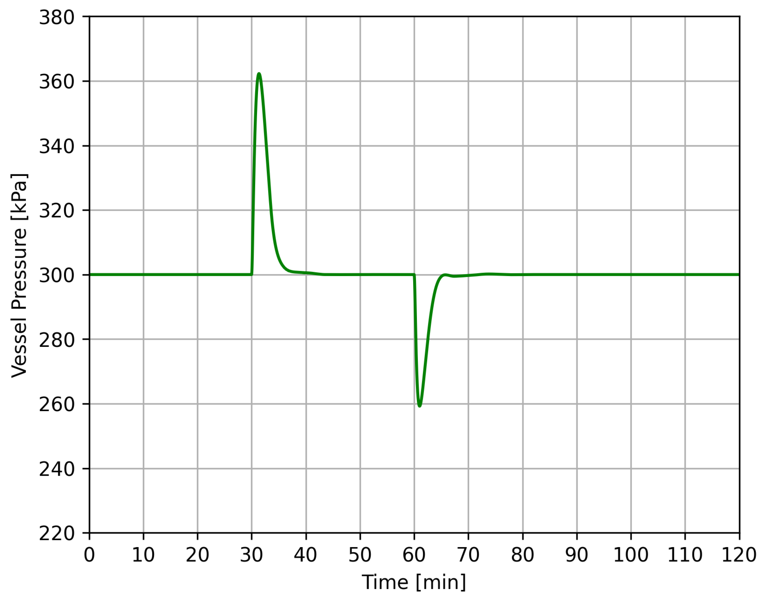
3.6.1. Vessel Pressure
3.6.2. Liquid Level
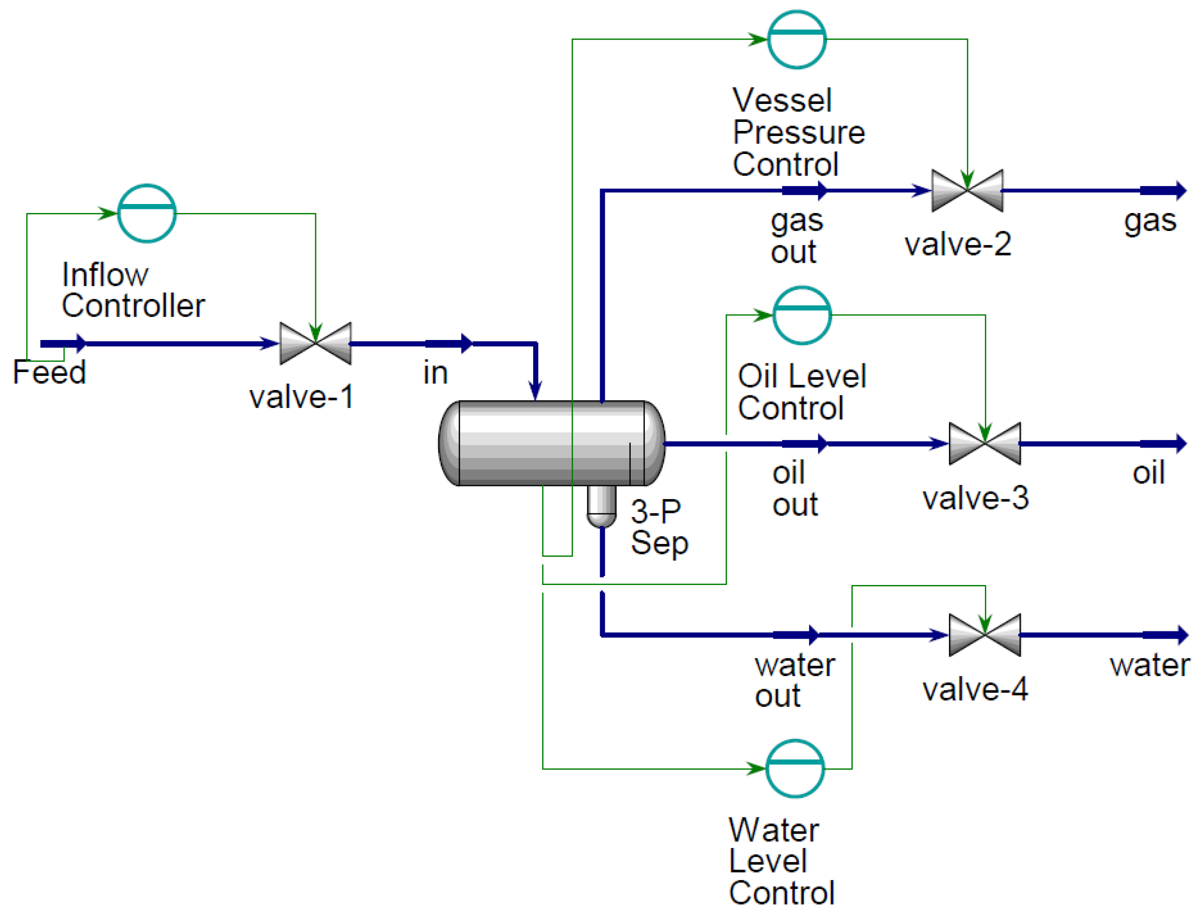
3.7. Process Controls
3.8. Gravity Settling
3.9. Critical Droplet Diameter for Separation
3.10. Initialization of Droplet Distribution
4. Simulation Results
4.1. Dynamic Simulation Scheme
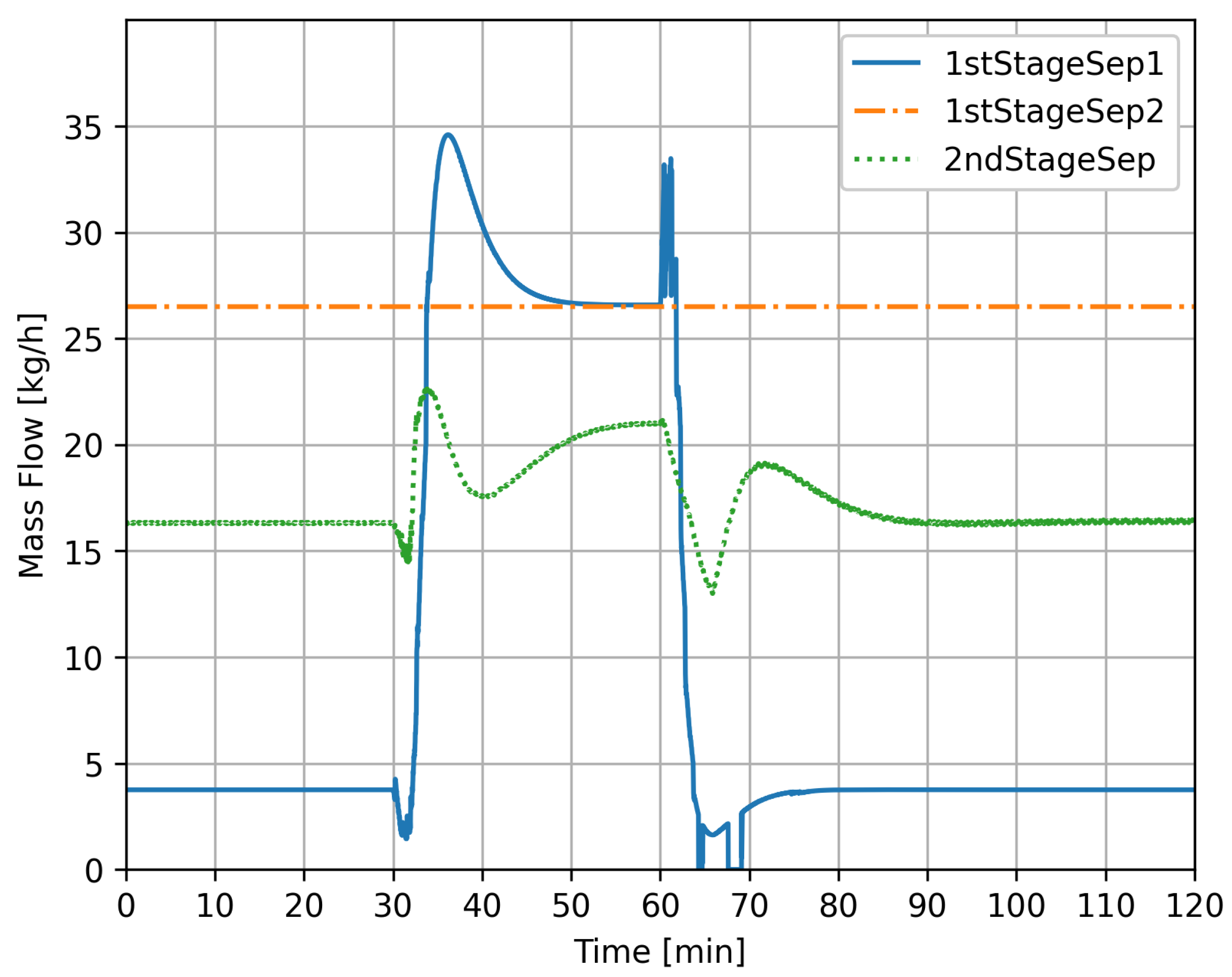
4.2. Case 1
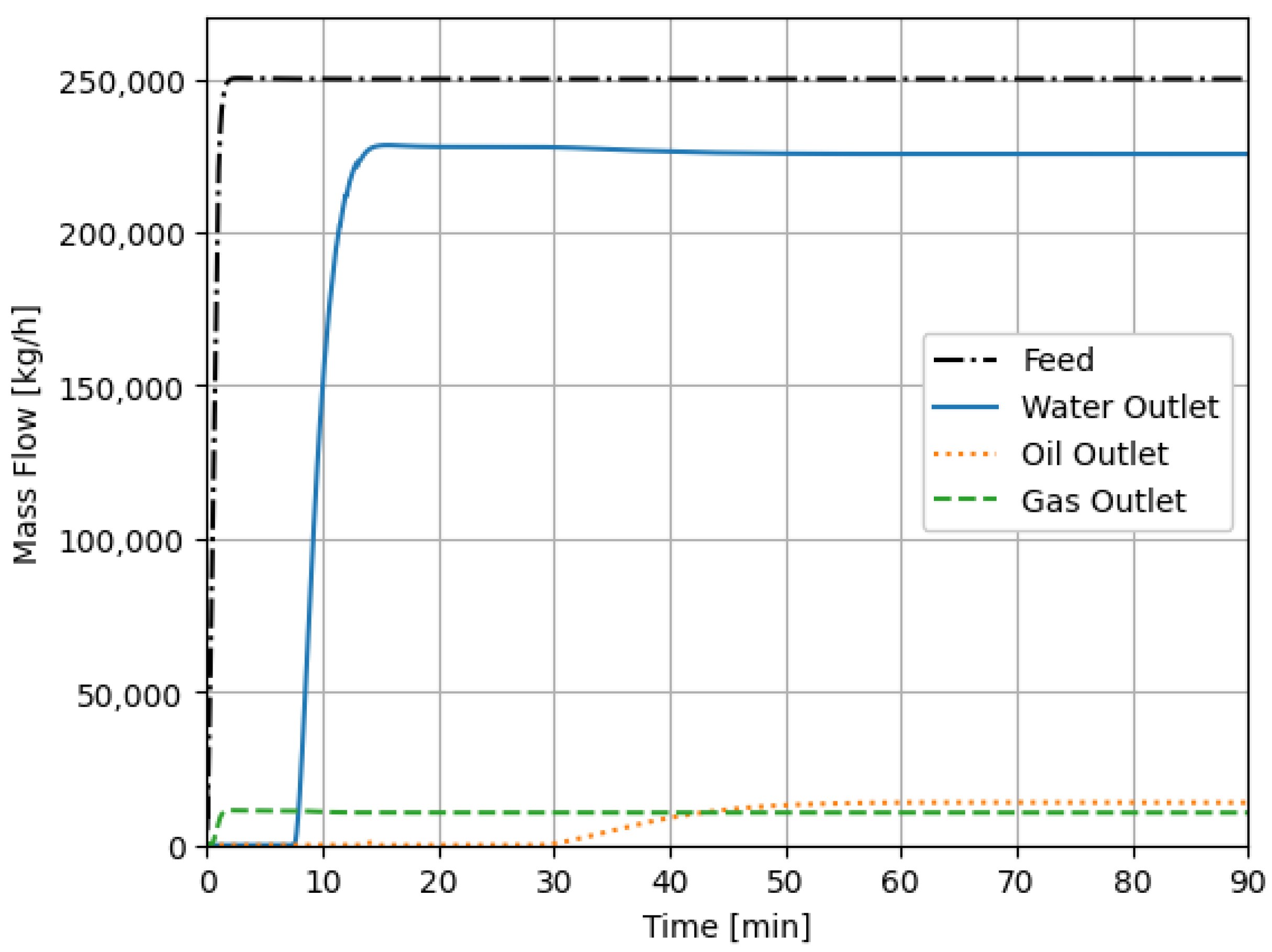
4.3. Case 2
5. Conclusions
Author Contributions
Funding
Conflicts of Interest
References
- Olsen, E.R.; Hooghoudt, J.-O.; Maschietti, M.; Andreasen, A. Optimization of an oil and gas separation plant for different reservoir fluids using an evolutionary algorithm. Energy Fuels 2021, 35, 5392–5406. [Google Scholar] [CrossRef]
- Mahmoud, M.; Tariq, Z.; Kamal, M.S.; Al-Naser, M. Intelligent prediction of optimum separation parameters in the multistage crude oil production facilities. J. Pet. Explor. Prod. Technol. 2019, 9, 2979–2995. [Google Scholar] [CrossRef]
- Schei, T.S.; Singstad, P.; Thunem, A.J. Transient Simulations of Gas-Oil-Water Separation Plants. Model. Identif. Control. 1991, 12, 27–46. [Google Scholar] [CrossRef]
- Brambilla, A.; Vaccari, M.; Pannocchia, G. Analytical RTO for a critical distillation process based on offline rigorous simulation. IFAC-PapersOnLine 2022, 55, 143–148. [Google Scholar] [CrossRef]
- Ahmed, T.; Makwashi, N.; Hameed, M. A review of gravity three-phase separators. J. Emerg. Trends Eng. Appl. Sci. 2017, 8, 143–153. [Google Scholar]
- Dionne, M.M. The Dynamic Simulation of a Three Phase Separator. Master’s Thesis, University of Calgary, Calgary, AB, Canada, 1998. [Google Scholar]
- Sayda, A.F.; Taylor, J.H. Modeling and control of three-phase gravilty separators in oil production facilities. In Proceedings of the IEEE 2007 American Control Conference, New York, NY, USA, 9–13 July 2007; pp. 4847–4853. [Google Scholar]
- Grimes, B.A. Population balance model for batch gravity separation of crude oil and water emulsions. part i: Model formulation. J. Dispers. Sci. Technol. 2012, 33, 578–590. [Google Scholar] [CrossRef]
- Backi, C.; Skogestad, S. A simple dynamic gravity separator model for separation efficiency evaluation incorporating level and pressure control. In Proceedings of the American Control Conference, Seattle, WA, USA, 24–26 May 2017; Volume 5. [Google Scholar]
- Song, S.; Liu, X.; Li, C.; Li, Z.; Zhang, S.; Wu, W.; Shi, B.; Kang, Q.; Wu, H.; Gong, J. Dynamic simulator for three-phase gravity separators in oil production facilities. ACS Omega 2023, 8, 6078–6089. [Google Scholar] [CrossRef] [PubMed]
- Abdulkadir, M.; Hernandez-Perez, V. The effect of mixture velocity and droplet diameter on oil-water separator using computational fluid dynamics (cfd). In Proceedings of the 7th International Conference on Heat Transfer, Fluid Mechanics and Thermodynamics, Antalya, Turkey, 19–21 July 2010; Volume 61, pp. 35–43. [Google Scholar]
- Hallanger, A.; Soenstaboe, F.; Knutsen, T. A Simulation Model for Three-Phase Gravity Separators. In Proceedings of the SPE Annual Technical Conference and Exhibition, Denver, CO, USA, 6–9 October 1996; Society of Petroleum Engineers: Richardson, TX, USA, 1996; Volume 10. [Google Scholar] [CrossRef]
- Laleh, A.P.; Svrcek, W.Y.; Monnery, W.D. Computational Fluid Dynamics-Based Study of an Oilfield Separator—Part II: An Optimum Design. Oil Gas Facil. 2013, 2, 52–59. [Google Scholar] [CrossRef]
- Ghaffarkhah, A.; Shahrabi, M.A.; Moraveji, M.K.; Eslami, H. Application of cfd for designing conventional three phase oilfield separator. Egypt. J. Pet. 2017, 26, 413–420. [Google Scholar] [CrossRef]
- Farajzadeh, R.; Zaal, C.; Van den Hoek, P.; Bruining, J. Life-cycle assessment of water injection into hydrocarbon reservoirs using exergy concept. J. Clean. Prod. 2019, 235, 812–821. [Google Scholar] [CrossRef]
- Azizov, I.; Dudek, M.; Øye, G. Emulsions in porous media from the perspective of produced water re-injection—A review. J. Pet. Sci. Eng. 2021, 206, 109057. [Google Scholar] [CrossRef]
- Aspen HYSYS: Process Simulation Software. Available online: https://www.aspentech.com/en/products/engineering/aspen-hysys (accessed on 7 February 2023).
- Andrade, G.M.; de Menezes, D.Q.; Soares, R.M.; Lemos, T.S.; Teixeira, A.F.; Ribeiro, L.D.; Vieira, B.F.; Pinto, J.C. Virtual flow metering of production flow rates of individual wells in oil and gas platforms through data reconciliation. J. Pet. Sci. Eng. 2022, 208, 109772. [Google Scholar] [CrossRef]
- Vaccari, M.; Pannocchia, G.; Tognotti, L.; Paci, M. Rigorous simulation of geothermal power plants to evaluate environmental performance of alternative configurations. Renew. Energy 2023, 207, 471–483. [Google Scholar] [CrossRef]
- Peng, D.-Y.; Robinson, D. New two-constant equation of state. Ind. Eng. Chem. Fundam. 1976, 15, 59–64. [Google Scholar] [CrossRef]
- Carrero, J. Beyond henry’s law in the gas—liquid equilibrium. ChemTexts 2021, 8, 1. [Google Scholar] [CrossRef]
- Arnold, K.; Stewart, M. Chapter 5—Three-phase oil and water separation. In Surface Production Operations, 3rd ed.; Arnold, K., Stewart, M., Eds.; Gulf Professional Publishing: Burlington, MA, USA, 2008; pp. 244–315. [Google Scholar]
- Kharoua, N.; Khezzar, L.; Saadawi, H. Cfd modelling of a horizontal three-phase separator: A population balance approach. Am. J. Fluid Dyn. 2013, 3, 101–118. [Google Scholar]
- Monnery, W.; Svrcek, W. Successfully specify three-phase separators. Chem. Eng. Prog. 1994, 90, 29–40. [Google Scholar]
- Liu, X.; Wang, Z.; Liu, L.; Wu, C.; Mao, Q. Experimental study on characteristics of oil particle distribution in water-gelled crude oil two-phase flow system. Adv. Mech. Eng. 2014, 6, 205860. [Google Scholar]


| Property | Value | Unit |
|---|---|---|
| Length | 12 | m |
| Diameter | 3 | m |
| Weir Height | 1.7 | m |
| Weir Position | 9.0 | m |
| Vapor Pressure Setpoint | 300 | kPa |
| Water Level Setpoint | 1.6 | m |
| Oil Outlet Setpoint * | 1 | m |
| Inlet Mass Flow Separator 1 | 150,000 | kg/h |
| Inlet Mass Flow Separator 2 | 250,000 | kg/h |
| Inlet Pressure Sep1 & Sep2 | 500 | kPa |
| Inlet Temp. Sep1 & Sep2 | 30 | °C |
| Property | Value | Unit |
|---|---|---|
| Height | 10 | m |
| Diameter | 10 | m |
| Vapor Pressure Setpoint | 220 | kPa |
| Water Level Setpoint | 2 | m |
| Oil Outlet Setpoint | 5 | m |
| Oil Nozzle Location (vertical) | 4.7 | m |
| Water Nozzle Location (vertical) | 0 | m |
| Property | Value | Unit |
|---|---|---|
| Height | 10 | m |
| Diameter | 15 | m |
| Vapor Pressure Setpoint | 160 | kPa |
| Water Level Setpoint | 3 | m |
| Oil Outlet Setpoint | 5.5 | m |
| Oil Nozzle Location (vertical) | 5 | m |
| Water Nozzle Location (vertical) | 0 | m |
| Compound | Mole Fraction |
|---|---|
| CH4 | 0.95 |
| N2 | 0.018 |
| CO2 | 0.0147 |
| H2S | 0.001 |
| C2H6 | 0.0128 |
| C3H8 | 0.0029 |
| i-C4H10 | 0.0001 |
| n-C4H10 | 0.0002 |
| i-C5H12 | 0.0002 |
| n-C5H12 | 0.0001 |
| Dynamic Scheme | Monitored Time Frame | Modified Value | Dynamic Event |
|---|---|---|---|
| Case 1 | 0–120 min | InletFlow 3P-Separator 1 (V-100) | 250,000 kg/h at 30 min–150,000 kg/h at 60 min Linear Ramp Duration: 2 min |
| Case 2 | 0–90 min | InletFlow 3P-Separator 2 (V-103) | 250,000 kg/h at 0 min Linear Ramp Duration: 2 min |
Disclaimer/Publisher’s Note: The statements, opinions and data contained in all publications are solely those of the individual author(s) and contributor(s) and not of MDPI and/or the editor(s). MDPI and/or the editor(s) disclaim responsibility for any injury to people or property resulting from any ideas, methods, instructions or products referred to in the content. |
© 2023 by the authors. Licensee MDPI, Basel, Switzerland. This article is an open access article distributed under the terms and conditions of the Creative Commons Attribution (CC BY) license (https://creativecommons.org/licenses/by/4.0/).
Share and Cite
Jonach, T.; Haddadi, B.; Jordan, C.; Harasek, M. Dynamic Simulation of a Gas and Oil Separation Plant with Focus on the Water Output Quality. Energies 2023, 16, 4111. https://doi.org/10.3390/en16104111
Jonach T, Haddadi B, Jordan C, Harasek M. Dynamic Simulation of a Gas and Oil Separation Plant with Focus on the Water Output Quality. Energies. 2023; 16(10):4111. https://doi.org/10.3390/en16104111
Chicago/Turabian StyleJonach, Thorsten, Bahram Haddadi, Christian Jordan, and Michael Harasek. 2023. "Dynamic Simulation of a Gas and Oil Separation Plant with Focus on the Water Output Quality" Energies 16, no. 10: 4111. https://doi.org/10.3390/en16104111
APA StyleJonach, T., Haddadi, B., Jordan, C., & Harasek, M. (2023). Dynamic Simulation of a Gas and Oil Separation Plant with Focus on the Water Output Quality. Energies, 16(10), 4111. https://doi.org/10.3390/en16104111