Development and Validation of the IAG Dynamic Stall Model in State-Space Representation for Wind Turbine Airfoils

Abstract

Considering the dynamic stall effects in engineering calculations is essential for correcting the aerodynamic loads acting on wind turbines, both during power production and stand-still cases, and impacts significantly the turbine aeroelastic stability. The employed dynamic stall model needs to be accurate and robust for a wide range of airfoils and range of angle of attack. The present studies are intended to demonstrate the performance of a recently implemented “IAG dynamic stall” model in a wind turbine design tool Bladed. The model is transformed from the indicial type of formulation into a state-space representation. The new model is validated against measurement data and other dynamic stall models in Bladed for various flow conditions and airfoils. It is demonstrated that the new model is able to reproduce the measured dynamic polar accurately without airfoil specific parameter calibration and has a superior performance compared to the incompressible Beddoes–Leishman model and the Øye model in Bladed.

1. Introduction

Dynamic stall can occur when there is a strong variation in the inflow conditions due to environmental effects and turbine operation strategy, e.g., yaw misalignment, wind turbulence, shear and gusts, tower shadow and strong aeroelastic effects of the blade. Studies clearly highlighted [1,2,3,4,5,6,7,8,9,10,11] that the aerodynamic loads can be significantly different than the stationary conditions. The dynamic stall phenomenon is usually initiated by an increase in lift with increasing angle of attack ($\alpha$) past the corresponding static stall angle. This is associated with the generation of a leading edge vortex (LEV). This vortical structure creates a suction effect which enhances the circulation effect on the airfoil [10]. LEV is further convected downstream toward the trailing edge. This causes a further increase in the lift and drag forces; at the same time, the pitching moment becomes more negative before stall occurs. The dynamic loads associated with the dynamic stall effects can significantly alter wind turbine loads and have a strong influence on the aerodynamic damping. As a direct consequence, considering the dynamic stall effects in engineering calculations is essential for correcting the aerodynamic loads acting on wind turbines, both during power production and stand-still cases. A correct representation of the aerodynamic force hysteresis is especially critical to accurately model the aerodynamic damping that has a significant impact on the turbine aeroelastic stability [12]. This is especially important for modern large rotors because the blade is longer, more flexible and more slender compared to older turbine designs.

Engineering modeling relies on dynamic stall models to include this complex phenomenon. These models can produce reasonable results while still maintaining low computational burden. The models from Beddoes and Leishman (BL) and their derivatives [13,14,15,16,17,18,19,20,21,22] are considered to be the industry standard for wind turbine design processes. The models are commonly derived by combining a time delay of the angle of attack with an approximate solution of flow separation during the dynamic conditions. The original BL model was dedicated to high speed aerodynamics applications and included the Mach number effects in most flow states. This model was further simplified by Hansen et al. [14] by removing the compressibility effects and transforming the model into a state-space representation. However, this model ignores the effect of the leading edge vortex by arguing that the airfoil thickness for wind turbines is no less than 15%. Examples of the other available models are provided by Øye [23], Tran and Petot (ONERA model) [24], Tarzanin (Boeing–Vertol model) [25] and Snel model [26]. Furthermore, the interest in modeling a higher harmonic effect of the dynamic stall polar is increasing nowadays. Snel model [26] is one of the few models that can be implemented to include the effect. This model was further extended in [27]. Bangga et al. [15] combined the state-of-the-art BL model and the second order term of the Snel model to predict the unsteady characteristics of wind turbine airfoils, hereby referred to as the “IAG dynamic stall model”. Several improvements were made to enhance the accuracy of the first order and the second order terms [15]. The first order term of the IAG model was built based on the indicial formulations while the second order term was derived using a state-space representation.

The wind turbine design tool Bladed [28] traditionally employs the incompressible version of the BL model with some modifications [14,28]. Although the adopted model works at moderate angles of attack, the performance of this type of model starts to deteriorate when it is used to predict deep stall conditions, which may lead to an incorrect prediction of the aerodynamic damping. The first order term of the IAG model was recently implemented in a development version of Bladed and this paper is intended to report the implementation and verification processes. The IAG model is transformed from the indicial type of formulation into a state-space representation, allowing the model to be linearized to enable steady-state stability analysis. In this paper, a consistent step-by-step procedure will be presented and the physical justification for the modifications applied will be highlighted. The new model is compared with other dynamic stall models in Bladed, including the widely used incompressible BL model [14,28] and Øye [23] and validated against measurement data of wind turbine airfoils with different relative thicknesses and flow conditions, allowing a full assessment of its suitability for different purposes. The main novelties of the present paper are:

• Transformation of the IAG dynamic stall model from the indicial formulation to the state-space representation.
• Improvements of the model robustness compared to the original IAG model. The present model is also constructed such that it contains fewer constants.
• Removal of the compressibility terms of the IAG dynamic stall model
• Extensive verification of the model for various data sets at different flow scenarios.
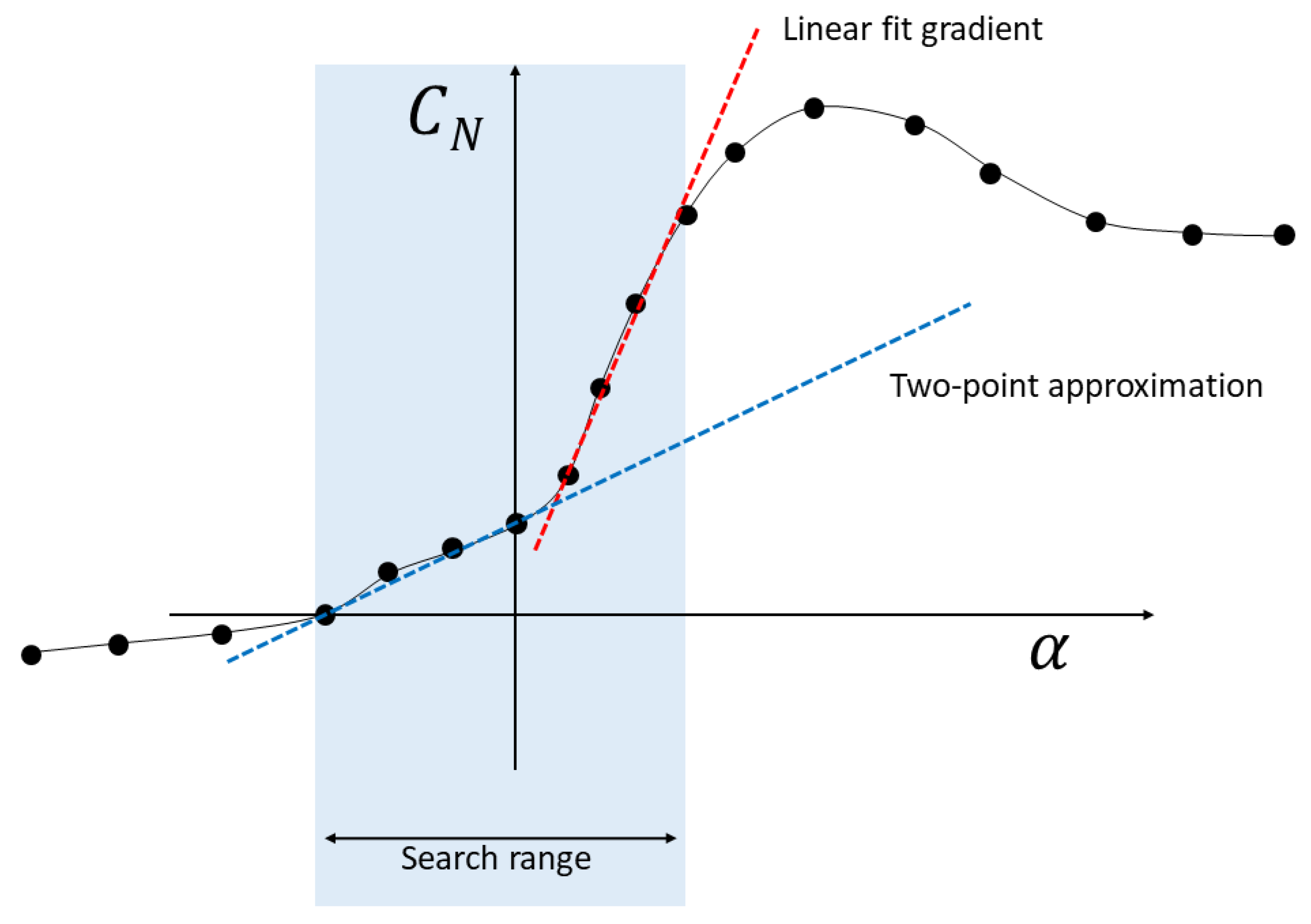
• Introduction of a method to automatically determinate the normal force gradient of a polar that is insensitive to data point outlier.
• Implementation of the IAG dynamic stall model in the wind turbine design tool Bladed.
• The present paper serves as the source of reference for academic readers interested in unsteady aerodynamics but also for engineering practitioners employing Bladed in designing and assessing their wind turbines.

The paper is organized as follows. Section 2 describes the mathematical formulation of the IAG model in the original indicial and the transformed state-space representations. An automated procedure to determine the polar gradient is also documented. Then, in Section 3 assessments are carried out on the performance of the IAG dynamic stall model in comparison with measurement data and other models. The new model is further tested at various flow conditions and airfoils without further calibrating the constants to examine its robustness for different situations. Finally, all results will be concluded in Section 4.

2. Mathematical Foundation

The IAG model [15] is comprised of a first order and second order model. The first order term is based the Beddoes–Leishman model [29,30] with some improvements. The second order term adopts the improved second order Snel model to accommodate the higher harmonic effects to be modeled. In this paper, the first order term will be the focus of the investigation because this determines the overall shape of the hysteresis curve. The modeling strategy of the first order term is divided into several aerodynamic states: (1) attached flow state, (2) separated flow state and (3) vortex lift state. The mathematical foundations to both implementation types are further described in Section 2.1 and Section 2.2. Here, the equations for the indicial version of the IAG model are rewritten in this paper to ensure a smooth discussion between two modeling types, allowing the description of the terms in a more consistent manner.

2.1. IAG Model in Indicial Formulation

The loads of the attached flow state are assumed to originate from two main sources: (a) the circulatory loading which quickly builds up to the steady state value and (b) impulsive loading which is derived from the piston theory. For a lifting surface exposed to unsteady change in the angle of attack ${\alpha }_n$, there is a time delay between the actual effective angle of attack (${\alpha }_{e_n}$) seen by the structure. This aspect can be represented as:

$$\begin{array}{c}\hfill {\alpha }_{e_n}={\alpha }_n-X_n-Y_n\end{array}$$

(1)

with n being the current sample time (current value of the actual angle of attack). The deficiency functions are described by:

$$\begin{array}{c}{X}_n=X_{n-1}\exp \left(-b_1{\beta }^2\Delta s\right)+A_1\Delta {\alpha }_n\exp \left(-b_1{\beta }^2\Delta s/2\right)\end{array}$$

(2)

$$\begin{array}{c}{Y}_n=Y_{n-1}\exp \left(-b_2{\beta }^2\Delta s\right)+A_2\Delta {\alpha }_n\exp \left(-b_2{\beta }^2\Delta s/2\right)\end{array}$$

(3)

Note that variable time is represented by a dimensionless parameter $s=2Vt/c$. This defines the relative distance traveled by the airfoil in terms of semi chord. The variables V, t and c describe the free stream wind speed, time and chord length, respectively. In this sense, $\Delta {\alpha }_n$ and $\Delta s$ are given by:

$$\begin{array}{c}\Delta {\alpha }_n={\alpha }_{n+1}-{\alpha }_n\end{array}$$

(4)

$$\begin{array}{c}\Delta s=s_n-s_{n-1}\end{array}$$

(5)

$$\begin{array}{c}\Delta t=t_n-t_{n-1}.\end{array}$$

(6)

Furthermore, $b_1$, $b_2$, $A_1$ and $A_2$ are defined as the attached flow constants. The compressibility effects are included in the formulation by adopting $\beta =\sqrt{1-M^2}$, with M being the Mach number.

The attached flow normal force coefficient is obtained by:

$$C_{N_n}^P=C_{N_n}^C+C_{N_n}^I,$$

(7)

which combines the circulatory and attached flow components. The circulatory normal force can be obtained using

$$C_{N_n}^C={\displaystyle \frac{d{C}_N}{d\alpha }}({\alpha }_{e_n}-{\alpha }_0^{INV})$$

(8)

with ${\alpha }_{0_{INV}}$ being the angle of attack for zero inviscid normal force and $d{C}_N/d\alpha$ being the normal force gradient of the polar data within the linear regime. This is in contrast with the original implementation of the Beddoes–Leishman model [29,30] which disregarded the use of ${\alpha }_0^{INV}$. However, this term is important when the airfoil has a finite camber. This has been pointed out as well by Hansen et al. [14]. The impulsive normal force is calculated based on

$$C_{N_n}^I={\displaystyle \frac{4K_{\alpha }{T}_I}{M}}\left({\displaystyle \frac{\Delta {\alpha }_n}{\Delta t}}-D_n\right).$$

(9)

with $T_I=Mc/V$. $D_n$ represents the deficiency function and is given by

$$D_n=D_{n-1}\exp \left({\displaystyle \frac{-\Delta t}{K_{\alpha }{T}_I}}\right)+\left({\displaystyle \frac{\Delta {\alpha }_n-\Delta {\alpha }_{n-1}}{\Delta t}}\right)\exp \left({\displaystyle \frac{-\Delta t}{2K_{\alpha }{T}_I}}\right),$$

(10)

with $K_{\alpha }$ being a constant for determining the strength of the impulsive normal force effect.

To obtain the value of the unsteady viscous normal force, the Kirchhoff equation is used to reconstruct the aerodynamic properties as:

$$C_{N_n}^f={\displaystyle \frac{d{C}_N}{d\alpha }}{\left({\displaystyle \frac{1+\sqrt{f_{2_n}}}{2}}\right)}^2({\alpha }_{e_n}-{\alpha }_0^{VISC})+C_{N_n}^I.$$

(11)

Note that the impulsive normal force effect is included in the formulation. Also notice that the zero normal force angle of attack for viscous polar data (${\alpha }_{0_{VISC}}$) is used here. In the original formulation of the IAG model [15], the attached flow data are obtained from the inviscid panel-method XFOIL calculations; thus, the zero normal force angle of attack can be different with the value obtained from the viscous polar data.

The unsteady trailing edge separation point ($f_{2_n}$) in Equation (11) is obtained from:

$$f_{2_n}=f_n-D_{f_n},$$

(12)

which depends on two parameters $f_n$ and $D_{f_n}$. The first parameter is defined by an inverse Kirchhoff equation as:

$$f_n={\left(2\sqrt{{\displaystyle \frac{C_{N_n}^{VISC}}{{\displaystyle \frac{d{C}_N}{d\alpha }}({\alpha }_{f_n}-{\alpha }_0^{VISC})}}}-1.0\right)}^2,$$

(13)

and can be computed based on the pressure lag response of the angle of attack:

$${\alpha }_{f_n}={\alpha }_0^{INV}+\left({\displaystyle \frac{C_{N_n}^{P1}}{d{C}_N/d\alpha }}\right).$$

(14)

with

$$C_{N_n}^{P1}=C_{N_n}^P-D_{p_n},$$

(15)

and $D_{p_n}$ being represented as:

$$D_{p_n}=D_{p_{n-1}}\exp \left(-{\displaystyle \frac{\Delta s}{T_p}}\right)+\left(C_{N_n}^P-C_{N_{n-1}}^P\right)\exp \left(-{\displaystyle \frac{\Delta s}{2T_p}}\right).$$

(16)

The last term of Equation (12) is given by the following time-dependent equation (which also depends on $f_n$):

$$D_{f_n}=D_{f_{n-1}}\exp \left(-{\displaystyle \frac{\Delta s}{T_f}}\right)+\left(f_n-f_{n-1}\right)\exp \left(-{\displaystyle \frac{\Delta s}{2T_f}}\right).$$

(17)

The parameters $T_p$ and $T_f$ are the constants for determining the pressure lag and flow separation effects, respectively.

The last part of the first order term represents the vortex lift effect which can be computed by:

$$C_{N_n}^V=\left\{\begin{array}{c}{C}_{N_{n-1}}^V\exp \left(-{\displaystyle \frac{\Delta s}{T_v}}\right)+\left(C_{V_n}-C_{V_{n-1}}\right)\exp \left(-{\displaystyle \frac{\Delta s}{2T_v}}\right);\hfill \\ \hfill & \mathrm{if}0<{\tau }_{v_n}<T_{vl}\hfill \\ C_{N_{n-1}}^V\exp \left(-{\displaystyle \frac{\Delta s}{T_v}}\right);\hfill & \mathrm{otherwise}\hfill \end{array}\right.$$

(18)

Notice that Equation (18) depends on the value of $C_{V_n}$ and this can be estimated from the circulatory normal force effect as:

$$C_{V_n}=C_{N_n}^C\left(1-{\displaystyle \frac{1}{4}}{\left(1+\sqrt{f_{2_n}}\right)}^2\right)$$

(19)

Variables $T_v$ and $T_{vl}$ represent the vortex decay and vortex travel time constants, respectively. The non-dimensional vortex time (${\tau }_{v_n}$) itself is important for determining the vortex lift influence and can be calculated using

$${\tau }_{v_n}=\left\{\begin{array}{cc}{\tau }_{v_{n-1}}+0.45{\displaystyle \frac{\Delta t}{c}}V;\hfill & \mathrm{if}{C}_{N_n}^{P1}>C_N^{CRIT}\hfill \\ 0;\hfill & \mathrm{if}{C}_{N_n}^{P1}<C_N^{CRIT}\mathrm{and}\Delta {\alpha }_n\ge 0\hfill \\ {\tau }_{v_{n-1}};\hfill & \mathrm{otherwise}\hfill \end{array}\right.$$

(20)

$C_N^{CRIT}$ is an important parameter which defines the inviscid critical static normal force. This is usually indicated by the break of the pitching moment polar at the critical angle of attack ${\alpha }_n^{CRIT}$. The magnitude of $C_N^{CRIT}$ can be computed as:

$$C_N^{CRIT}={\displaystyle \frac{d{C}_N}{d\alpha }}({\alpha }_n^{CRIT}-{\alpha }_0^{INV}).$$

(21)

The total normal force contribution can be obtained by computing

$$C_{N_n}^D=C_{N_n}^f+C_{N_n}^V.$$

(22)

In the IAG model, the tangential (chordwise) force is simply obtained from the static polar data at the time-lagged angle of attack ${\alpha }_{f_n}$ by:

$$C_{T_n}^D=C_T^{VISC}\left({\alpha }_{f_n}\right).$$

(23)

Finally, the lift and drag forces can be computed as:

$$\begin{array}{c}{C}_{L_n}^D=C_{N_n}^D\cos {\alpha }_n-C_{T_n}^D\sin {\alpha }_n\end{array}$$

(24)

$$\begin{array}{c}{C}_{D_n}^D=C_{N_n}^D\sin {\alpha }_n+C_{T_n}^D\cos {\alpha }_n\end{array}$$

(25)

In the IAG model, a limiter is applied to the drag force to correct the hysteresis effects. This is done through a parameter ${\zeta }_n$ which is defined as:

$${\zeta }_n=\frac{1}{\pi }{\displaystyle \frac{d{C}_N}{d\alpha }}{\left({\displaystyle \frac{1+\sqrt{f_n}}{2}}\right)}^2.$$

(26)

Drag hysteresis is observed to occur when ${\zeta }_n\lesssim {\zeta }_v$, with ${\zeta }_v$ being a constant with a value of 0.76. The adopted correction reads:

$$C_{D_n}^D=\left\{\begin{array}{cc}1.2C_{D_n}^{VISC};\hfill & \mathrm{if}{C}_{D_n}^D>1.2C_{D_n}^{VISC} \mathrm{and}\left(C_{N_n}^P-C_{N_{n-1}}^P\right)\ge 0.0\hfill \\ \\ C_{D_n}^{VISC};\hfill & \mathrm{if}\left(C_{N_n}^P-C_{N_{n-1}}^P\right)<0.0\hfill \\ \\ C_{D_n}^D;\hfill & \mathrm{otherwise}\hfill \end{array}\right.$$

(27)

As for the pitching moment coefficient, the total dynamic response obtained from all contributions is obtained by computing

$$C_{M_n}^D=C_{M_n}^f+C_{M_n}^V+C_{M_n}^C$$

(28)

where the separated, vortex and circulatory contributions of the pitching moments are defined by $C_{M_n}^f$, $C_{M_n}^V$ and $C_{M_n}^C$, respectively.

In the original Beddoes–Leishman formulation, the pitching moment was obtained by a curve fitting procedure. This is not straightforward as the user needs to perform curve fitting of the polar data. In the IAG model, the separated moment coefficient is easily obtained from the static viscous polar data at ${\alpha }_{f_n}$ that reads

$$C_{M_n}^f=C_M^{VISC}\left({\alpha }_{f_n}\right).$$

(29)

In this sense, the moment coefficient can be reconstructed easily without the need to adjust the parameters in advance, minimizing the user error. The vortex contribution of the dynamic moment coefficient can be formulated as

$$C_{M_n}^V=-C_{P{v}_n}{C}_{N_n}^V.$$

(30)

This depends on the idealized variation of the center of pressure and can be estimated as

$$C_{P{v}_n}=K_v\left(1-\cos \left({\displaystyle \frac{\pi {\tau }_v}{T_{vl}}}\right)\right).$$

(31)

The last term represents the circulatory moment. To model this, a relatively simple approach is introduced by applying a time delay on the circulatory moment response as:

$$C_{M_n}^C=\left\{\begin{array}{c}{C}_{M_{n-1}}^C\exp \left(-{\displaystyle \frac{\Delta s}{T_M^U}}\right)-C_{P{f}_n}\left(C_{V_n}-C_{V_{n-1}}\right)\exp \left(-{\displaystyle \frac{\Delta s}{2T_M^U}}\right);\hfill \\ \mathrm{if}{\tau }_{v_n}<T_{vl}\mathrm{and}\Delta {\alpha }_n\ge 0\hfill \\ C_{M_{n-1}}^C\exp \left(-{\displaystyle \frac{\Delta s}{T_M^D}}\right)-C_{P{f}_n}\left(C_{V_n}-C_{V_{n-1}}\right)\exp \left(-{\displaystyle \frac{\Delta s}{2T_M^D}}\right);\hfill \\ \mathrm{if}\Delta {\alpha }_n<0\hfill \\ C_{M_{n-1}}^C;\mathrm{otherwise}\hfill \end{array}\right.$$

(32)

where,

$$C_{P{f}_n}=K_f^C{\displaystyle \frac{d{C}_N}{d\alpha }}({\alpha }_n^{CRIT}-{\alpha }_0^{INV}).$$

(33)

with $K_f^C$, $T_M^U$ and $T_M^D$ being constants relatively insensitive to airfoils.

2.2. IAG Model in State-Space Representation

In the present paper, the IAG model is transformed into a state-space formulation. The main modeling strategy is similar to the incompressible Beddoes–Leishman model [14]. However, the formulations are defined in forms of the normal force coefficient, in contrast to Ref. [14] which used the lift coefficient directly. The same principles are adopted as in the indicial formulations, i.e., dividing the solutions into attached flow, separated flow and vortex lift states.

The attached flow solutions are represented into two ordinary differential equations (ODEs) which are comparable to the deficiency functions already presented in Section 2.1. These are described by:

$$\begin{array}{c}\left(\frac{c}{2V}\right){\dot{x}}_1\left(t\right)=b_1{A}_1{\alpha }_n^{3/4}-\left[b1+\left(\frac{c\dot{V}}{V^2}\right)\right]x_1\left(t\right)\end{array}$$

(34)

$$\begin{array}{c}\left(\frac{c}{2V}\right){\dot{x}}_2\left(t\right)=b_2{A}_2{\alpha }_n^{3/4}-\left[b2+\left(\frac{c\dot{V}}{V^2}\right)\right]x_2\left(t\right)\end{array}$$

(35)

Here, $x_{1,2}\left(t\right)$ and ${\dot{x}}_{1,2}\left(t\right)$ represent the state and the state derivative of the ODEs, respectively. Note that the definition of the angle of attack being adopted in the ODEs uses the angle of attack measured at the collocation point (3/4 of the chord measured from the leading edge). This has no influence for two-dimensional pitching airfoil but can be different with the quarter chord position for wind turbine blade sections affected by structural flexibility. As suggested in [14], the added mass term $\left(\frac{c\dot{V}}{V^2}\right)$ is added to include the effects for varying wind speed in wind turbine cases. The effective angle of attack is calculated using:

$$\begin{array}{c}\hfill {\alpha }_{e_n}={\alpha }_n^{3/4}(1-A_1-A_2)+x_1\left(t\right)+x_2\left(t\right)\end{array}$$

(36)

The circulatory normal force can be obtained using

$$C_{N_n}^C={\displaystyle \frac{d{C}_N}{d\alpha }}sin({\alpha }_{e_n}-{\alpha }_0^{VISC}).$$

(37)

Note that Equation (37) looks different compared to Equation (8). One difference is that it uses ${\alpha }_0^{VISC}$ instead of ${\alpha }_0^{INV}$. Although the magnitude of these two parameters can be different depending on the airfoils, the usage of the inviscid value is not convenient because users need to provide two polar data inputs, one the static viscous data and the other the inviscid data (e.g., from XFOIL). The second key difference is the usage of a sinusoidal form to determine the force. This is beneficial for high angle of attack calculations since data demonstrate that a linear model does not capture the nonlinear inviscid effects. An illustration of the effects for lift is given in Figure 1.

To add the contribution for the impulsive effect, Equation (9) can be used. Two options can be adopted in this sense, either by transforming the deficiency function in Equation (10) as a state-space representation or completely disregarding the Mach number. The latter is chosen because this implies that $D_n$ will be zero. As a consequence, it reduces the number of states to be solved by the integrator, i.e., faster computational speed. This is formulated as:

$$C_{N_n}^I=\frac{4K_{\alpha }c}{V}{\dot{\alpha }}_n.$$

(38)

Finally, the attached flow normal force coefficient is obtained by:

$$C_{N_n}^P=C_{N_n}^C+C_{N_n}^I.$$

(39)

The next set of ODE is used to determine the time-lagged pressure response of the normal force, as similarly done in Equation (15). This is formulated as:

$$\begin{array}{c}\left(\frac{c}{2V}\right)T_p{\dot{x}}_3\left(t\right)=-x_3\left(t\right)+C_{N_n}^P.\end{array}$$

(40)

Variable $x_3\left(t\right)$ is the solution for the pressure-lagged normal force or $C_{N_n}^{P1}$ in Equation (15). This parameter is used to calculate the delayed angle of attack

$${\alpha }_{f_n}={\alpha }_0^{VISC}+\left({\displaystyle \frac{x_3\left(t\right)}{d{C}_N/d\alpha }}\right).$$

(41)

By using the inverse of the Kirchoff equation, the position of separation point at ${\alpha }_{f_n}$ can be determined by:

$$f_n={\left(2\sqrt{{\displaystyle \frac{C_{N_n}^{VISC}}{{\displaystyle \frac{d{C}_N}{d\alpha }}sin({\alpha }_{f_n}-{\alpha }_0^{VISC})}}}-1.0\right)}^2.$$

(42)

Again, a sinusoidal approximation is also adopted in Equation (42). This leads to the fourth state-space equation to further delay the obtained separation position as:

$$\begin{array}{c}\left(\frac{c}{2V}\right)T_f{\dot{x}}_4\left(t\right)=-x_4\left(t\right)+f_n,\end{array}$$

(43)

which is comparable to Equation (12).

The unsteady viscous normal force can be reconstructed using the Kirchhoff equation as already done in Equation (11). However, here a sinusoidal approximation is consistently adopted instead of using a linear model and is denoted as:

$$C_{N_n}^f={\displaystyle \frac{d{C}_N}{d\alpha }}{\left({\displaystyle \frac{1+\sqrt{x_4\left(t\right)}}{2}}\right)}^{2}sin({\alpha }_{e_n}-{\alpha }_0^{VISC})+C_{N_n}^I.$$

(44)

Note that $x_4\left(t\right)$ in Equation (44) is comparable to $f_{2_n}$ in Equation (11).

The last term to consider is the vortex lift effect due to the presence of the leading edge vortex. Similar to the description in Section 2.1, this is calculated by the following ODE:

$$\begin{array}{c}\left(\frac{c}{2V}\right)T_v{\dot{x}}_5\left(t\right)=-x_5\left(t\right)+\left(\frac{c}{2V}\right)T_v{\dot{C}}_{V_n},\end{array}$$

(45)

with $x_5\left(t\right)$ specifying the normal force due to the vortex lift effect, which equals $C_{N_n}^V$ in Equation (18). To solve this equation, information about the rate of change of $C_{V_n}$ is needed. To do so, by applying a chain rule, a time derivative of Equation (19) is calculated as:

$${\dot{C}}_{V_n}={\displaystyle \frac{d{C}_N}{d\alpha }}{\dot{\alpha }}_{e_n}\left(1-{\displaystyle \frac{1}{4}}{\left(1+\sqrt{x_4\left(t\right)}\right)}^2\right)-{\displaystyle \frac{1}{4}}{C}_{N_n}^C\left(1+\sqrt{x_4\left(t\right)}\right)\frac{{\dot{x}}_4\left(t\right)}{\sqrt{x_4\left(t\right)}}.$$

(46)

Equation (46) is only applied when there is a dynamic vortex state active; otherwise, ${\dot{C}}_{V_n}=0$. The vortex state itself is defined when $x_3\left(t\right)$ is greater/smaller than the critical normal force:

$$C_N^{CRIT}=\left\{\begin{array}{cc}{C}_N^{MAX};\hfill & \mathrm{if}\mathrm{Positive}\mathrm{Stall}\hfill \\ C_N^{MIN};\hfill & \mathrm{if}\mathrm{Negative}\mathrm{Stall}\hfill \end{array}\right.$$

(47)

which refers to the maximum normal force (or minimum depending on the case) obtained from the static data. This is different with Equation (21) and the effect will be discussed in Section 3.2. Another important consideration to activate ${\dot{C}}_{V_n}$ is that it has to be during the upstroke motion. This implies that:

$$\mathrm{Vortex}\mathrm{state}=\left\{\begin{array}{cc}\mathrm{True};\hfill & \mathrm{if}\mathrm{Upstroke}\&x_3\left(t\right)>C_N^{CRIT}\&0<{\tau }_{v_n}<T_{vl}\hfill \\ \mathrm{False};\hfill & \mathrm{otherwise}\hfill \end{array}\right.$$

(48)

The upstroke state can be determined by $\Delta {\alpha }_n$, but this will be different when the case being considered is positive stall ($\Delta {\alpha }_n>0$) or negative stall ($\Delta {\alpha }_n<0$). A positive stall case can be identified when $x_3\left(t\right)\ge 0$, while a negative stall case may be detected when $x_3\left(t\right)<0$. For the backwinded case (when $\parallel \alpha \parallel$ is greater than 90${}^{\circ }$), the definition of upstroke is flipped. Now, the non-dimensional vortex time may be calculated using

$${\tau }_{v_n}=\left\{\begin{array}{cc}{\tau }_{v_{n-1}}+0.45{\displaystyle \frac{\Delta t}{c}}V;\hfill & \mathrm{if}\mathrm{Vortex}\mathrm{state}\hfill \\ {\tau }_{v_{n-1}}exp\left(-{\displaystyle \frac{\Delta t}{c}}V\right);\hfill & \mathrm{otherwise}\hfill \end{array}\right.$$

(49)

The second term is only adopted to avoid a sharp jump of the value numerically and may be set to zero in the implementation if desired. For very large angle of attack approaching 90${}^{\circ }$, it is assumed that the vortex lift effect vanishes. Therefore, the value is slowly relaxed toward zero from 45${}^{\circ }$ to 75${}^{\circ }$. This consideration is based on the fact that lift generally increases again after stall up to a full flow separation at around 60${}^{\circ }$, see, e.g., [31].

Similar to the indicial formulation in Section 2.1, the total normal force contribution can be obtained by computing

$$C_{N_n}^D=C_{N_n}^f+C_{N_n}^V.$$

(50)

On top of that, the tangential (chordwise) force is obtained directly from the static polar data at the time-lagged angle of attack ${\alpha }_{f_n}$ by:

$$C_{T_n}^D=C_T^{VISC}\left({\alpha }_{f_n}\right).$$

(51)

In the present model, only lift coefficient is calculated from $C_{N_n}^D$ and $C_{T_n}^D$ transformation as:

$$\begin{array}{c}{C}_{L_n}^D=C_{N_n}^D\cos {\alpha }_n-C_{T_n}^D\sin {\alpha }_n.\end{array}$$

(52)

The calculation for drag coefficient is done differently by applying the following relation:

$$\begin{array}{cc}{C}_{D_n}^D=\hfill & C_{D_n}^{VISC}+\left({\alpha }_n-{\alpha }_{e_n}\right)C_{N_n}^C\hfill \\ & +\left(C_{D_n}^{VISC}-C_{D_0}^{VISC}\right)\left[{\left(\frac{1-\sqrt{x_4\left(t\right)}}{2}\right)}^2-{\left(\frac{1-\sqrt{f^{VISC}}}{2}\right)}^2\right]+x_5\left(t\right)sin{\alpha }_n\hfill \end{array}$$

(53)

In Equation (53), variables $C_{D_n}^{VISC}$, $C_{D_0}^{VISC}$ and $f^{VISC}$ represent the static value of drag coefficient, drag level at zero normal force angle of attack and static separation position, respectively. Furthermore, it is assumed that drag force shows strong hysteresis only near stall regime. Therefore, the magnitude of drag is returned to the static value once the angle of attack is greater than 30${}^{\circ }$. This is done through a linear blending up to 45${}^{\circ }$. Note that a sudden drag increase occurs during stall and this takes place at $\parallel \alpha \parallel <{30}^{\circ }$ for most airfoils.

Lastly, the pitching moment coefficient is calculated in a manner similar to the indicial representation in Equation (54) that reads:

$$C_{M_n}^D=C_{M_n}^f+C_{M_n}^V+C_{M_n}^C.$$

(54)

However, the last term is not computed based on two deficiency function as in Equation (32) to avoid unnecessary computational effort. This is modeled as an added mass instead, which can be defined as:

$$C_{M_n}^C=-\frac{\pi c{\dot{\alpha }}_n}{4V}.$$

(55)

For backwinded airfoil orientation (when $\parallel \alpha \parallel$ is greater than 90${}^{\circ }$), the sign of Equation (55) becomes positive. The calculations for $C_{M_n}^f$ and $C_{M_n}^V$ are exactly the same as done in Equations (29) and (30), respectively. Similar to the drag coefficient, the magnitude of the pitching moment is returned to the static value once the angle of attack is greater than 30${}^{\circ }$ through a linear blending with the static data.

2.3. Adopted Constants

The following constants are applied in the tested IAG dynamic stall model. These values are kept constant throughout the paper and are listed in

Table 1. Constants applied for the IAG models.

Model	${\mathit{A}}_1$	${\mathit{A}}_2$	${\mathit{b}}_1$	${\mathit{b}}_2$	${\mathit{K}}_{\mathit{\alpha }}$	${\mathit{T}}_{\mathit{p}}$	${\mathit{T}}_{\mathit{f}}$	${\mathit{T}}_{\mathit{v}}$	${\mathit{T}}_{\mathbf{vl}}$	${\mathit{K}}_{\mathit{v}}$	${\mathit{K}}_{\mathit{f}}^{\mathit{C}}$	${\mathit{T}}_{\mathit{m}}^{\mathit{U}}$	${\mathit{T}}_{\mathit{m}}^{\mathit{D}}$	${\mathit{\zeta }}_{\mathit{v}}$
Indicial IAG	0.3	0.7	0.7	0.53	0.75	1.7	3.0	6.0	6.0	0.2	0.1	1.5	1.5	0.76
State-Space IAG	0.3	0.7	0.7	0.53	0.75	1.7	3.0	6.0	6.0	0.2	N/A	N/A	N/A	N/A

. Note that the state-space IAG model has fewer constants compared to the indicial one (no $K_f^C$, $T_m^U$, $T_m^D$ and ${\zeta }_s$). For the indicial IAG dynamic stall model, the critical angle of attack plays a major role and the values are given explicitly in

Table 2. Critical angle of attack (${\alpha }_n^{CRIT}$) applied for the IAG models.

Model	S801	S809	S814
Indicial IAG	15.1${}^{\circ }$	14.1${}^{\circ }$	10${}^{\circ }$
State-Space IAG	Automatic	Automatic	Automatic

. This corresponds to the angle when the viscous pitching moment breaks. In contrast, this information is not required in the newly implemented state-space IAG model because the values are determined automatically based on the maximum viscous normal force coefficient.

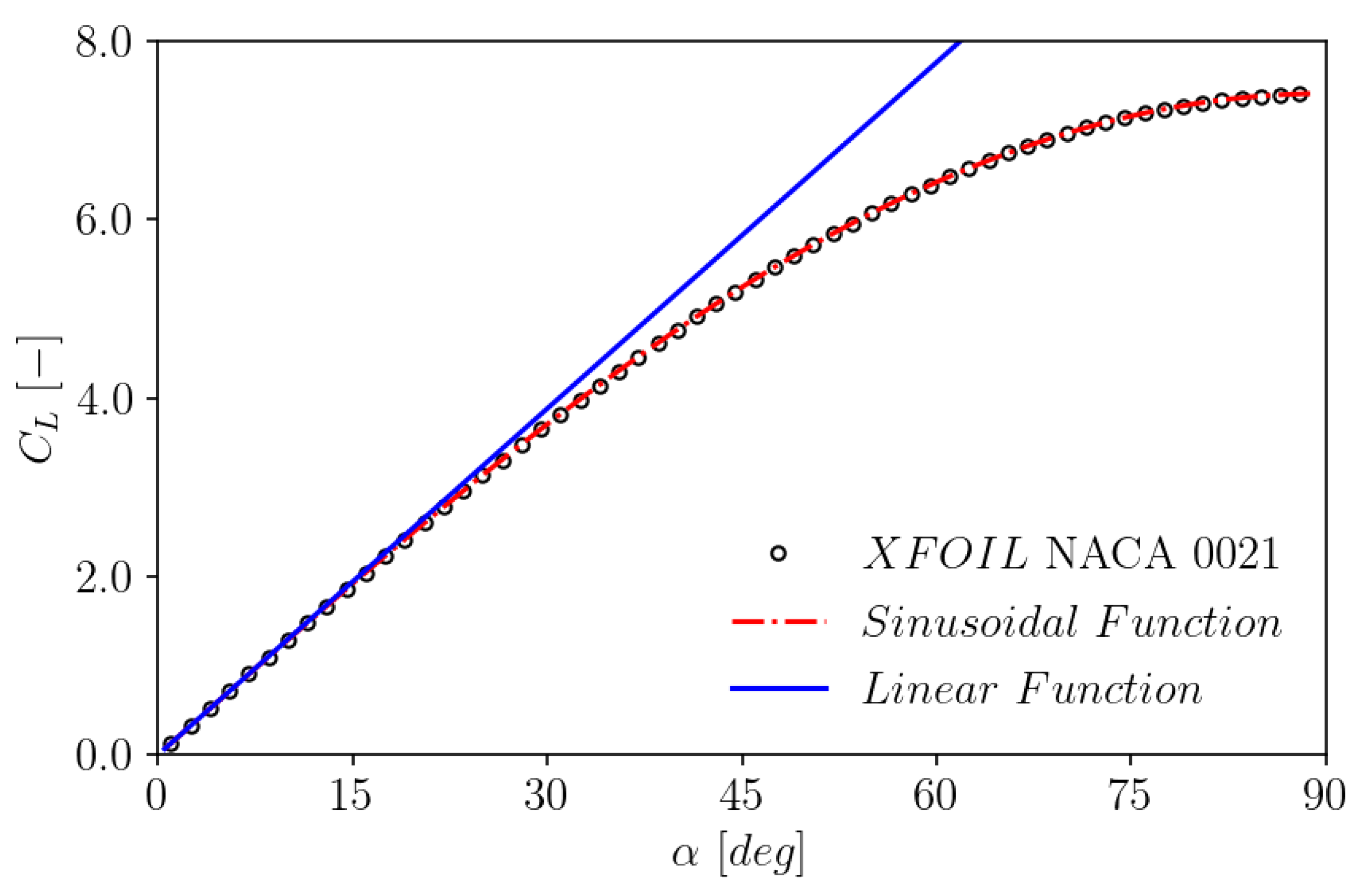
2.4. Automatic Determination of the Normal Force Gradient

Traditionally, Bladed determines the normal force gradient by using a two-point approximation. This approach takes the gradient computed between two distinct points of the polar data: (1) when $C_N=0$ and (2) when $\alpha =0$. This approach works for most airfoils but the validity breaks when there is a gradient change between these two distinct points as illustrated in Figure 2. To cover this aspect, a new method called the “linear fit approach” is adopted by incorporating more data points for determining the normal force gradient. First of all, local gradients for all data point between ${\alpha }_0^{VISC}$ and $\alpha =7^{\circ }$ are computed. Within this area, it is assumed that the flow is mostly attached. From the obtained gradients, all data points are binned and only the points with gradients between $1.8\pi$ and $2.5\pi$ are retained. A linear fit is then searched using the obtained points to find the most appropriate gradient of the polar data.

3. Results and Discussion

3.1. Test Cases and Treatment of the Input Data

The present studies were carried out based on the experimental data obtained from the measurement campaign conducted at Ohio State University (OSU) [5,6,7,8]. The calculations were conducted mainly on Selig airfoil family developed specially for wind turbine applications. Most discussions in this paper are focused on the S809 airfoil having 21% relative thickness ($\delta /c$), but are also extended for the S801 ($\delta /c=13.5\%$) and S814 ($\delta /c=24\%$) airfoils to evaluate the influence of the airfoil thickness. The evaluations of the results are performed on the airfoil with the Reynolds numbers ($Re$) 0.75 × 10${}^6$, 1.0 × 10${}^6$ and 1.25 × 10${}^6$ according to the available measurement data. Note that unless stated otherwise, the figures presented in subsequent sections correspond to the Reynolds number 0.75 × 10${}^6$ case. Most test cases are for the airfoils employed with a leading edge grit (turbulator) to enable the “soiled” effects on a wind turbine blade unless stated otherwise.

Generally, it is a common practice to replicate the experimental campaign of dynamic stall by applying a sinusoidal pitching motion in the simulation environment. However, this contains some uncertainty because it is not always possible to have a perfect sinusoidal motion in the experiment. This has been demonstrated by Bangga et al. [15] and they devised that this can lead to an additional discrepancy contribution. On the other hand, the oscillator orientation angle is not always recorded in fine resolution, making it not possible to supply the data directly into the simulation environment. A cubic fitting on the inflow data was found to best represent the inflow time series [15] and this is also highlighted in Figure 3. Therefore, the same procedure is adopted in the present paper to obtain the best consistent setup with the experimental campaign.

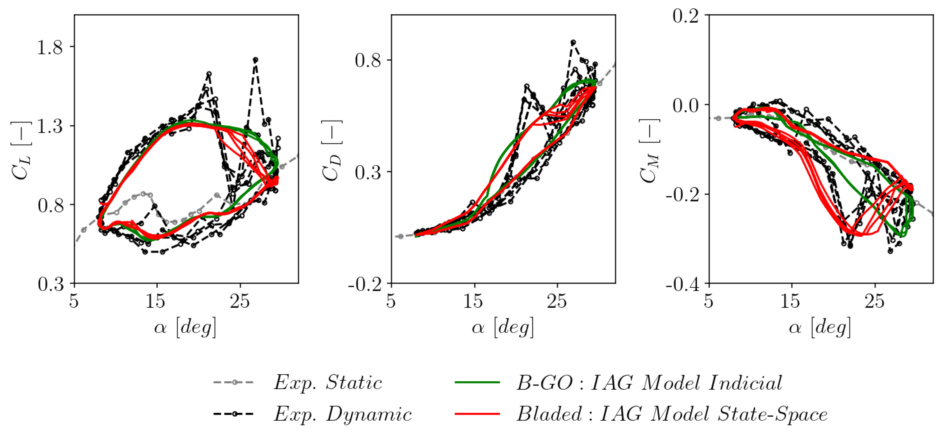
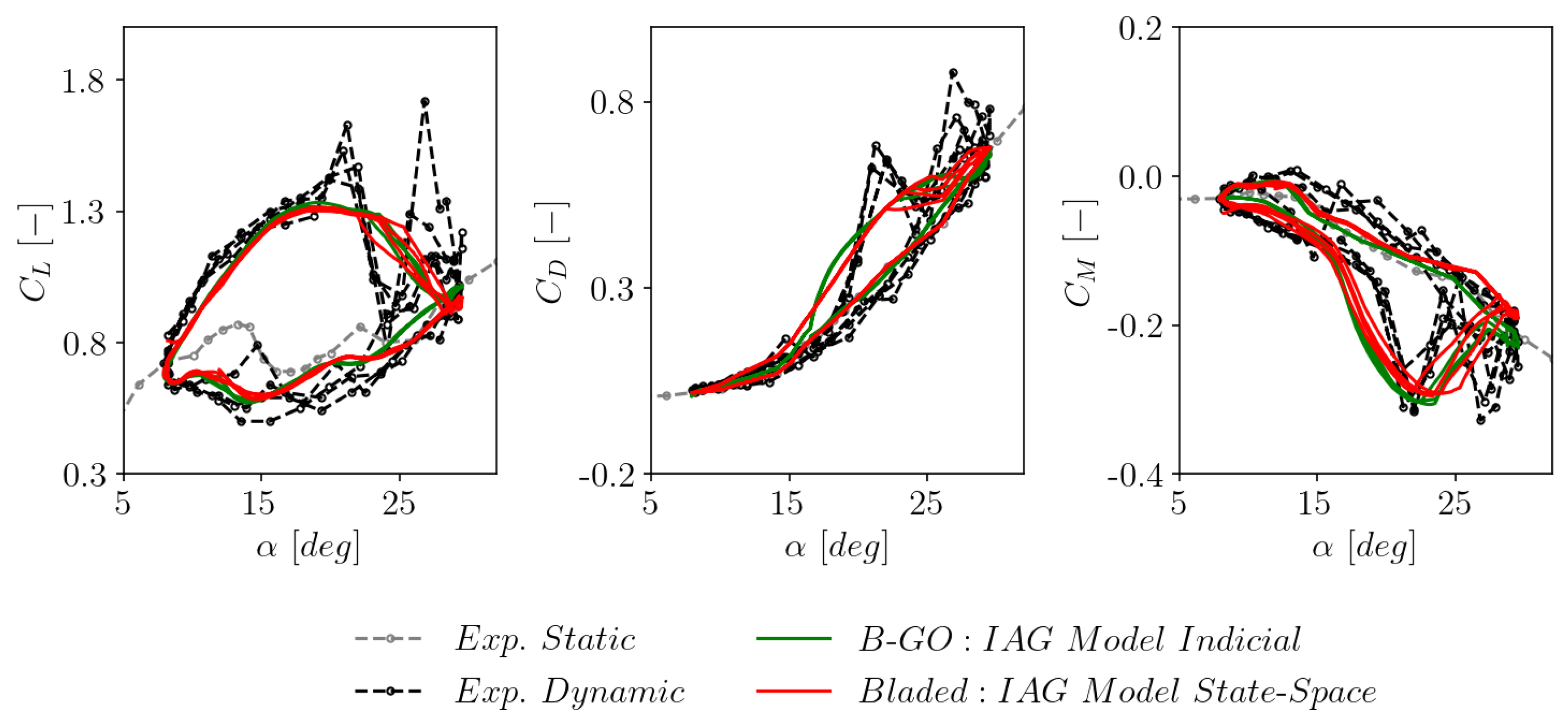
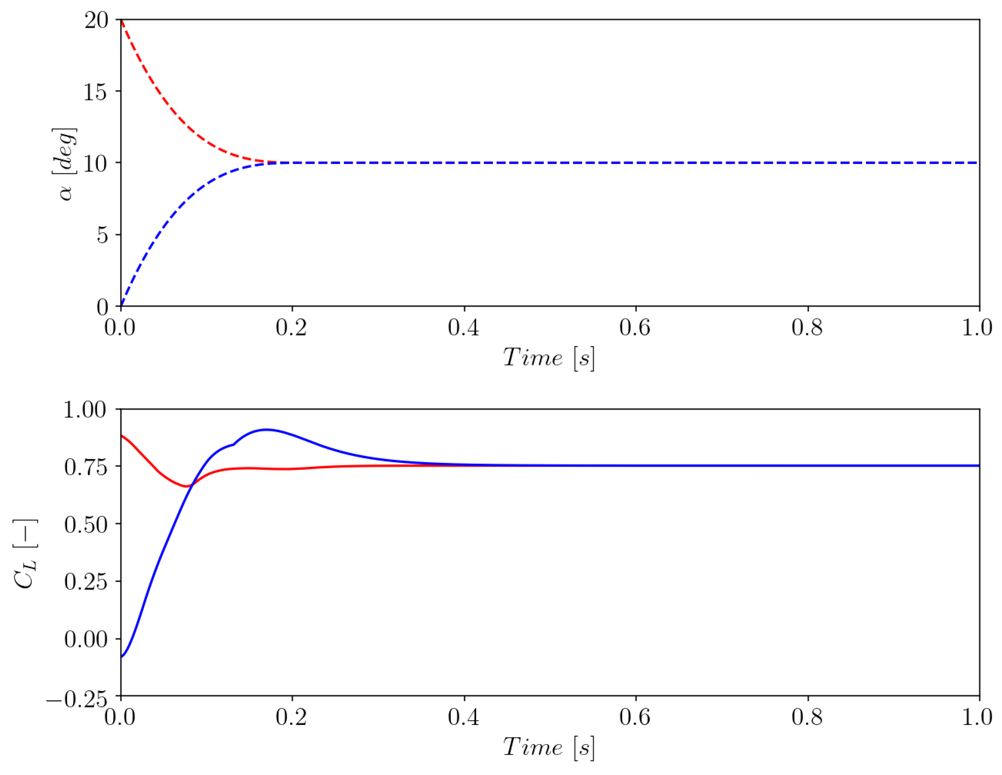
3.2. Consistency with the Original Indicial Formulation

To evaluate the consistency of the newly implemented IAG dynamic stall model in Bladed, a comparison against the original indicial formulation in the B-GO code [15,32,33] is carried out. The results of the dynamic stall calculations in Bladed using the state-space version of the IAG model are presented in Figure 4. It can be seen that the implemented state-space model using the original constant shows a reasonable consistency with the original model. Some deviations are observed especially near the maximum angle of attack. This is mainly caused by the way the critical angle of attack is defined in both models. In the newly implemented model, this is automatically determined based on the maximum normal force location, while for the original model it was observed manually at a location where the pitching moment breaks (pitching moment stall). Furthermore, the critical normal force in the indicial formulation is defined as the “inviscid” normal force based on the critical angle of attack itself. This is different with the present implementation which uses the maximum “viscous” normal force directly obtained from the polar data. When the critical normal force in B-GO is set to use the maximum viscous normal force, the agreement between both codes is significantly improved as shown in Figure 5.

Another minor source of discrepancy is the linear assumption of the attached flow polar reconstruction of the original model against sinusoidal assumption used in the present implementation. Drag deviation is a direct consequence for the normal force modeling. As for the pitching moment, no circulatory pitching moment model as in Equation (32) is used in the state-space formulation. This term is replaced with the added mass effect formulated using Equation (55), which yields a similar impact without having to provide two additional constants as in the original IAG model.

Nevertheless, the newly developed model is generally in a reasonable agreement with the original model as well as the experimental data. Note that the higher harmonic effects in the experimental data are not captured in both models because the second order model is not implemented. Only the first order term is the focus in the present studies since this term governs the main shape of the hysteresis curve.

3.3. The Effects of Mean Angle of Attack

In this section, Bladed calculations employing the IAG dynamic stall model are compared against the experimental data at three different values of the mean angle of attack, as depicted in Figure 6. Bladed calculations employing the incompressible Beddoes–Leishman model and the Øye model are also presented for comparison. The constants of the other models remain at default and are documented in [28].

It can be seen that the IAG model outperforms the other available dynamic stall model in Bladed for all three different mean angles of attack, but this is especially pronounced in the deep stall conditions. The IAG model is able to predict the hysteresis effects well, not only for the lift coefficient but also for the drag coefficient and the pitching moment coefficient. Two peaks of the lift force at $\overline{\alpha }={20}^{\circ }$ are not captured by the model because these are inherently the second order effects due to vortex shedding. This is not modeled in the first order term and requires the inclusion of the second order term.

3.4. The Effects of Reduced Frequency

The verification of the IAG dynamic stall model at various reduced frequencies is given in this section. This parameter holds a very important position in dynamic stall effects because it determines the degree of unsteadiness for the case. The results are presented in Figure 7 for three different reduced frequencies: $k=0.033$, $k=0.064$ and $k=0.098$. It can be clearly seen that the IAG dynamic stall model scales well when the reduced frequency is varied, where the stronger reduced frequency creates a stronger hysteresis loop. The same behavior is observed for the experimental data which align well with the IAG dynamic stall results. In contrast, the existing dynamic stall models in Bladed (BL and Øye) fail to predict such characteristics accurately.

3.5. The Effects of Excitation Amplitude

Figure 8 presents the dynamic polar comparison between Bladed calculations and experimental data for two different excitation amplitudes ($\Delta \alpha ={5.5}^{\circ }$ and $\Delta \alpha ={10}^{\circ }$). The highest available mean angle of attack ($\overline{\alpha }={20}^{\circ }$) is selected for the investigation because the strongest dynamic stall effect is seen at the post stall region. The already implemented BL and Øye models in Bladed are observed to underestimate the dynamic hysteresis effects significantly. For $\Delta \alpha ={5.5}^{\circ }$, it is even observed that these models do not predict any force unsteadiness. This characteristic does not agree well with the experimental data, which show force hysteresis for both investigated amplitudes. The IAG model, again, shows good agreement with the experimental data for all force components. As already observed in preceding sections, the higher harmonic effects are not captured without including the second order term for vortex shedding modeling.

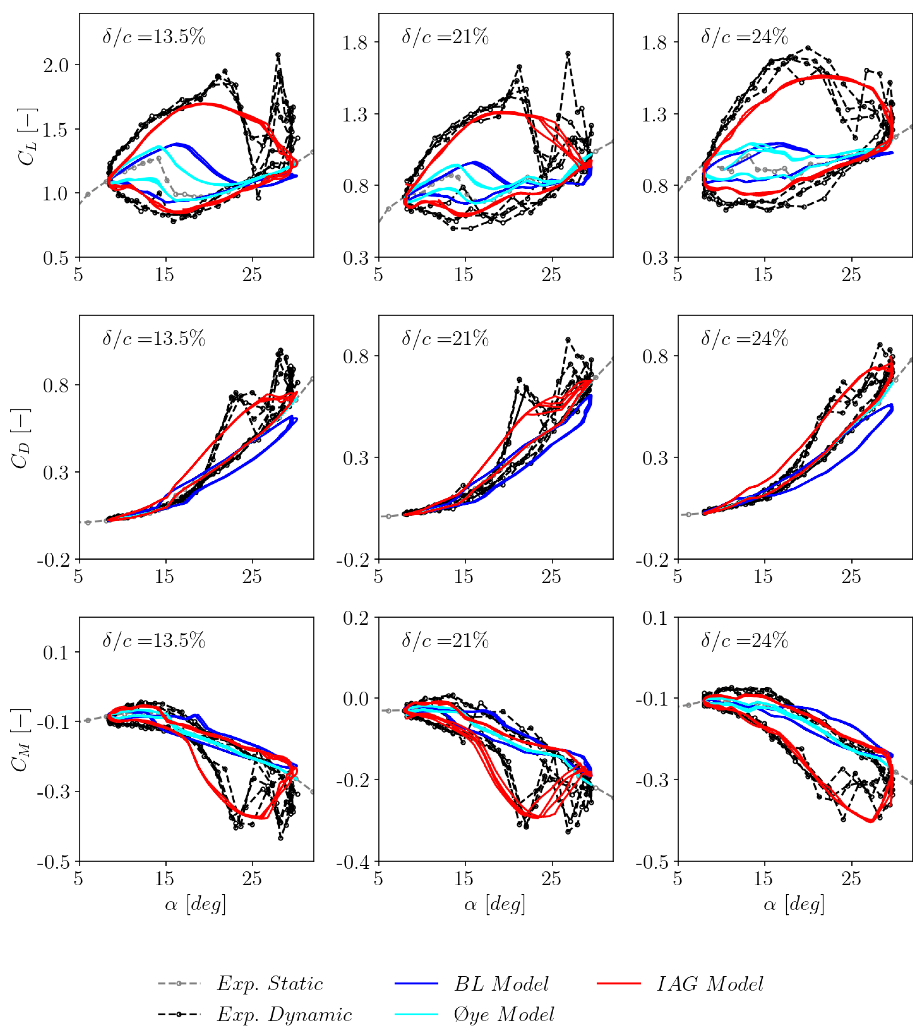
3.6. Sensitivity to Airfoil Thickness

To demonstrate the generality of the developed IAG dynamic stall model, the studies are extended to cover airfoils with different relative thicknesses. The results for all three force components are presented in Figure 9. It can be clearly seen that the airfoil thickness has a strong influence on the dynamic stall characteristics. The stall for the thinnest airfoil (S801) is the strongest among the considered airfoils in Figure 9. This is in agreement with the studies carried out in [11]. The IAG model is able to predict the stall angle location in response to the airfoil thickness to some degree. The generic shape of the polar hysteresis is predicted by the IAG model for the investigated airfoils, which clearly outperforms the BL and Øye models.

To provide a quantitative measure of how many improvements the IAG model has introduced, a quantitative measure in the form of the $L_2$ norm of error is added. The error is calculated based on:

$$\begin{array}{c}{L}_2^{\varphi }=\sqrt{\frac{1}{N}\sum _{i=1}^N{\left({\varphi }_i^{Model}-{\varphi }_i^{Exp}\right)}^2},\end{array}$$

(56)

where $\varphi$ represents the desired variable ($C_L$, $C_D$, $C_M$) calculated from the dynamic stall modeling against the experimental data. The sampling (i) is carried out for all the time series data points (N). The calculated errors for three different airfoils are presented in

Table 3. Quantified $L_2$ norm of error of three different airfoils. Measures are taken for three different aerodynamic parameters $C_L$, $C_D$ and $C_M$.

Parameter/Model	BL Model	Øye Model	IAG Model
S801 Airfoil
$C_L$	0.333	0.335	0.179
$C_D$	0.174	0.117	0.080
$C_M$	0.084	0.064	0.049
S809 Airfoil
$C_L$	0.257	0.249	0.127
$C_D$	0.133	0.084	0.057
$C_M$	0.068	0.050	0.038
S814 Airfoil
$C_L$	0.306	0.300	0.127
$C_D$	0.145	0.081	0.036
$C_M$	0.079	0.056	0.030

. It can be seen that the magnitude of the errors for all three aerodynamic properties decrease when using the IAG model regardless of the airfoil relative thickness. A similar observation is found for other parts of the studies in this paper.

3.7. Model Performance for Negative Stall

In the real operation, wind turbine airfoil sections are exposed not only to positive angle of attack regimes but also negative regimes. This is especially true when the turbine is operating in stand-still conditions at a large yaw misalignment on top of strong inflow turbulence. In this section, the performance of the IAG model in negative stall prediction will be examined. To be able to do so, negative polar data need to be generated because the OSU experimental campaign only covers the positive stall regimes. The available static and dynamic polar data sets are transformed into the negative data by applying Equation (57) to Equation (60). The synthesized static negative polar for the S809 airfoil is displayed in Figure 10.

$$\begin{array}{c}{\alpha }^{Neg}=-\alpha +2{\alpha }^{CL=0}\end{array}$$

(57)

$$\begin{array}{c}{C}_L^{Neg}=-C_L\end{array}$$

(58)

$$\begin{array}{c}{C}_D^{Neg}=C_D\end{array}$$

(59)

$$\begin{array}{c}{C}_M^{Neg}=-C_M+2C_M^{CL=0}\end{array}$$

(60)

Using the reconstructed negative data, Bladed calculations were carried out by adopting the IAG, BL and Øye models. Two mean angles of attack were considered in the simulations, having $k=0.064$, $\Delta \alpha ={10}^{\circ }$ and $Re=0.75\times {10}^6$. In Figure 11, it is demonstrated that the IAG dynamic stall model implemented in Bladed consistently shows a reasonable agreement with the experimental data, similar to its positive stall prediction accuracy. This highlights that the model is applicable both for positive and negative polar regimes. The mathematical foundation presented in Section 2.2 covers the negative stall implementation strategy and all assumptions made, allowing a full data reproduction for future follow up studies.

3.8. Sensitivity to Airfoil Surface Roughness

Investigations presented in preceding sections were done for the airfoil equipped with a surface roughness element (leading edge grit type) which promotes earlier flow transition. This stimulates soiled/rough conditions in real wind turbine operation due to dirt or insects. For new turbines or when the blades are cleaned, the turbine performance is usually higher because the aerodynamic characteristic of the airfoil is better. This is represented by “clean” airfoil measured data in Figure 12. It can be seen that the maximum lift value is higher and the stall angle of attack is slightly delayed.

To assess the performance of Bladed dynamic stall modeling under clean conditions, studies were carried out by simulating the S809 airfoil data without the surface roughness effects. The results are presented in Figure 13. Three mean angles of attack were considered in the simulations, with $k=0.064$, $\Delta \alpha ={10}^{\circ }$ and $Re=0.75\times {10}^6$. Both the IAG model and the BL model show reasonable agreement with the experimental data for $\overline{\alpha }=8^{\circ }$ and $\overline{\alpha }={14}^{\circ }$. The Øye model underestimates the hysteresis effects for both mean angles of attack. When the airfoil is operating at a deep stall condition at $\overline{\alpha }={20}^{\circ }$, both the BL model and the Øye model fail to predict the hysteresis. At this condition, only the IAG model is able to reconstruct the dynamic polar reasonably well.

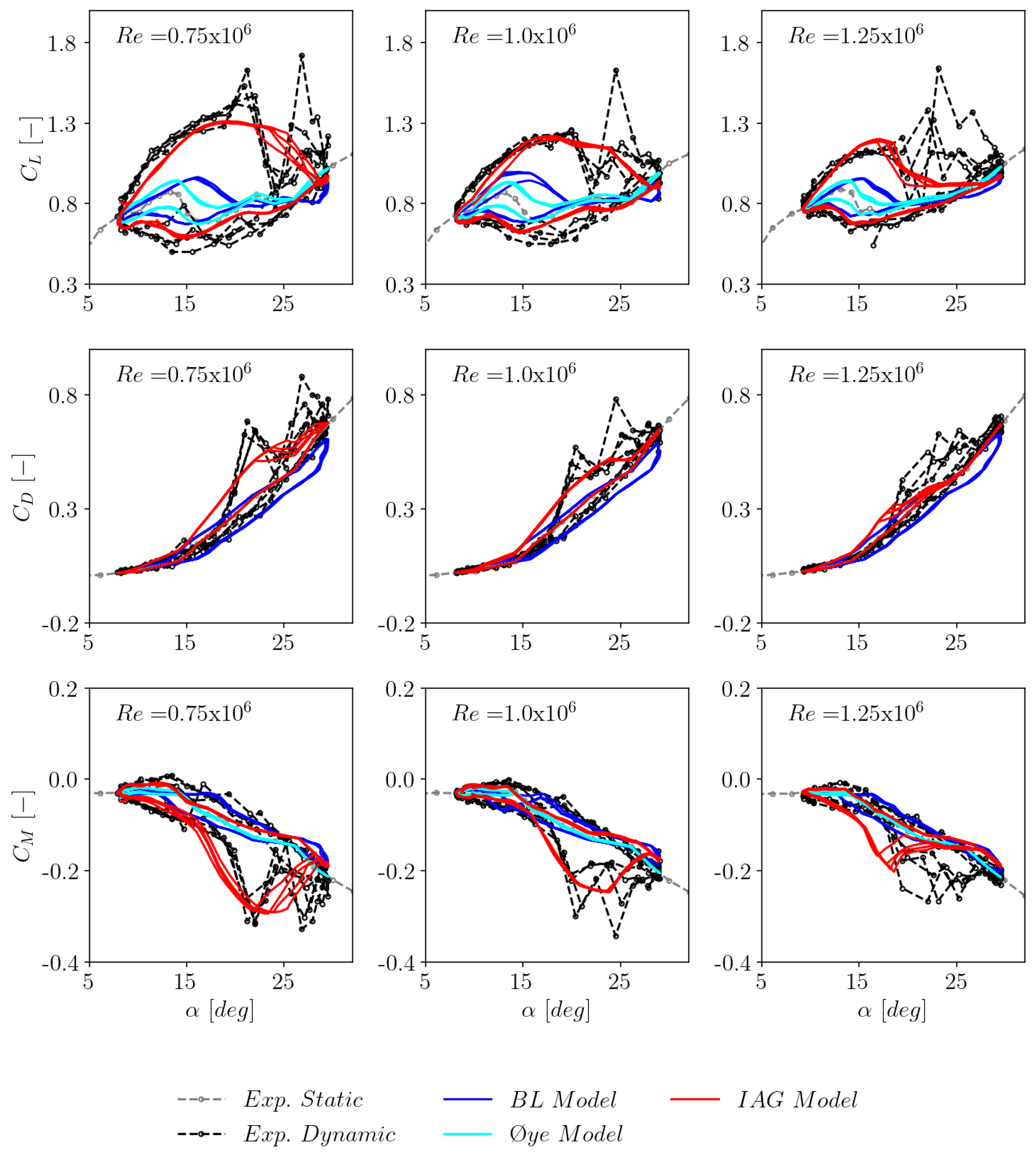
3.9. Sensitivity to Reynolds Number

The discussions are extended to cover the performance of Bladed dynamic stall modeling for three different Reynolds numbers ($Re=0.75\times {10}^6$, $Re=1.0\times {10}^6$ and $Re=1.25\times {10}^6$) in this section. The results are depicted in Figure 14. Interestingly, the effects of dynamic stall seem to scale down with increasing Reynolds number for the S809 airfoil, although the higher harmonic effects are still present for all considered Reynolds numbers. This effect is probably caused by the improved flow momentum by the increased Reynolds number. As a consequence, separation is delayed and the dynamic stall vortex is weakened. It can be seen from Figure 14 that the newly implemented IAG model is demonstrated to work and scaled well when the Reynolds number is increased.

3.10. Characteristics of Upstroke and Downstroke Motion

In most dynamic stall studies, only the unsteady excitation parameters such as the reduced frequency were usually highlighted and the transient phase where the dynamics to achieve these `quasi-stationary’ conditions were rarely discussed, e.g., how long does it take to reach stable solutions depending on initial angles of attack. An initial study of this aspect was carried out in the present paper. Figure 15 depicts the unsteady lift response predicted using the IAG model for two different initial angles of attack (different values of the initial angle of attack). The angle of attack time series is designed to converge at 0.2 s, reaching a constant value of 10${}^{\circ }$. It is worth noting that before time-domain calculations are performed, steady-state analysis is executed in Bladed to obtain the initial conditions. This is done to minimize numerical noise of the results due to initially unconverged states.

In Figure 15, it can be seen that the downstroke type motion (red curve) generally reaches the stationary condition faster than the upstroke type motion. This can be explained by the characteristics of the time delay of the dynamic stall response that is more active during the upstroke motion. This initial study shows that such an effect can hold an importance in load quantification under certain conditions, for instance short-period local wind gust. Further studies are required to explore these effects in more detail.

4. Conclusions and Outlook

Comprehensive studies have been performed in this paper to reformulate the IAG dynamic stall model into a state-space representation and to validate the results against experimental data. The implementation was carried out in the wind turbine design tool Bladed. The validations were done for various scenarios, including the effects of unsteady parameters, airfoil thickness, airfoil surface roughness and Reynolds number. The following aspects can be derived from the present paper:

• The state-space representation of the IAG model was successfully formulated.
• All the governing equations and assumptions are presented in a consistent manner to allow replication for future studies.
• The newly implemented IAG model clearly shows superior performance compared to the standard incompressible Beddoes–Leishman model and the Øye model in Bladed.
• The IAG model demonstrates a good accuracy against experimental data under various unsteady parameters, including the effects of mean angle of attack, reduced frequency and excitation amplitude.
• The IAG model results are able to be generalized to airfoils having different relative thicknesses.
• The performance of the IAG model is well validated for both clean airfoil and airfoil under the effects of surface roughness.
• The IAG model agrees well with the measurement data for three different values of the Reynolds number.
• The incompressible BL model prediction is deemed sufficient for small to moderate angle of attack cases.

The implementation of the IAG model in Bladed will allow more accurate calculations of future wind turbine load assessments. Investigations on the effects of the IAG dynamic stall model on the design load cases are highly suggested for future studies. Furthermore, dynamic stall models shall be validated for extremely high angles of attack, far beyond the static stall angle. This becomes important for wind turbine aerodynamics because the angle of attack range can reach [−180${}^{\circ }$, +180${}^{\circ }$]. It is recommended that follow up works be aimed at this aspect. The effects of initial conditions on dynamic stall can also be suggested for further exploration to fully understand the effects of short-period unsteadiness on the resulting loads. Finally, full dedicated studies on the influence of dynamic stall model on wind turbine linearization are recommended.

References

1. Bangga, G. Wind Turbine Aerodynamics Modeling Using CFD Approaches; AIP Publishing LLC: New York, NY, USA, 2022. [Google Scholar]
2. Martin, J.; Empey, R.; McCroskey, W.; Caradonna, F. An experimental analysis of dynamic stall on an oscillating airfoil. J. Am. Helicopter Soc. 1974, 19, 26–32. [Google Scholar] [CrossRef]
3. Carr, L.W.; McAlister, K.W.; McCroskey, W.J. Analysis of the Development of Dynamic Stall Based on Oscillating Airfoil Experiments; Technical Report, NASA TN D-8382; National Aeronautics and Space Administration: Washington, DC, USA, 1977. [Google Scholar]
4. McAlister, K.W.; Carr, L.W.; McCroskey, W.J. Dynamic Stall Experiments on the NACA 0012 Airfoil; Technical Report, NASA Technical Paper 1100; National Aeronautics and Space Administration: Washington, DC, USA, 1978. [Google Scholar]
5. Ramsay, R.; Hoffman, M.; Gregorek, G. Effects of Grit Roughness and Pitch Oscillations on the S801 Airfoil; Technical Report; National Renewable Energy Lab.: Golden, CO, USA, 1996. [Google Scholar]
6. Hoffman, M.; Ramsay, R.; Gregorek, G. Effects of Grit Roughness and Pitch Oscillations on the NACA 4415 Airfoil; Technical Report; National Renewable Energy Lab.: Golden, CO, USA, 1996. [Google Scholar]
7. Ramsay, R.; Hoffman, M.; Gregorek, G. Effects of Grit Roughness and Pitch Oscillations on the S809 Airfoil; Technical Report; National Renewable Energy Lab.: Golden, CO, USA, 1995. [Google Scholar]
8. Janiszewska, J.; Ramsay, R.; Hoffman, M.; Gregorek, G. Effects of Grit Roughness and Pitch Oscillations on the S814 Airfoil; Technical Report; National Renewable Energy Lab.: Golden, CO, USA, 1996. [Google Scholar]
9. Bangga, G.; Hutomo, G.; Wiranegara, R.; Sasongko, H. Numerical study on a single bladed vertical axis wind turbine under dynamic stall. J. Mech. Sci. Technol. 2017, 31, 261–267. [Google Scholar] [CrossRef]
10. Bangga, G. Numerical studies on dynamic stall characteristics of a wind turbine airfoil. J. Mech. Sci. Technol. 2019, 33, 1257–1262. [Google Scholar] [CrossRef]
11. Bangga, G.; Hutani, S.; Heramarwan, H. The Effects of Airfoil Thickness on Dynamic Stall Characteristics of High-Solidity Vertical Axis Wind Turbines. Adv. Theory Simul. 2021, 4, 2000204. [Google Scholar] [CrossRef]
12. Bangga, G. Aeroelastic Effects on Wind Turbine. In Wind Turbine Aerodynamics Modeling Using CFD Approaches; AIP Publishing LLC: Melville, NY, USA, 2022; Chapter 6; pp. 6.1–6.20. [Google Scholar]
13. Leishman, J.G.; Beddoes, T. A Semi-Empirical model for dynamic stall. J. Am. Helicopter Soc. 1989, 34, 3–17. [Google Scholar]
14. Hansen, M.H.; Gaunaa, M.; Madsen, H.A. A Beddoes–Leishman Type Dynamic Stall Model in State-Space and Indicial Formulations; Technical Report, Risø-R-1354; Risø National Laboratory: Roskilde, Denmark, 2004. [Google Scholar]
15. Bangga, G.; Lutz, T.; Arnold, M. An improved second-order dynamic stall model for wind turbine airfoils. Wind Energy Sci. 2020, 5, 1037–1058. [Google Scholar] [CrossRef]
16. Larsen, J.W.; Nielsen, S.R.; Krenk, S. Dynamic stall model for wind turbine airfoils. J. Fluids Struct. 2007, 23, 959–982. [Google Scholar] [CrossRef]
17. Gupta, S.; Leishman, J.G. Dynamic stall modeling of the S809 aerofoil and comparison with experiments. Wind Energy 2006, 9, 521–547. [Google Scholar] [CrossRef]
18. Elgammi, M.; Sant, T. A Modified Beddoes–Leishman Model for Unsteady Aerodynamic Blade Load Computations on Wind Turbine Blades. J. Sol. Energy Eng. 2016, 138, 051009. [Google Scholar] [CrossRef]
19. Wang, Q.; Zhao, Q. Modification of Leishman–Beddoes model incorporating with a new trailing-edge vortex model. Proc. Inst. Mech. Eng. Part G J. Aerosp. Eng. 2015, 229, 1606–1615. [Google Scholar] [CrossRef]
20. Sheng, W.; Galbraith, R.M.; Coton, F. A new stall-onset criterion for low speed dynamic-stall. J. Sol. Energy Eng. 2006, 128, 461–471. [Google Scholar] [CrossRef]
21. Galbraith, R. Return from Airfoil Stall During Ramp-Down Pitching Motions. J. Aircr. 2007, 44, 1856–1864. [Google Scholar]
22. Sheng, W.; Galbraith, R.; Coton, F. A modified dynamic stall model for low Mach numbers. J. Sol. Energy Eng. 2008, 130, 031013. [Google Scholar] [CrossRef]
23. Øye, S. Dynamic stall simulated as time lag of separation. In Proceedings of the 4th IEA Symposium on the Aerodynamics of Wind Turbines, Rome, Italy, 20–21 November 1990. [Google Scholar]
24. Tran, C.; Petot, D. Semi-empirical model for the dynamic stall of airfoils in view of the application to the calculation of responses of a helicopter blade in forward flight. In Proceedings of the 6th European Rotorcraft Forum, Bristol, UK, 16–19 September 1980. [Google Scholar]
25. Tarzanin, F. Prediction of control loads due to blade stall. J. Am. Helicopter Soc. 1972, 17, 33–46. [Google Scholar] [CrossRef]
26. Snel, H. Heuristic modeling of dynamic stall characteristic. In Proceedings of the European Wind Energy Conference, Dublin, Ireland, 6–9 October 1997. [Google Scholar]
27. Adema, N.; Kloosterman, M.; Schepers, G. Development of a Second Order Dynamic Stall Model. Wind Energy Sci. Discuss. 2019, 2019, 1–18. [Google Scholar] [CrossRef]
28. DNV. Bladed Theory Manual 4.14; DNV Services UK Limited: Bristol, UK, 2023. [Google Scholar]
29. Beddoes, T. Practical computation of unsteady lift. In Proceedings of the 8th European Rotorcraft Forum; 1982. Available online: http://hdl.handle.net/20.500.11881/1694 (accessed on 26 March 2023).
30. Leishman, J. Validation of approximate indicial aerodynamic functions for two-dimensional subsonic flow. J. Aircr. 1988, 25, 914–922. [Google Scholar] [CrossRef]
31. Garbaruk, A.; Shur, M.; Strelets, M.; Travin, A. NACA0021 at 60 deg. incidence. Notes Numer. Fluid Mech. Multidiscip. Des. 2009, 103, 127–139. [Google Scholar]
32. Bangga, G. Comparison of blade element method and CFD simulations of a 10 MW wind turbine. Fluids 2018, 3, 73. [Google Scholar] [CrossRef]
33. Bangga, G.; Lutz, T. Aerodynamic modeling of wind turbine loads exposed to turbulent inflow and validation with experimental data. Energy 2021, 223, 120076. [Google Scholar] [CrossRef]
Figure 1. Comparison between inviscid normal force reconstruction using a linear function, a sinusoidal function and the inviscid XFOIL data for NACA 0021.
Energies 16 03994 g001
Figure 2. Determination of the normal force gradient required for dynamic stall calculations.
Energies 16 03994 g002
Figure 3. Comparison of the measured angle of attack data points with a cubic fitted time series for the S809 airfoil at α ¯ = 20 , k = 0.064 , Δ α = 10 and R e = 0.75 × 10 6 . Variable k represents the reduced frequency ω c / ( 2 V ) .
Energies 16 03994 g003
Figure 4. Consistency between the IAG model in state-space and indicial formulations. The dynamic polar was simulated under the following conditions: α ¯ = 20 , Δ α = 10 , k = 0.064 and R e = 0.75 × 10 6 . The critical normal force in B−GO was provided as the inviscid normal force.
Energies 16 03994 g004
Figure 5. Consistency between the IAG model in state-space and indicial formulations. The dynamic polar was simulated under the following conditions: α ¯ = 20 , Δ α = 10 , k = 0.064 and R e = 0.75 × 10 6 . The critical normal force in B−GO was provided as the viscous normal force obtained directly from the polar data.
Energies 16 03994 g005
Figure 6. Dynamic polar reconstruction using Bladed for three different mean angles of attack and the comparison against measurement data. The dynamic polar was simulated under the following conditions: Δ α = 10 , k = 0.064 and R e = 0.75 × 10 6 .
Energies 16 03994 g006
Figure 7. Dynamic polar reconstruction using Bladed for three different reduced frequencies and the comparison against measurement data. The dynamic polar was simulated under the following conditions: α ¯ = 20 , Δ α = 10 and R e = 0.75 × 10 6 .
Energies 16 03994 g007
Figure 8. Dynamic polar reconstruction using Bladed for two different excitation amplitudes and the comparison against measurement data. The dynamic polar was simulated under the following conditions: α ¯ = 20 , k = 0.064 and R e = 0.75 × 10 6 .
Energies 16 03994 g008
Figure 9. Dynamic polar reconstruction using Bladed for three airfoils having different relative thicknesses and the comparison against measurement data. The dynamic polar was simulated under the following conditions: α ¯ = 20 , k = 0.064 , Δ α = 10 and R e = 0.75 × 10 6 . The considered airfoils are S801 ( δ / c = 13.5 % ), S809 ( δ / c = 21 % ) and S814 ( δ / c = 24 % ). Note that the exact value of the reduced frequency is different for each airfoil, but they are close to each other.
Energies 16 03994 g009
Figure 10. Negative polar reconstruction based on the available positive data of the S809 airfoil.
Energies 16 03994 g010
Figure 11. Dynamic polar reconstruction using Bladed for negative stall cases and comparison with measurement data. The dynamic polar was simulated under the following conditions: k = 0.064 , Δ α = 10 and R e = 0.75 × 10 6 .
Energies 16 03994 g011
Figure 12. Comparison between the clean and soiled static polar data of the S809 airfoil.
Energies 16 03994 g012
Figure 13. Dynamic polar reconstruction using Bladed for clean airfoil cases and the comparison against measurement data. The dynamic polar was simulated under the following conditions: k = 0.064 , Δ α = 10 and R e = 0.75 × 10 6 .
Energies 16 03994 g013
Figure 14. Dynamic polar reconstruction using Bladed for three different Reynolds numbers and the comparison against measurement data. The dynamic polar was simulated under the following conditions: α ¯ = 20 , k = 0.064 , Δ α = 10 . The considered Reynolds numbers are: 0.75 × 10 6 , 1.0 × 10 6 and 1.25 × 10 6 .
Energies 16 03994 g014
Figure 15. Unsteady response of S809 airfoil predicted using the IAG model for two different initial conditions. Red: downstroke, blue: upstroke.
Energies 16 03994 g015