Abstract
Operation strategies for a park-level integrated energy system (PIES) in terms of carbon prices and feed-in tariffs, have not been adequately studied. This paper addresses this knowledge gap by proposing operation strategies based on the PIES driven by biogas, solar energy, natural gas, and the power grid. Meanwhile, the electricity-driven dispatching strategy (EDS), thermal-driven dispatching strategy (TDS), cost-driven dispatching strategy (CDS) are compared to assess their impacts on operation cost, carbon dioxide emissions, etc. The flexibility and complementarity of the three operation strategies in energy supply are analyzed in detail. The results indicated that biogas was the main energy supply fuel, accounting for 46% to 72% of the total energy supply. About 33% to 54% of electricity was transmitted to the grid each month using the TDS. The annual initial capital cost of the CDS was only 1.39% higher than that of the EDS. However, the annual operation cost of the EDS was 16.86% higher than that of the CDS. The emissions of the EDS were the lowest, and the CDS had 38.51% higher emissions than the EDS. In the CDS, the ratio of carbon emission costs to operation costs was as high as 0.80 when the carbon tax reached USD 100/ton. The carbon tax had a greater impact on the CDS than the other strategies. Feed-in tariffs had a greater impact than the carbon tax on the TDS. This study provides an effective method for the selection of optimal operation strategies in regards to carbon prices and feed-in tariffs.
1. Introduction
A park-level integrated energy system (PIES) is an important strategy to achieve renewable energy consumption and carbon reduction [1]. Past research on PIESs mainly focused on system design and operation strategies. Reasonable configuration of the equipment and coordinated optimization of the operation strategies can significantly improve the utilization rate of energy and reduce costs [2]. Therefore, reasonable design and flexible operation strategies are necessary to maintain the stability and economy of a PIES.
The optimal design of a PIES involves arranging the type and capacity of the equipment before project implementation [3,4]. The operation strategy, affecting whether a PIES can perform to its designed potential, is another key factor. The most commonly used strategies are the electricity-driven dispatching strategy (EDS) and thermal-driven dispatching strategy (TDS) [5]. The EDS is known as the electricity-led strategy or electric demand management; similarly, the TDS is known as the heat-led strategy or thermal demand management [6]. However, both operation strategies have the disadvantage of generating excess heat or electricity because the energy demand constantly changes with the seasons and there is no fixed thermoelectric ratio.
Previous studies have improved operation strategies to better match the PIES. Mago et al. [7] proposed the PIES following a hybrid electric-thermal load (FHL), which has better performance compared to the EDS and TDS in terms of operation cost and carbon dioxide emissions. Zheng et al. [8] proposed an operation strategy for the PIES based on minimum distance, which has better matching performance compared with the EDS, TDS and FHL strategies. Afzali et al. [9] proposed a novel performance curve strategy based on power generation unit operating ranges for energy loads above and below the PIES operating curve. Zhao et al. [10] proposed a following operation cost strategy to determine the minimum operation cost. In addition, a mathematical model is an effective tool for the optimal configuration of the PIES. Linear programming (LP) [11], mixed-integer linear programming (MILP) [12], mixed-integer nonlinear programming (MINLP) [13], and multi-objective programming (MOP) [14] are extensively used in system optimization.
A sound evaluation of the design and operation of a PIES is also worth studying in depth. Generally, evaluation indices are considered from three aspects: total cost, primary energy consumption, and carbon dioxide emissions. Cho et al. [15] showed that there was no overall common trend among the three evaluation indices since optimizing one index might cause inverse optimization of the other two. Abdollahi et al. [16] presented a multiobjective optimization of a small-scale PIES in terms of the exergetic efficiency, total levelized cost rate of the system product, and the cost rate of the environment. Boyaghchi et al. [17] proposed a novel PIES combined with an organic Rankine cycle (ORC); the system was optimized with three objective functions of total product cost rate, exergy efficiency, and thermal efficiency. Qian et al. [18] proposed a wind-solar PIES and introduced exergy theory to evaluate the economics and sustainability.
Among all evaluation indices, CO2 emissions are receiving increasing attention. Carbon trading and carbon taxes are the two most common carbon emission reduction tools used by governments [19]. A carbon tax is a price-oriented policy tool introduced by national governments that is relatively fixed and inflexible. Several studies have examined the impact of carbon tax on PIES. Ref. [20] showed that the introduction of a carbon tax could accelerate the rollout of PIESs. When the carbon tax reached USD 25/ton, the PIES became a good choice for the energy supply system. Zeng et al. [21] proposed an off-design optimization model of a PIES-GSHP (ground source heat pump) system when considering a carbon tax. Therefore, to achieve the goal of carbon neutrality, carbon should be considered as a financial product in the design and operation of the PIES [22]. Meanwhile, since PIESs can transmit electricity to the local grid, the impact of feed-in tariffs on system operations should also be further investigated.
The sludge treatment methods of a sewage treatment plant (SWTP) include dry incineration, sanitary landfill of sludge, fertilizer, etc. However, there are few studies on the anaerobic fermentation of sludge to generate biogas and the use of biogas as fuel to provide energy for the SWTP. The stable daily sewage treatment capacity of the SWTP can produce a stable biogas supply. It is possible to build a PIES in the SWTP. However, there are few studies on the integrated energy system for the SWTP. This paper presents a PIES which uses biogas produced by anaerobic fermentation of sewage as the main fuel. This system can provide sewage treatment plant production and domestic energy. The contributions of this paper are summarized as follows: (1) An optimization model of biogas-based PIES is proposed, including initialization input, optimization method, multi-performance analysis, and final decision. (2) A CDS including the complementary characteristics of biogas, solar energy, natural gas, and power grid is proposed. (3) A comparison of the operation costs of CDS, EDS, and TDS in terms of a carbon tax and feed-in tariffs.
2. Methodology
2.1. System Description
As shown in Figure 1a, Burno et al. [23] studied a biogas production system built in an SWTP. The system had two anaerobic digesters with biogas production of 2500 Nm3/day. The same techniques and models are used in this paper. Anaerobic digesters treat sewage and continuously produce biogas. Biogas will be preferred by the PIES because it is not suitable for long-term storage due to its large storage space. Thus, PIES operation strategies should be designed to use as much biogas as possible [24]. In addition, natural gas replaces biogas for power generation and heating when biogas is scarce. The waste heat collected by the heat recovery system or the heat from the gas-fired boiler maintains the necessary temperature for biogas fermentation.
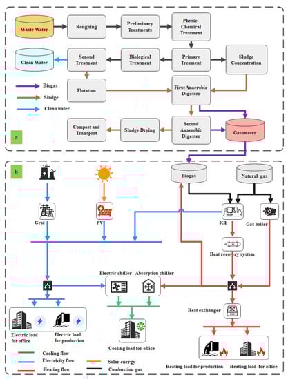
Figure 1.
Schematic configuration of the PIES system in the SWTP. (a) shows the process of producing biogas. (b) shows the diagram of the PIES.
The heat required for the anaerobic digesters is composed of three parts. The first part is the heat required to raise the temperature of the digesters to the optimum fermentation temperature. The second part is the heat loss at the boundaries of the digesters. The third part is the heat loss from the inlet and outlet pipes. The heat required for the biogas generation process in the anaerobic digesters can be expressed as follows:
where is the heat required to raise the sludge from the inlet temperature to the fermentation temperature and is the heat loss at the boundaries of digesters. Through the insulation measures, the heat loss of the pipelines () is relatively small and can be ignored. and can be expressed as follows:
where , , and represent heat loss through the base, wall, and roof, respectively. , , and represent the heat transfer coefficient of the base, wall, and roof, respectively. , , and represent the areas of the base, wall, and roof, respectively. is the temperature difference between each part and the external air. The parameters of the digesters used to calculate the heat are listed in Table 1.

Table 1.
Parameters of two digesters [23].
As shown in Figure 1b, the PIES consists of an internal combustion engine (ICE) unit, a gas-fired boiler unit, a photovoltaic (PV) unit, a heat recovery unit, an absorption chiller unit, an electric chiller unit, and a heat exchanger unit. The PIES is connected to the local power grid for bidirectional transmission of the power. The PIES is built in the SWTP to fulfill the energy demand of the plant. Sludge from the SWTP passes through the anaerobic digester to produce biogas, which is the main fuel for the ICE. In this paper, the fuels for the ICE consist of biogas and natural gas. It is feasible for some companies to manufacture an ICE that can burn a mixture of biogas and natural gas, such as the MWM company in Germany [25]. Electricity is supplied by the ICE, PV, or the local grid. Then, the waste heat from the ICE is collected by the waste heat recovery system and utilized to produce cooling or heating loads in the absorption chiller or heat exchanger, respectively. The heat supplied by the gas-fired boiler operating with natural gas is complemented by waste heat recovered from the ICE. The cooling load is supplied by the electric or absorption chiller. In the SWTP, the energy demands include the energy required for the office, the electricity required for production, and the heat required to generate biogas.
2.2. Constraints on Energy Balance and Conversion
(1) Constraints on energy balance
The constraints on the energy balance mean that the PIES must satisfy the electricity, heating, and cooling demands. The equation for the electricity balance can be expressed as follows:
where and are the electricity from the grid and PV, respectively. and are the electricity generated by ICE burning natural gas and biogas, respectively. and are electricity demands of the SWPT and the electric chiller, respectively.
The equation for the heating balance can be expressed as follows:
where represents the heat from the gas-fired boiler, respectively; represents the heat into the absorption chiller; represents the heating demands; and represents the efficiency of the heat exchanger.
The equation for the cooling balance can be expressed as follows:
where and represent the coefficient of performance of the electric chiller and absorption chiller, respectively, and represents the cooling demands.
(2) Constraints on energy conversion
Photovoltaic power generation can be expressed as follows [26]:
where is the rated power of the photovoltaic system; is the power generation efficiency of the photovoltaic system; G is the solar irradiation; is the reference solar irradiance; is the temperature coefficient; T is the operating temperature of the photovoltaic cell; and is the reference temperature of the photovoltaic cells.
The ICE generates electricity () and waste heat () by consuming natural gas and biogas [27].
where is the natural gas or biogas consumed by the ICE and is the electric efficiency of the ICE. The rated electrical efficiency of the ICE using natural gas can be expressed as follows [28]:
where is the electric efficiency at the rated capacity and is the rated capacity. The relationship between the electric efficiency and the load rate of the ICE can be expressed as follows [29]:
where represents the load rate. The electrical efficiency of the ICE using biogas can be expressed as follows [30]:
The heat value of gas fuels can be written as follows:
where is the lower heating value of the fuel (MJ/Nm3) and is the volume flow rate (Nm3/h).
The boiler is used as an auxiliary equipment to supply the insufficient heating demand. can be expressed as follows:
The cooling loads generated by the electric chiller can be expressed as follows:
The absorption chiller utilizes heat energy from the heat recovery system or gas-fired boiler. The cooling loads produced by the absorption chiller can be expressed as follows:
2.3. Constraints on Operation Strategies
(1) Electricity-driven dispatching strategy
The electricity-driven dispatching strategy (EDS) uses electricity demands as a basis to determine the heat output of the system. As renewable energy sources with no CO2 emissions, solar energy and biogas are preferentially used in the PIES. The grid and natural gas are used to fill the energy supply gap. The operation status of the PIES is shown in Figure 2 [7]. When the ICE works at point A0, the electricity and heat output through energy conversion equipment are and , respectively. In this situation, the PIES operates as follows:
where Equation (15)a represents the PIES meeting the energy demands; Equation (15)b represents the PIES generating excess heat ; Equation (15)c represents the PIES system requiring extra heat ; and “” means “and”.
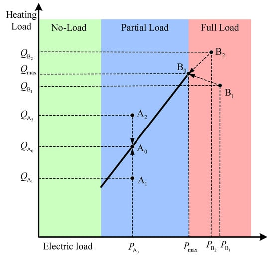
Figure 2.
Schematic diagram of the EDS.
When the PIES operates under full load conditions (point B0), the electricity and heat output through the energy conversion equipment are and , respectively. At this moment, the PIES functions as follows:
where Equation (16)a represents the PIES meeting the energy demands; Equation (16)b represents the PIES generating excess heat ; and Equation (16)c represents the PIES requiring extra heat .
(2) Thermal-driven dispatching strategy
The thermal-driven dispatching strategy (TDS) is an operation strategy that uses heat demands as a basis to determine the electricity output of the PIES. The TDS prioritizes meeting heat demands through heat recovered from the ICE and gas-fired boiler. The operation state of the ICE is shown in Figure 3 [7]. If the heat demand is too small to meet the minimum start-up conditions of the ICE, the heat is supplied by the gas-fired boiler. When the ICE works at point A0, the electricity and heat output through the various energy conversion equipment are and , respectively. In this situation, the PIES operates as follows:
where Equation (17)a exactly meets the energy demands; Equation (17)b requires additional electricity , which is supplied by the grid; and Equation (17)c transfers surplus electricity to the grid. When the ICE operates at the full load condition (point B0), the electricity and heat output through the various energy conversion equipment are and , respectively. In this situation, the PIES operates as follows:
where Equation (18)a exactly meets the energy demands; Equation (18)b requires additional electricity , which is supplied by the grid; and Equation (18)c transfers surplus electricity to the grid.
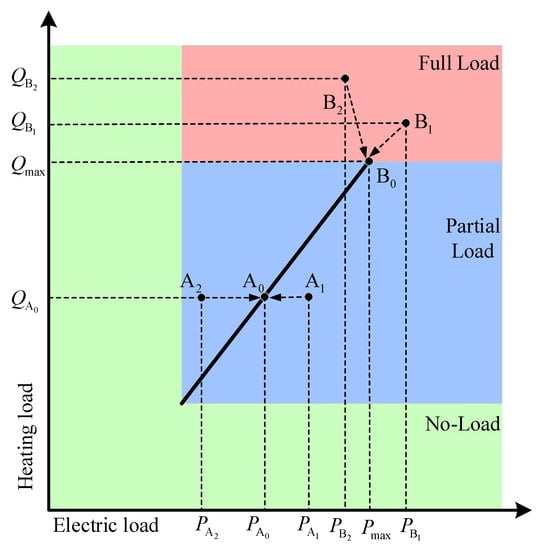
Figure 3.
Schematic diagram of the TDS.
(3) Cost-driven dispatching strategy
The cost-driven dispatching strategy (CDS) is a more flexible operation strategy than the traditional EDS and TDS. The purpose of the CDS is to minimize the operation cost of the PIES. This strategy selects the best operation mode to meet the energy demands with the optimization objective of minimizing the operation costs. The theoretical and practical basis for CDS realization is based on the time-of-use pricing service, which leads to a discrepancy between the cost of electricity purchased by the grid and the cost of generation by the ICE. The advantage of this strategy is not only to reduce the cost of electricity generation but also to ensure a sustainable and reliable electricity supply by inducing consumers to use less electricity during peak periods. The operation state of the ICE is shown in Figure 4. The price of electricity in one day is divided into three levels: peak load tariff, flat load tariff, and valley load tariff. In this situation, the PIES operates as follows:
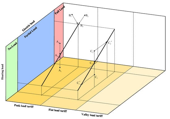
Figure 4.
Schematic diagram of the CDS.
- (1)
- If and → and .
- (2)
- If and , it will have two options: option I, the ICE operates to point C0, and the excess heat is evacuated or option II, the ICE operates to point , and the grid supplies the shortage of electricity. The algorithm will compare the cost of the two options and choose the lower-cost strategy.
- (3)
- If and , it will also have two options: option I, the ICE operates to point C0, and insufficient heat is supplied by the gas-fired boiler or option II, the ICE operates to point , and the additional electricity is transferred to the grid. The algorithm will compare the cost of the two options and choose the lower-cost strategy.
2.4. Objective Function
The comprehensive performance of the PIES depends on the design and operation strategy. With the trend of carbon neutrality, the impact of carbon emissions on the operation strategy should be considered. At the same time, the system is connected to the local grid, so the impact of feed-in tariffs on the operation strategy should also be addressed. This section presents a reasonable objective function that incorporates carbon emissions and feed-in tariffs into the evaluation index.
The objective function of the optimization model is the annual total cost (ATC), which consists of annual initial capital cost (AIPC), annual operation cost (AOC), annual maintenance cost (AMC), and annual carbon tax cost (ACC) [31]. ATC can be calculated as follows:
The AIPC can be expressed as follows:
where R is the capital recovery factor; N is the facility capacity; C is the unit price of the facility; and n is the number of facilities. The capital recovery factor R is calculated as follows:
where i and n are the interest rate (4.9%) and the service life (20 years), respectively [32].
AOC, which consists of annual electricity and natural gas costs, can be calculated as follows:
where is the annual consumption of natural gas; is the price of natural gas; is the electricity purchase price; and is the feed-in tariff. AMC is a proportion of the annual capital cost, and this study selected a value of 6% [33].
The sources of carbon dioxide emissions (CDE) in the PIES are the grid and natural gas. CDE can be expressed as follows:
where and are the CO2 emission factors of the grid and natural gas, respectively. Therefore, the annual carbon tax cost (ACC) can be expressed as follows:
where is the carbon tax. The necessary parameters are presented in Table 2 and Table 3.
Table 2.
Related parameters in the system [10,24,34,35].
Table 3.
Unit cost of the equipment in the system [23,27,35,36,37,38].
3. Case Setup
The following assumptions are made to simplify the model of the PIES and obtain the general operating characteristics of the system [23,38,39,40]: (1) the biogas yield is assumed to be determined only by the digester temperature; (2) the heat exchanger is adiabatic; (3) the composition of natural gas is CH4 (91%) and C2H6 (9%); (4) the composition of biogas is CH4 (65%) and CO2 (35%); (5) the LHV of CH4 is 35.9 MJ/Nm3; and (6) heat losses from connecting pipes are not considered.
The electric loads and heating loads of the SWTP come from the office building and the wastewater treatment process. Cooling loads in the SWTP generally come from the office building. However, the electricity required for the wastewater treatment process in SWTPs is difficult to obtain by software simulation. The same production process of SWTPs in Ref. [23] was used in this study. Therefore, the average monthly production electricity load in this study can be obtained. The heat required for biogas fermentation can be found in Section 2. The monthly average heating loads for the anaerobic digesters are shown in Figure 5. Hourly electric, heating, and cooling loads in the SWTP are presented in Figure 6. Table 4 shows the optimization results of equipment capacity.
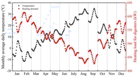
Figure 5.
Monthly average heating demands for the anaerobic digesters.
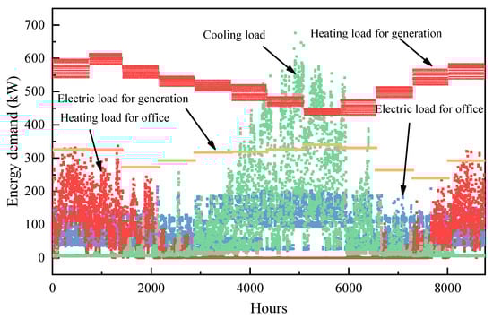
Figure 6.
Hourly electric, heating, and cooling loads in the SWTP.
Table 4.
Optimization results of equipment capacity.
4. Results and Discussion
4.1. Analysis of Operation Strategies
The hourly supply and demand of electric, heating and cooling loads are shown in this section to illustrate the operation status of the CDS, EDS, and TDS. The energy demands in summer include electric, heating, and cooling loads. The energy demands in summer include electric and heating loads. A typical day in each season is chosen to analyze the operation strategies. Figure 7 and Figure 8 present different operation strategies of the PIES on typical days. The top half of each figure is the hourly energy supply composition, and the bottom half is the hourly energy demand composition. The red line represents the time of use pricing for the grid for one day, where the peak load tariff is USD 0.1784/kWh, the flat load tariff is USD 0.1033/kWh, and the valley load tariff is USD 0.0356/kWh.
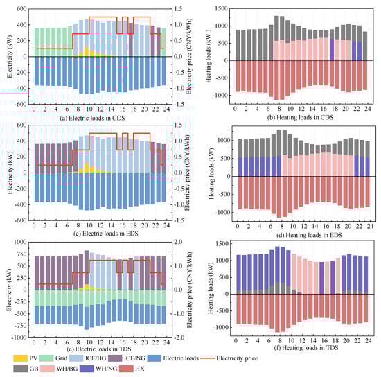
Figure 7.
Operation strategies of the PIES in winter. (a) Electric loads in CDS. (b) Heating loads in CDS. (c) Electric loads in EDS. (d) Heating loads in EDS. (e) Electric loads in TDS. (f) Heating loads in TDS. Notes: ICE/BG is the ICE driven by biogas; ICE/NG is the ICE driven by natural gas; WH/BG is the heat recovered by the waste heat recover system that is supplied by biogas; WH/NG is the heat recovered by the waste heat recover system that is supplied by natural gas; GB is the gas-fired boiler; HX is the heat exchanger. USD 1 = CNY 7.
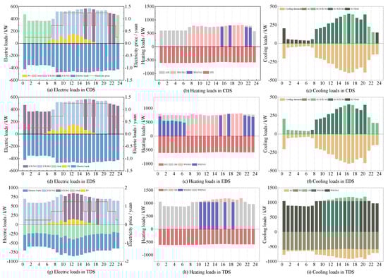
Figure 8.
CDS of the PIES in summer. (a) Electric loads in CDS. (b) Heating loads in CDS. (c) Cooling loads in CDS. (d) Electric loads in EDS. (e) Heating loads in EDS. (f) Cooling loads in EDS. (g) Electric loads in TDS. (h) Heating loads in TDS. (i) Cooling loads in TDS.
4.1.1. Winter
Figure 7 shows the CDS strategy of the PIES in winter. The PV market is growing rapidly. The aim is to increase energy independence while reducing harmful environmental impacts [41]. The combination of the three operation strategies is used by PVs to supply electricity. The hourly operation strategy was as follows:
(1) Peak load tariff (from 10:00 to 15:00, 16:00 to 17:00, and 18:00 to 20:00): For the CDS (Figure 7a,b), the ICE used biogas as the fuel to provide electricity. Using ICEs for generation reduced the stress on the local grid during the peak load period and minimized operation costs. The heat was supplied by the waste heat recovered from the ICE. The shortfall was supplied by the gas-fired boiler. During this period, the EDS operated in the same way as the CDS (Figure 7c,d). However, the TDS was different from them (Figure 7e,f). Since the heat demand was high in this period, the amount of biogas consumed per hour in the TDS was greater than that in the EDS and CDS. Biogas was exhausted at 19:00. Therefore, natural gas was needed in the remaining time. Meanwhile, the TDS generated surplus electricity, which was sold to the local grid. Therefore, the economics of the TDS were influenced by the feed-in tariff.
(2) Flat load tariff (from 7:00 to 10:00, 15:00 to 16:00, 17:00 to 18:00, and 21:00 to 23:00): For the CDS, the ICE used biogas to generate electricity in the first few hours. When biogas was insufficient, natural gas was used as fuel. For example, from 17:00 to 18:00 and 21:00 to 23:00, the ICE used natural gas to supply electricity when the ICE had an advantage over the grid in terms of operation cost and carbon dioxide emissions. The source of the waste heat recovered from the ICE during these hours was natural gas. The EDS operates in a similar way to the CDS in this period. As biogas was used up during the peak load period, the TDS used natural gas to drive the ICE to produce electricity and heat (Figure 7f). Surplus electricity was sold to the local grid. Insufficient heat was supplied by the boiler.
(3) Valley load tariff (from 23:00 to 7:00): During this time period, grid electricity was the cheapest. Therefore, the CDS supplied electricity from the grid at these times (Figure 7a). Since the ICE did not start, the heat was supplied by the gas-fired boiler, as shown in Figure 7b. The EDS and TDS chose the ICE to supply electricity and heat due to a balance of heat requirements. The electricity and heat beyond the rated capacity of the ICE were supplied by the grid and gas-fired boiler, respectively.
4.1.2. Summer
Figure 8 showed the different strategies of the PIES in summer. The hourly operation strategy was as follows:
(1) Peak load tariff (from 10:00 to 15:00, 16:00 to 17:00, and 18:00 to 20:00): For electric and heating loads, the operation details of the three strategies were similar to those in winter. For the CDS and EDS, all the cooling loads during this period were supplied by the electric chiller, and the electricity required to make the electric chiller work comes from the electricity generated by the ICE consuming biogas. For the TDS, cooling loads were supplied by the absorption chiller.
(2) Flat load tariff (from 7:00 to 10:00, 15:00 to 16:00, 17:00 to 18:00, and 21:00 to 23:00): For the CDS and EDS, cooling loads were supplied by the electric chiller. The electricity required to make the electric chiller function comes from the electricity generated by the ICE. For the CDS, the electricity supplied by the ICE could not fully meet the demands of the electric chiller. Therefore, the cooling loads generated by the electric chiller were not enough to meet the cooling demand. Insufficient cooling loads were supplied by the absorption chiller. For the TDS, the cooling loads were also supplied by the absorption chiller.
(3) Valley load tariff (from 23:00 to 7:00): For the CDS, the electricity required for the operation of the electric chiller was supplied by the grid. For the EDS, the electricity required for the electric chiller was supplied by the ICE. For the TDS, the cooling loads were supplied by the absorption chiller. These were related to the logic of the operation strategies and coordinated with the modes of heating and electric supply.
4.1.3. Performance Comparisons of Operation Strategies
Figure 9 shows the evaluation indices of the three operation strategies. The annual initial capital cost (AIPC) of the CDS was only 1.39% higher than that of the EDS. However, the annual operation cost (AOC) of the EDS was 16.86% higher than that of the CDS. These results further supported that the CDS has a greater advantage in operation costs. In this case, we selected valley load tariff as the feed-in tariff. A considerable amount of electricity was sold to the local grid company in this case. Therefore, it resulted in the highest operation cost of the TDS. The emissions of the EDS were the lowest, and the CDS had 38.51% higher emissions than the EDS. The reason for this huge gap was that the CDS purchased electricity from the local grid during the valley load period. Obviously, the CDS had advantages in operation costs and investment payback period, while the EDS had an advantage in reducing carbon dioxide emissions. Therefore, it is economically advisable to invest in specific park-level integrated energy systems because they pay off quickly [42].
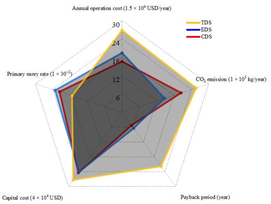
Figure 9.
Comparison of evaluation indices among the three operation strategies.
4.2. Energy Consumption
The monthly energy consumption of the CDS is shown in Figure 10. Biogas was the main energy supply fuel, accounting for 46% to 72% of the total energy supply. Biogas produced by sludge fermentation has been comprehensively utilized. The transition to a low-carbon energy system is one of the world’s main priorities. A precondition for this transition is to increase the share of renewable energy sources in the energy system [43]. Therefore, the system proposed in this paper is in line with the development trend of energy. The second largest energy supply came from the local power grid, accounting for 18% to 31% of the total energy supply. The photovoltaic output power was mainly determined by solar irradiance. Natural gas was used as a type of supplementary energy. Biogas, photovoltaics, and the grid can guarantee electricity demand during months when the demand for electricity was low. There was no need to consume natural gas to supply electricity, in months such as March, April, October, November, and December. The more electricity that was needed, the more natural gas that was needed to be used. For example, from May to August, the electric loads increased monthly, and the percentage of natural gas Increased from 4% to 20%. This optimization result was reasonable from the perspective of minimizing operation costs. The monthly energy consumption of the EDS is shown in Figure 11. The main fuel for power generation was biogas, which accounted for 43% to 75% of the total energy supply. The monthly energy consumption of the TDS is shown in Figure 12. About 33% to 54% of the electricity was transmitted to the grid each month, so the cost of the TDS was influenced by the feed-in tariffs.
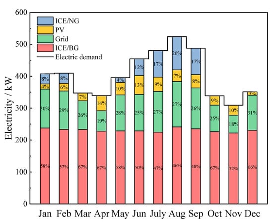
Figure 10.
Composition of the fuel consumption in the CDS.
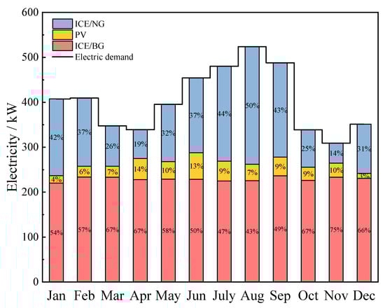
Figure 11.
Composition of the fuel consumption in the EDS.
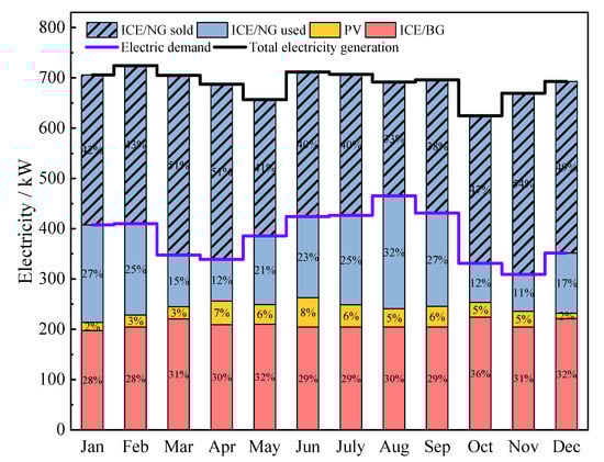
Figure 12.
Composition of the fuel consumption in the TDS.
4.3. Sensitivity Analysis of Carbon Taxes and Feed-In Tariffs
Figure 13 shows the ratio of carbon costs to operation costs in the CDS, EDS, and TDS. Figure 13d shows the impact of feed-in tariffs on operation costs in the TDS. The carbon prices had the greatest influence on the CDS, and the ratio of carbon emission costs to operation costs was as high as 0.90 when the carbon price reached USD 100/ton. Compared with the CDS, this ratio was approximately 0.50 in the EDS and 0.60 in the TDS. April and November in the CDS were less affected by the carbon price because they emitted the least amount of CO2 during the year. As shown in Figure 10, only 19% of electricity was supplied by the grid in April and 18% in November. The impact of feed-in tariffs on the TDS was greater than that of carbon tax by comparing Figure 13c,d. Figure 12 shows that in August, only 33% of the total electricity generated was sent to the grid. April and November were more affected by feed-in tariffs because the TDS generated the maximum amount of electricity in these two months of the year.
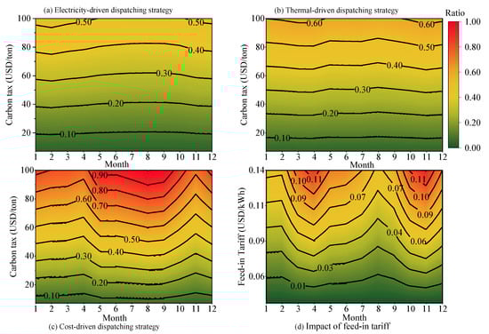
Figure 13.
Impact of carbon price and feed-in tariffs on monthly operation costs. (a) Impact of carbon prices on the ratio of carbon emission costs to monthly operating costs in EDS; (b). Impact of carbon prices on the ratio of carbon emission costs to monthly operating costs in TDS; (c). Impact of carbon prices on the ratio of carbon emission costs to monthly operation costs in CDS; (d). Impact of feed-in tariffs on the ratio of the revenue through electricity sales to monthly operation costs in TDS.
Figure 14 shows the impact of carbon price on operation strategies in the range of USD 0 to 100/ton. Points A, B, C, D, and E were critical points, which showed the carbon price when the annual total costs of the strategies were equivalent. When the feed-in tariff was FIT1 and the carbon price ranged from CA to CC, the total cost of the CDS was the lowest, i.e., line segment AC. When the feed-in tariff was FIT1 and the carbon price ranged from c to e, the total cost of the EDS was the lowest, i.e., line segment CE. When the feed-in tariff was FIT2 and the carbon price ranged from CA to CB, the total cost of the TDS was the lowest, i.e., line segment AB. When the feed-in tariff was FIT2 and the carbon price was from CB to CC, the total cost of the CDS was the lowest, i.e., line segment BC. When the feed-in tariff was FIT2 and the carbon price ranged from CC to CE, the total cost of the TDS was the lowest, i.e., line segment CE. When the feed-in tariff was FIT3 and the carbon price ranged from CA to CD, the total cost of the TDS was the lowest, i.e., line segment AD. When the feed-in tariff was FIT3 and the carbon price was from CD to CE, the total cost of the EDS was the lowest, i.e., line segment DE. When the feed-in tariff was FIT4 and the carbon price ranged from CA to CE, the total cost of the TDS was the lowest, i.e., line segment AE.
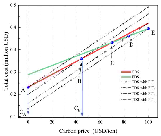
Figure 14.
Total cost of the CDS, EDS, and TDS in terms of carbon prices and feed-in tariffs. Notes: FIT1 to FIT4 mean that the feed-in tariffs are USD 0.0356, 0.0642, 0.0928, and 0.1213/kWh, respectively.
Therefore, these results provide important insights into flexibly selecting the optimal operation strategy according to carbon prices and feed-in tariffs. With this approach, we have the flexibility to select the optimal operation strategy.
5. Conclusions
This study proposed a park-level integrated energy system coupled with biogas built in a sewage treatment plant. Three operation strategies were proposed: electricity-driven dispatching strategy (EDS), thermal-driven dispatching strategy (TDS), and cost-driven dispatching strategy (CDS). The effect of carbon prices and feed-in tariffs on operation costs of the park-level integrated energy system was studied by optimizing the three operation strategies. The conclusion of this paper has guiding significance for selecting the optimal operation strategy. The main conclusions are summarized as follows: (1) Biogas as the main fuel of the system was fully utilized during the period of peak load tariffs. As the supplementary fuel, the consumption of natural gas increased with the increase in energy demand. The CDS had the minimum total cost. In addition, the EDS had the lowest carbon dioxide emissions. (2) The annual initial capital cost of the CDS was only 1.39% higher than that of the EDS. However, the annual operation cost of the EDS was 16.86% higher than that of the CDS. The emissions of the EDS were the lowest, and the CDS had 38.51% higher emissions than the EDS. (3) The annual carbon cost of the cost-driven dispatching strategy accounted for the largest proportion of the total cost. When the carbon price reached USD 100/ton, the ratio of carbon cost to total cost was as high as 0.80. Fluctuations in feed-in tariffs had a greater impact on the thermal-driven dispatching strategy than carbon prices. (4) The operation costs were influenced by various factors, such as natural gas prices, electricity prices, carbon prices, and feed-in tariffs. Changes in these factors and fluctuations in energy demand would lead to a marked shift in the operation costs. Therefore, the optimal operation strategy was not fixed.
Author Contributions
Conceptualization, X.Z.; Investigation, H.C.; Methodology, X.Z.; Resources, G.X.; Writing—original draft, X.Z.; Writing—review and editing, Y.C. All authors have read and agreed to the published version of the manuscript.
Funding
This research was funded by the Major Program of the National Natural Science Foundation of China (No. 52090064).
Data Availability Statement
Not applicable.
Conflicts of Interest
No conflict of interest exist in the submission of this manuscript, and the manuscript has been approved by all authors for publication.
References
- Ju, L.W.; Tan, Z.F.; Li, H.H.; Tan, Q.K.; Yu, X.B.; Song, X.H. Multi-objective operation optimization and evaluation model for PIES and renewable energy based hybrid energy system driven by distributed energy resources in China. Energy 2016, 111, 322–340. [Google Scholar] [CrossRef]
- Li, M.; Mu, H.L.; Li, N.; Ma, B.Y. Optimal design and operation strategy for integrated evaluation of PIES (combined cooling heating and power) system. Energy 2016, 99, 202–220. [Google Scholar] [CrossRef]
- Kang, L.G.; Wu, X.J.; Yuan, X.X.; Ma, K.R.; Wang, Y.Z.; Zhao, J.; An, Q.S. Influence analysis of energy policies on comprehensive performance of PIES system in different buildings. Energy 2021, 233, 121–159. [Google Scholar] [CrossRef]
- Moussawi, H.A.; Fardoun, F.; Louahlia-Gualous, H. Review of tri-generation technologies: Design evaluation, optimization, decision-making, and selection approach. Energy Convers. Manag. 2016, 120, 157–196. [Google Scholar] [CrossRef]
- Mago, P.J.; Fumo, N.; Chamra, L.M. Performance analysis of PIES and CHP systems operating following the thermal and electric load. Int. J. Energy Res. 2009, 33, 852–864. [Google Scholar] [CrossRef]
- Smith, A.D.; Mago, P.J. Effects of load-following operational methods on combined heat and power system efficiency. Appl. Energy 2014, 115, 337–351. [Google Scholar] [CrossRef]
- Mago, P.J.; Chamra, L.M.; Ramsay, J. Micro-combined cooling, heating and power systems hybrid electric-thermal load following operation. Appl. Therm. Eng. 2010, 30, 800–806. [Google Scholar] [CrossRef]
- Zheng, C.Y.; Wu, J.Y.; Zhai, X.Q. A novel operation strategy for PIES systems based on minimum distance. Appl. Energy 2014, 128, 325–335. [Google Scholar] [CrossRef]
- Afzali, S.F.; Mahalec, V. Novel performance curves to determine optimal operation of PIES systems. Appl. Energy 2018, 226, 1009–1036. [Google Scholar] [CrossRef]
- Zhao, X.; Zheng, W.; Hou, Z.; Chen, H.; Xu, G.; Liu, W.; Chen, H.G. Economic dispatch of multi-energy system considering seasonal variation based on hybrid operation strategy. Energy 2022, 238, 121–733. [Google Scholar] [CrossRef]
- Rong, A.; Lahdelma, R. An efficient linear programming model and optimization algorithm for trigeneration. Appl. Energy 2005, 82, 40–63. [Google Scholar] [CrossRef]
- Ren, H.; Gao, W. A MILP model for integrated plan and evaluation of distributed energy systems. Appl. Energy 2010, 87, 1001–1014. [Google Scholar] [CrossRef]
- Li, H.; Nalim, R.; Haldi, P.A. Thermal-economic optimization of a distributed multi-generation energy system—A case study of Beijing. Appl. Therm. Eng. 2006, 26, 709–719. [Google Scholar] [CrossRef]
- Carvalho, M.; Lozano, M.A.; Serra, L.M. Multicriteria synthesis of trigeneration systems considering economic and environmental aspects. Appl. Energy 2012, 91, 245–254. [Google Scholar] [CrossRef]
- Cho, H.; Mago, P.J.; Luck, R.; Chamra, L.M. Evaluation of PIES systems performance based on operational cost, primary energy consumption, and carbon dioxide emission by utilizing an optimal operation scheme. Appl. Energy 2009, 86, 2540–2549. [Google Scholar] [CrossRef]
- Abdollahi, G.; Sayyaadi, H. Application of the multi-objective optimization and risk analysis for the sizing of a residential small-scale PIES system. Energy Build. 2013, 60, 330–344. [Google Scholar] [CrossRef]
- Boyaghchi, F.A.; Heidarnejad, P. Thermoeconomic assessment and multi objective optimization of a solar micro PIES based on Organic Rankine Cycle for domestic application. Energy Convers. Manag. 2015, 97, 224–234. [Google Scholar] [CrossRef]
- Qian, J.; Wu, J.; Yao, L.; Mahmut, S.; Zhang, Q. Comprehensive performance evaluation of Wind-Solar-PIES system based on emergy analysis and multi-objective decision method. Energy 2021, 230, 120–779. [Google Scholar] [CrossRef]
- Jia, Z.; Lin, B. Rethinking the choice of carbon tax and carbon trading in China. Technol. Forecast. Soc. 2020, 159, 120–187. [Google Scholar] [CrossRef]
- Zhang, L.; Gao, W.; Yang, Y.; Qian, F. Impacts of Investment Cost, Energy Prices and Carbon Tax on Promoting the Combined Cooling, Heating and Power (PIES) System of an Amusement Park Resort in Shanghai. Energies 2020, 13, 4252. [Google Scholar] [CrossRef]
- Zeng, R.; Zhang, X.; Deng, Y.; Li, H.; Zhang, G. An off-design model to optimize PIES-GSHP system considering carbon tax. Energy Convers. Manag. 2019, 189, 105–117. [Google Scholar] [CrossRef]
- Brink, C.; Vollebergh, H.R.J.; van der Werf, E. Carbon pricing in the EU: Evaluation of different EU ETS reform options. Energy Policy 2016, 97, 603–617. [Google Scholar] [CrossRef]
- Bruno, J.C.; Ortega-López, V.; Coronas, A. Integration of absorption cooling systems into micro gas turbine trigeneration systems using biogas: Case study of a sewage treatment plant. Appl. Energy 2009, 86, 837–847. [Google Scholar] [CrossRef]
- Su, B.; Han, W.; Chen, Y.; Wang, Z.; Qu, W.; Jin, H. Performance optimization of a solar assisted PIES based on biogas reforming. Energy Convers. Manag. 2018, 171, 604–617. [Google Scholar] [CrossRef]
- MWM. Available online: https://www.mwm.net/ (accessed on 8 July 2022).
- Gazda, W.; Stanek, W. Energy and environmental assessment of integrated biogas trigeneration and photovoltaic plant as more sustainable industrial system. Appl. Energy 2016, 169, 138–149. [Google Scholar] [CrossRef]
- Jia, J.; Chen, H.; Liu, H.; Ai, T.; Li, H. Thermodynamic performance analyses for PIES system coupled with organic Rankine cycle and solar thermal utilization under a novel operation strategy. Energy Convers. Manag. 2021, 239, 114212. [Google Scholar] [CrossRef]
- Kalina, J. Integrated biomass gasification combined cycle distributed generation plant with reciprocating gas engine and ORC. Appl. Therm. Eng. 2011, 31, 2829–2840. [Google Scholar] [CrossRef]
- He, X.; Cai, R. Typical off-design analytical performances of internal combustion engine cogeneration. Front. Energy Power Eng. China 2009, 3, 184–192. [Google Scholar] [CrossRef]
- Wang, J.; Sui, J.; Jin, H. An improved operation strategy of combined cooling heating and power system following electrical load. Energy 2015, 85, 654–666. [Google Scholar] [CrossRef]
- Angrisani, G.; Akisawa, A.; Marrasso, E.; Roselli, C.; Sasso, M. Performance assessment of cogeneration and trigeneration systems for small scale applications. Energy Convers. Manag. 2016, 125, 194–208. [Google Scholar] [CrossRef]
- Jiang, R.; Qin, F.G.F.; Yin, H.; Yang, M.; Xu, Y. Thermo-economic assessment and application of PIES system with dehumidification and hybrid refrigeration. Appl. Therm. Eng. 2017, 125, 928–936. [Google Scholar] [CrossRef]
- Zhang, G.; Li, Y.; Zhang, N. Performance analysis of a novel low CO2-emission solar hybrid combined cycle power system. Energy 2017, 128, 152–162. [Google Scholar] [CrossRef]
- Guo, L.; Liu, W.; Cai, J.; Hong, B.; Wang, C. A two-stage optimal planning and design method for combined cooling, heat and power microgrid system. Energy Convers. Manag. 2013, 74, 433–445. [Google Scholar] [CrossRef]
- Wang, J.; Jing, Y.; Zhang, C. Optimization of capacity and operation for PIES system by genetic algorithm. Appl. Energy 2010, 87, 1325–1335. [Google Scholar] [CrossRef]
- Wang, J.; Xu, Z.; Jin, H.; Shi, G.; Fu, C.; Yang, K. Design optimization and analysis of a biomass gasification based BCHP system: A case study in Harbin, China. Renew. Energy 2014, 71, 572–583. [Google Scholar] [CrossRef]
- Petrollese, M.; Cocco, D. Techno-economic assessment of hybrid CSP-biogas power plants. Renew. Energy 2020, 155, 420–431. [Google Scholar] [CrossRef]
- Kulkarni, M.N.K.; Patekar, M.S.; Bhoskar, M.T.; Kulkarni, M.O.; Kakandikar, G.M.; Nandedkar, V.M. Particle Swarm Optimization Applications to Mechanical Engineering- A Review. Mater. Today Proc. 2015, 2, 2631–2639. [Google Scholar] [CrossRef]
- Mehr, A.S.; Gandiglio, M.; MosayebNezhad, M.; Lanzini, A.; Mahmoudi, S.M.S.; Yari, M.; Santarelli, M. Solar-assisted integrated biogas solid oxide fuel cell (SOFC) installation in wastewater treatment plant: Energy and economic analysis. Appl. Energy 2017, 191, 620–638. [Google Scholar] [CrossRef]
- Zhang, G.; Li, Y.; Dai, Y.J.; Wang, R.Z. Design and analysis of a biogas production system utilizing residual energy for a hybrid CSP and biogas power plant. Appl. Therm. Eng. 2016, 109, 423–431. [Google Scholar] [CrossRef]
- Chomać-Pierzecka, E.; Kokiel, A.; Rogozińska-Mitrut, J.; Sobczak, A.; Soboń, D.; Stasiak, J. Analysis and Evaluation of the Photovoltaic Market in Poland and the Baltic States. Energies 2022, 15, 669. [Google Scholar] [CrossRef]
- Neacșa, A.; Panait, M.; Mureșan, J.D.; Voica, M.C.; Manta, O. The Energy Transition between Desideratum and Challenge: Are Cogeneration and Trigeneration the Best Solution? Int. J. Environ. Res. Public Health 2022, 19, 3039. [Google Scholar] [CrossRef] [PubMed]
- Sobczak, A.; Chomać-Pierzecka, E.; Kokiel, A.; Różycka, M.; Stasiak, J.; Soboń, D. Economic Conditions of Using Biodegradable Waste for Biogas Production, Using the Example of Poland and Germany. Energies 2022, 15, 5239. [Google Scholar] [CrossRef]
Disclaimer/Publisher’s Note: The statements, opinions and data contained in all publications are solely those of the individual author(s) and contributor(s) and not of MDPI and/or the editor(s). MDPI and/or the editor(s) disclaim responsibility for any injury to people or property resulting from any ideas, methods, instructions or products referred to in the content. |
© 2022 by the authors. Licensee MDPI, Basel, Switzerland. This article is an open access article distributed under the terms and conditions of the Creative Commons Attribution (CC BY) license (https://creativecommons.org/licenses/by/4.0/).