Article

Time-Series Well Performance Prediction Based on Convolutional and Long Short-Term Memory Neural Network Model

1
Jinan Bestune Times Power Technology Co., Ltd., Jinan 250000, China
2
The Second Gas Production Plant of PetroChina Changqing Oilfield Company, Yulin 719000, China
3
School of Energy, Faculty of Engineering, China University of Geosciences, Beijing 100083, China
*
Author to whom correspondence should be addressed.
Energies 2023, 16(1), 499; https://doi.org/10.3390/en16010499
Submission received: 8 December 2022 / Revised: 23 December 2022 / Accepted: 28 December 2022 / Published: 2 January 2023

Abstract

:
In the past, reservoir engineers used numerical simulation or reservoir engineering methods to predict oil production, and the accuracy of prediction depended more on the engineers’ own experience. With the development of data science, a new trend has arisen to use deep learning to predict oil production from the perspective of data. In this study, a hybrid forecasting model (CNN-LSTM) based on a convolutional neural network (CNN) and a Long Short-Term Memory (LSTM) neural network is proposed and used to predict the production of fractured horizontal wells in volcanic reservoirs. The model solves the limitation of traditional methods that rely on personal experience. First, the production constraints and production data are used to form a feature space, and the abstract semantics of the feature time series are extracted through convolutional neural network, then the LSTM neural network is used to predict the time series. The certain hyperparameters of the whole model are optimized by Particle Swarm Optimization algorithm (PSO). In order to estimate the model, some production dynamics from the Xinjiang oilfield of China are used for comparative analysis. The experimental results show that the CNN-LSTM model is superior to traditional neural networks and conventional decline curves.

1. Introduction

As an important fossil energy source, petroleum has always been considered in regard to providing oil recovery to maximize economic benefits [1]. If the oil production can be accurately predicted, it can help engineers adjust the development mode in different development stages. It is worth noting that although the oil production is a time series, the uncertainty of characteristic dimensions and the periodic adjustment of production constraints have exacerbated the nonlinearity, non-smoothness and complexity of the production forecast. For reservoir engineers, there are three common prediction methods. The first is reservoir numerical simulation. Geological modeling, dynamic parameter configuration and history matching are conducted through reservoir static data and development engineering parameters [2,3,4], and engineers often need to spend a lot of time in numerical simulation [3,4]. The second is the analytic model. The physical model is simplified into a solvable mathematical model through a series of boundary conditions and assumptions, and solved through mathematical physical equations [5,6,7]. Although it requires less time than numerical simulation, in order to describe the percolation mechanism of a specific reservoir, physical simulation experiments need to be used for theoretical support. In the third method, engineers can also use reservoir engineering methods summarized by predecessors such as decline curve analysis for time series prediction. Although this method is simple, it ignores the impact of production constraints and other well performance factors on production.
In addition to the traditional methods mentioned above, with the development of machine learning, data-driven algorithms have become a new solution to solve problems. By using multi-dimensional Kriging, gradient enhancement machine, random forest (RF) and support vector machine (SVM), Schuetter et al. [8] attempted to predict production and proposed guidelines to enhance the robustness of time-series prediction models. On this basis, subsequent research uses SVM to establish the prediction model of initial oil production. RF and SVM are applied to Wolfcamp shale reservoir in Permian basin [9,10,11,12,13]. Although the research has proved the accuracy of the prediction, this type of model is only applicable to point data prediction, ignoring the time-series nature of production rate, which means that the application scope of the model is greatly reduced and can only be used to predict recovery factor, cumulative production, initial rate and other point data. Cao et al. [14] focused on ecological dynamic factors and studied the relationship between tubing head pressure and productivity. Although the problem of characterizing productivity time series has not been solved, the tubing head pressure is a function of time, which indirectly reflects the time correlation of time series data. Because it is recorded with productivity at the same time on site, it is impossible to obtain the tubing head pressure when predicting the productivity in the field application.
With the development of deep learning, a neural network model provides new ideas for research. Many scholars try to use the artificial neural network (ANN) model to predict production. They train factors such as pressure, temperature or specific decline mode as input items, and gradually take into account the temporal correlation of characteristics [15,16]. In addition, the recurrent neural networks for natural language processing have also been introduced into the study of time-series prediction. Li et al. [17] proposed a Temporary Convolutional Network (TCN). They used this model to learn wellhead pressure data to predict productivity. Wang et al. [18] used LSTM neural network to train existing oilfield production data to predict oilfield production in ultra-high water cut stage. Considering the Arps decline model cannot meet the requirements of field application, Cheng et al. [19] used the LSTM neural network and Gate Recursive Unit (GRU) to predict oil production. Al-Shabandar et al. [20] presented a deep gated recurrent neural network for petroleum production forecasting. Mahzari et al. [21] regarded variable gas-oil and water–oil ratios as the dataset to train the LSTM neural network which can be used to predict oil production, and they found poor performance was obtained for the data with multiple sudden rises and falls of the oil production history. Zha et al. [22] used CNN and LSTM to predict the monthly gas field production and introduced the bagging idea to optimize the model in the research process, but did not consider the impact of engineering factors on the production. The LSTM model has been used in various fields. In the field of agricultural research, Zhang et al. [23] considered complex and heterogeneous hydrogeological characteristics, boundary conditions, human activities and other factors, and used the LSTM model to study the correlation between the above factors and the groundwater level depth in agricultural areas. In the field of geophysical research, the LSTM model was first used in well logging research. Using LSTM to capture context information and carry timing, the accuracy of reconstructed well logging information is higher than that of full connected neural network [24]. In terms of power, LSTM is used for wind farm load forecasting and long-term forecasting of photovoltaic power plants. The results show that the error of prediction does not exceed 5% [25,26]. In addition, LSTM can also be used to study human social activities, including tourism flow and space–time PM2.5 [27,28]. In addition to introducing LSTM into various research fields for time-series prediction research, some scholars use PSO, the genetic algorithm (GA), the grey wolf optimization algorithm (GWO) and other optimization algorithms to optimize the network structure of LSTM and improve the prediction performance [29,30]. LSTM is also widely studied and applied in other fields of the petroleum industry [31,32,33,34]. For example, in the field of oil and gas storage and transportation engineering, scholars apply the deep learning method to pipeline leakage detection. Spandonidis et al. studied pipeline leakage detection based on the signal data of wireless sensor networks. They first proposed two methods, one is the pipeline operation state classifier with CNN as the core, and the other is the pipeline anomaly detector with a Long Short-Term Memory Autoencoder (LSTM AE) as the core. The evaluation in the experiment and field application shows that the two methods are applicable in leakage detection and pipeline state classification. On this basis, combining the advantages of the two methods, they creatively put forward a synthetic semi-supervised deep learning model through which tubing leakage detection can be carried out [35,36]. In addition, Li et al. introduced the sparrow algorithm into CNN and further improved the performance of CNN in pipeline leakage detection by using optimization algorithm [37]. However, the results show that the optimized LSTM is not ideal for extreme value prediction and fitting of yield data. In order to solve the problem of time series data extreme value capture, Zhang and Zhang used convolutional neural networks to extract local features, which improves LSTM for prediction [38,39].
The purpose of our work is to absorb the advantages of each neural network and make up for the limitations of a single neural network. Because it is difficult to capture the features of extreme points in time series in training with LSTM, CNN is used to expand the features from low dimensional space to high-dimensional space to obtain richer feature semantics. Because the optimization of neural network super parameters is very complicated, PSO is used to optimize the proposed neural network model, realizing the automatic optimization of neural network hyperparameters, avoiding the tedious parameter adjustment process of conventional neural network, greatly simplifying the optimization process of prediction model, simple operation, and convenience for automation and on-site personnel.
Accordingly, this paper proposes a hybrid network based on CNN and LSTM to predict oil rate. The innovation of the abovementioned method is that a hybrid network of CNN-LSTM is proposed to enhance the local feature extraction ability of the model, and the PSO is used to optimize the established model, which realizes the automatic optimization of neural network hyperparameters. The second part of this paper describes the basic theory of the proposed model. The third part carries on the model research through the scene actual case. The fourth part summarizes the conducted research.

2. Materials and Methods

2.1. Basic Theory of Convolutional Network

As the name implies, convolutional neural network is different from other neural networks in that it contains various convolution operations, and the processing objects are mostly grid data, which are widely used in practical applications. For example, time-series data is a 1D grid data sampled according to time step, and image data is also a 2D grid with pixel as unit [40]. CNN usually consists of input layer, output layer, pooling layer, convolution layer, full connection layer and so on. CNN mainly relies on the convolution kernel in the convolution layer to extract the characteristics of the data [41]. Its calculation process can be obtained by
y j k = f ( k i C j x i k 1 * u i j k + b j k )
The description of symbols in Equation (1) is shown in Table 1. In the convolution operation of convolutional neural networks, activation functions are needed. The activation function is responsible for processing the output of the neurons on the upper layer, transferring the results to the neurons on the lower layer, completing the nonlinear transformation of data in the above process, and solving the problem of insufficient expression and classification ability of the linear model. Common activation functions include tanh function, sigmoid function and ReLU. Compared with sigmoid and tanh function, when gradient descent method is used, ReLU converges faster, and ReLU only needs a threshold value, that is, the activation value can be obtained, and the calculation speed is faster. Therefore, ReLU is selected as the activation function in the convolutional neural network.
As shown in Figure 1, convolution kernels (also known as filters) scan two-dimensional data and convolute them step by step to extract data characteristics, including the blue area as the convolution kernel calculation area, the yellow part as the convolution kernel, and the orange part as the convolution kernel calculation result.
The pooling layer scans the feature map of the convolution layer output in a similar step-by-step translation, capturing the maximum values in the filter, in turn reducing the size of the data and reducing the complexity of the model. Through the research of scholars in the image field, the pooling layer can not only increase the receptive field, enhance the ability to obtain the global information of the model, but also reduce the feature dimension. By reducing parameter volume, the model computational time is reduced, the computational speed is improved, and the generalization ability of the model is also enhanced to prevent overfitting. Pooling methods are mainly divided into average pooling and maximum pooling. In order to enhance the capture of extreme value information, maximum pooling is adopted in this paper, which can not only accelerate the computation, but also improve the robustness of the proposed model. Thus, the deep features of the data can be better extracted by alternating stacking of multiple convolution layers and pooled layers.

2.2. Basic Theory of LSTM Neural Network

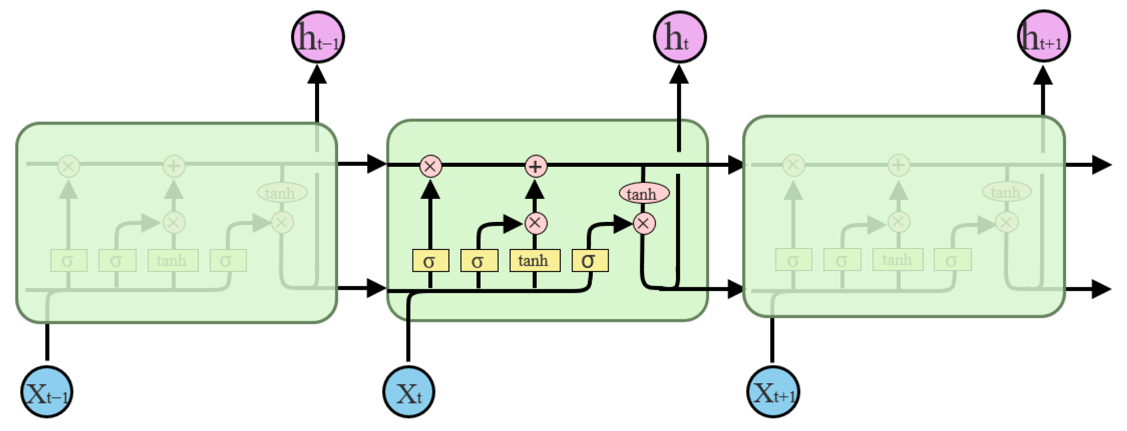
LSTM neural network belongs to the recurrent neural network (RNN), which is a special recurrent neural network improved by RNN. The basic recurrent neural network has a self-connected hidden layer structure that is not available in ordinary neural networks. It can update the hidden layer state at the current time with the hidden layer state at the previous time, which makes RNN suitable for processing time-series data. However, with the increase in time series length, RNN will become difficult to train due to “forgetting” of the early time-series information, and the gradient will disappear or explode. In contrast, LSTM solves the problem of RNN that cannot fully employ the historical information and is often used to solve the problem of long-term dependence. LSTM adds a storage cell state in the hidden layer neural node to store the past information, and uses three gates (input gate, forget gate, output gate) to control the forgetting and updating of historical information. The hidden layer is shown in Figure 2. The detailed calculation process under time step t is as follows:
(a)
Forget gate: Calculate forget gate f t by inputting data x t and outputting data h t 1 through the input gate, output a value (0~1) and transfer it to the cell state information C t 1 , and consider whether the previous cell state C t 1 is retained.
f t = σ ( W f x t + U f h t 1 + b f )
(b)
Input Gate: Update input information i t and candidate cell state C ¯ t .
i t = σ ( W i x t + U i h t 1 + b i )
C ¯ t = tanh ( W c x t + U c h t 1 + b c )
(c)
Update cell state: According to the updated candidate cell state C ¯ t and the cell state of the previous time step C t 1 , the cell state of t time step C t is updated.
C t = f t * C t 1 + i t * C ¯ t
(d)
Output gate: Use output gate o t and output cell state C t to obtain output data h t .
o t = σ ( W o x t + U o h t 1 + b o )
h t = o t * tanh ( C t )
where W f , U f and b f are the forget gate’s input weights, recurrent weights and bias, respectively, W i , U i and b i are the input gate’s input weights, recurrent weights and bias, respectively, W o , U o and b o are the output gate’s input weights, recurrent weights and bias, respectively. Activation function is expressed as
σ ( x ) = 1 1 + e x
tanh ( x ) = e x e x e x + e x

2.3. The CNN-LSTM Framework

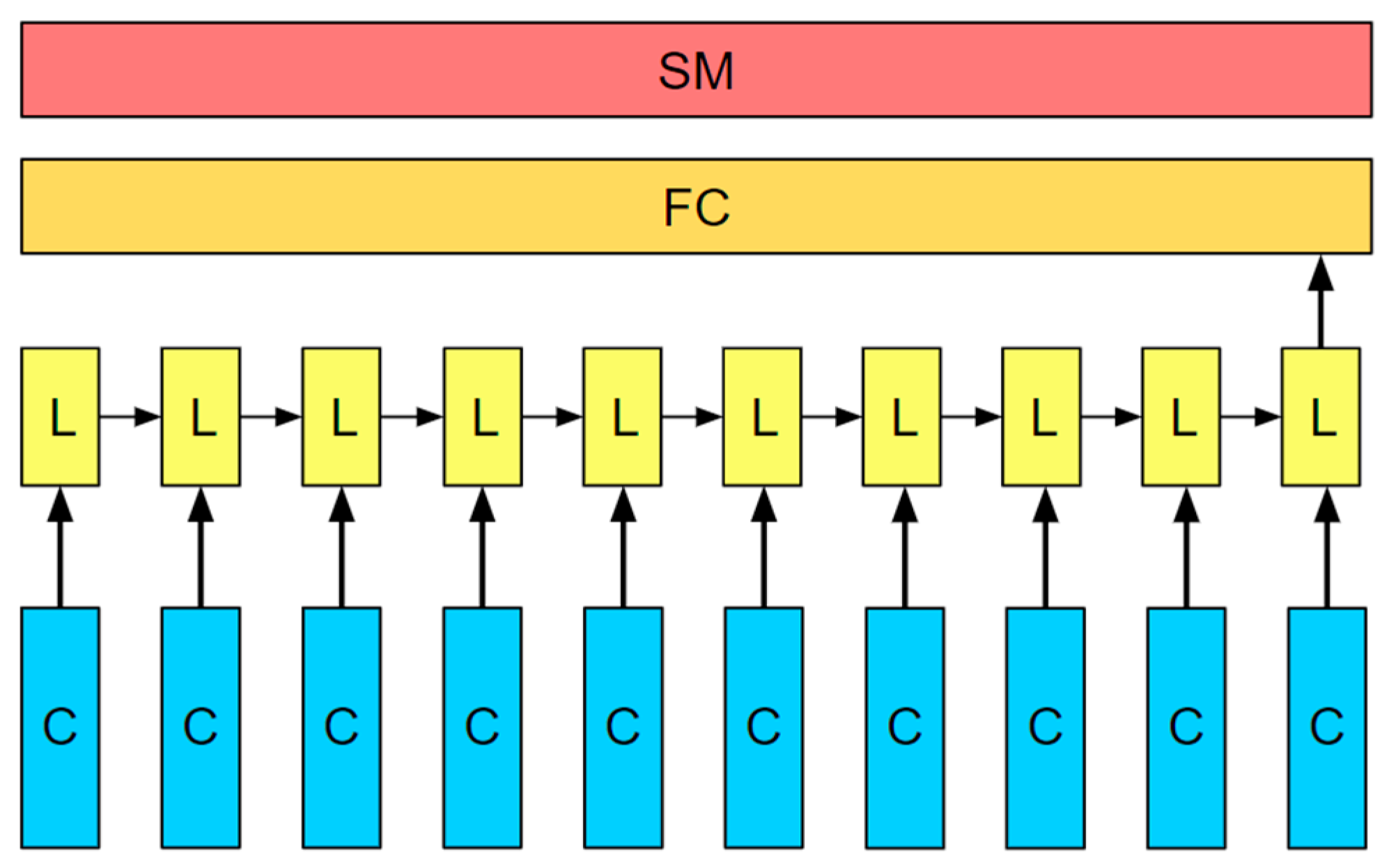
The productivity of oil wells is a function of time and multiple factors, which is a typical time series. In order to better capture and extract local features, CNN-LSTM model is used for time-series forecasting. The architecture of the proposed CNN-LSTM model is shown in Figure 3. The influencing factors of oil rate determine the dimension of input data. First, the sample features are mapped to high-dimensional space through CNN to obtain local features, and then LSTM layer is embedded to store and extract high-dimensional information. Finally, the hidden state of LSTM is mapped to productivity space using the full connection layer. In the training process, the adaptive moment estimation (ADAM) and the mean square error (MSE) are used as optimizer and loss function.
The novelty of our work is in absorbing the advantages of each neural network and making up for the limitations of a single neural network. The ability of CNN to extract deep features has been proved in the field of computer vision. The LSTM neural network is also often used for time-series and natural language processing research. Combining the two models, a hybrid model is proposed. Through the first stage of CNN deep feature extraction, the time series is endowed with high-dimensional features through the feature engineering method of neural network. The feature dimension and generalization ability are balanced through the convolution layer and pooling layer of CNN, and then the high-dimensional features processed by CNN are trained and inferred by LSTM. The LSTM memory mechanism helps the model selectively retain the memory of deep features. Because it is difficult to capture the features of extreme points in time series in training with LSTM, CNN is used to expand the features from low-dimensional space to high-dimensional space to obtain richer feature semantics. The inference ability of the proposed model is greatly improved.

2.4. Basic Theory of PSO

Generally, in the process of training the neural network model, in addition to iteratively updating the network parameters through the loss function and optimizer, there are also some parameters that need to be manually adjusted by engineers. These parameters are called hyperparameters. These hyperparameters have a significant impact on the prediction performance of the CNN-LSTM model on oil rate, such as the time window (oil rate at the previous time step) and the quantity of neurons in hidden layer. Adjusting these parameters manually is time consuming and tedious. Therefore, in order to improve the performance and training efficiency of the model, PSO is used to automatically adjust the number of LSTM neurons and the size of the time window.
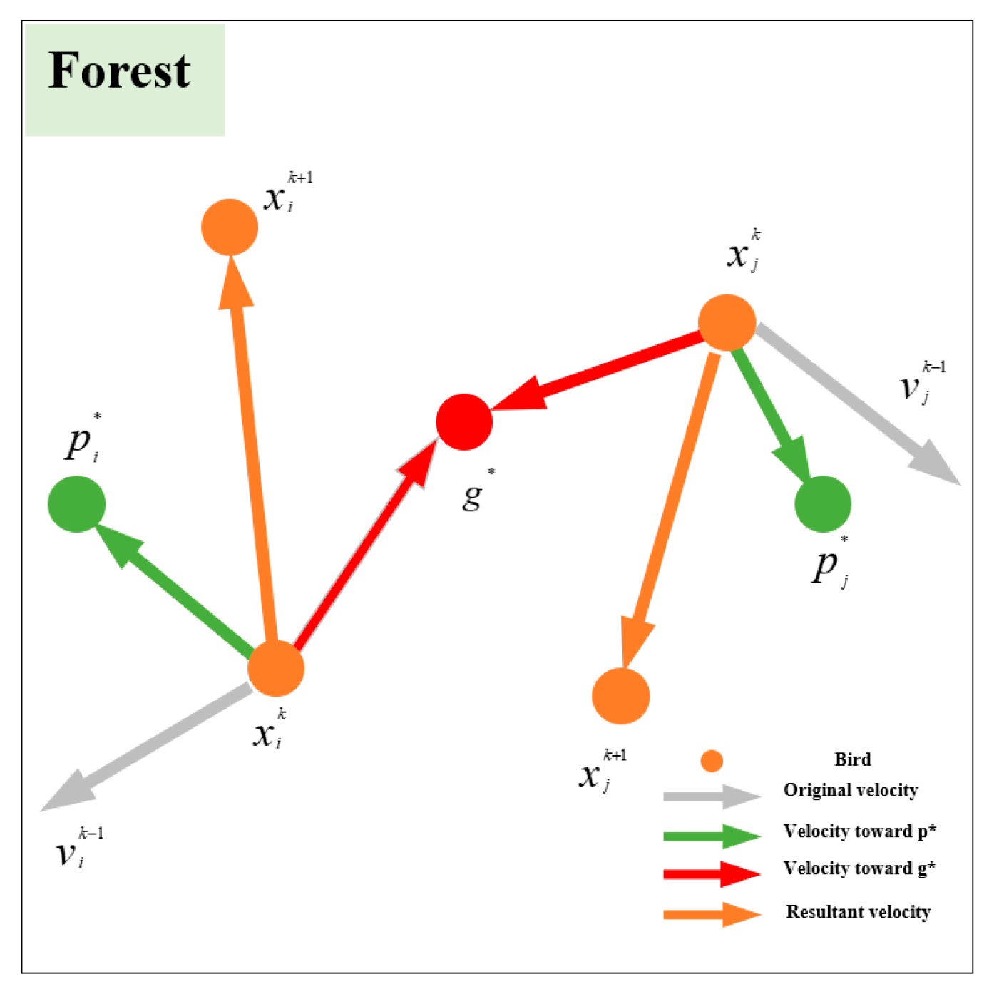
Particle Swarm Optimization, which is a kind of heuristic optimization algorithm, was proposed by Kennedy and Eberhart. It seeks the optimal solution by imitating the feeding process of birds, and has the advantages of stability, easy convergence and simple implementation [42,43]. The algorithm imitates the foraging process of birds to find the optimal solution. In the process of particle swarm optimization, the position and speed of particles themselves are updated by individual extreme value and group extreme value. The particle position is recorded as p i k , the individual extreme value is the position where the single particle has the smallest error in its own moving track, which is recorded as p i * , and the group extreme value is the position where a particle has the smallest error in its moving track, which is recorded as g*. The update speed and update position of the particles themselves are updated iteratively. Figure 4 shows that the algorithm uses p* and g* to conduct the particle swarm to adjust its flight direction, and updates the particle position until termination conditions are met. The iteration of velocity and position is shown in Equations (10) and (11).
v i k + 1 = ω v i k + c 1 r 1 ( p i * x i k ) + c 2 r 2 ( g * x i k )
x i k + 1 = x i k + v i k + 1
where v i k and x i k are the velocity and position vector for the particle i at the kth iterations, respectively. p i * is the best individual particle position, ω is the inertia weight, and g* is the global best position. c i is the member of positive acceleration constants standing for personal and global nature of the swarm. r i represents random values between 0 and 1.

2.5. Description of Mathematical Model

The proposed model is used to solve the problem of production time-series data prediction of oil reservoirs and to infer the future production status through historical data. The size of the history window and the number of neurons in the hybrid neural network are two hyperparameters that serve as the search space and model constraints of PSO. The size of the history window ranges from 1 to 10 and the number of neurons ranges from 1 to 20. Through continuous iteration, these are optimized to fix the input data and model structure. During each iteration, the model will infer future production data based on historical data. In order to evaluate the performance of the model, the following MSE is used as the objective function:
M S E = 1 n i = 1 n ( y i y ¯ i ) 2
where y i and y ¯ i are the i t h actual value and predict value, respectively. In the training process, ADAM is used as the optimization parameter of the optimizer.

2.6. Model Evaluation Criteria

Several indicators such as mean absolute error (MAE), mean absolute percentage error (MAPE), and root mean square error (RMSE) can be used to estimate the model’s performance. MAE represents the average difference between the actual data and the model results. RMSE calculates the standard deviation between the actual data and the model results. MAPE represents the forecast accuracy as a percentage. The smaller the three values, the better the performance of the model. These three criteria are defined as follows:
M A P E = ( 1 n i = 1 y i y ¯ i y i ) × 100
M A E = 1 n i = 1 n y i y ¯ i
R M S E = 1 n i = 1 n ( y i y ¯ i ) 2
where y i and y ¯ i are the i t h actual value and predict value, respectively.
The indicators mentioned above are commonly used evaluation indicators for time-series forecast, and comprehensive consideration of multiple measures can further analyze the model. For a single indicator, if the absolute error between the real value and the predicted value is valued, MAE is selected, and MAE is sensitive to extreme values. If the square of the difference between the real value and the predicted value is valued, RMSE is selected. If there is a magnitude difference between the real values of different samples or more attention is paid to the percentage difference between the predicted value and the real value, MAPE is preferred. For the cooperation of multiple indicators, MAE and RMSE can be used together to see the dispersion of sample error. MAE and MAPE can be used together to estimate the fitting degree of the model to samples of different orders of magnitude. Therefore, we can better evaluate the model performance by using the combination of these three evaluation indicators.

3. Results and Discussion

3.1. The Complete Workflow of the Case Study

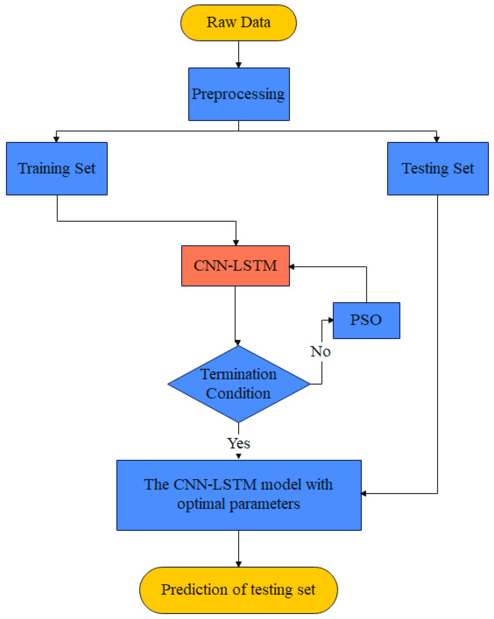
According to the experimental results of volcanic rock reservoirs in Xinjiang, it is impossible to maintain formation pressure or improve oil recovery through water drive due to the development of natural fractures in volcanic rock reservoirs. Most volcanic reservoirs are developed by depletion-drive development, and liquid rate is influenced by the choke size. Therefore, the input data includes the historical liquid rate in the time window and the choke size at the predicted time. The label is the oil rate at the prediction time. The overall process is shown in Figure 5. The steps in the whole process are as follows:
Step 1. Preprocess the original data. First, the original data are denoised to remove the outliers. The dataset is then normalized according to Equation (16) in order to avoid disturbing the results of the CNN-LSTM model with large or small values.
x n e w = x o l d x min x max x min
where x n e w is the normalized value, while x o l d , x min and x max are the real values and the minimum and maximum of the sample.
After preprocessing, according to the above feature description and the CNN-LSTM network structure, the model is described as follows:
Y ( t ) = F ( X ( t ) , Y ( t 1 ) , Y ( t 2 ) , , Y ( t 3 ) )
where Y ( t ) is the predicted oil rate at the time step t. F ( ) represents proposed model operation. X ( t ) is the choke size at the time step t.
Step 2. Conduct model training. The data set is divided into two parts, and the ratio of general training set and test set is 4:1. Use training sets when training models. The number of neurons in the model and the size of the time window are optimized by PSO according to Figure 5 during the training stage. The input and output forms are as follows:
{ X ( 4 ) Y ( 1 ) Y ( 2 ) Y ( 3 ) X ( 5 ) Y ( 2 ) Y ( 3 ) Y ( 4 ) X ( t ) Y ( t 3 ) Y ( t 2 ) Y ( t 1 ) i n p u t Y ( 4 ) Y ( 5 ) Y ( t ) } o u t p u t
Step 3. Conduct model predicting. Because there is future information in the test set, it may interfere with the model prediction results. In order to evaluate the prediction performance of the model accurately, the test set cannot be directly input into the model for prediction*. Instead, the test set needs to be updated iteratively with the predicted values predicted by the model. After the update, the input model can continue to be iterated. The input and output forms are as follows:
{ X ( t + 1 ) Y ( t 2 ) Y ( t 1 ) Y ( t ) X ( t + 2 ) Y ( t 1 ) Y ( t ) Y ( t + 1 ) X ( t + n ) Y ( t + n 3 ) Y ( t + n 2 ) Y ( t + n 1 ) i n p u t Y ( t + 1 ) Y ( t + 2 ) Y ( t + n ) } o u t p u t
where Y ( t + n ) represents oil rate at the time step t + n . It is worth noting that the results obtained from the test set are normalized, and the future productivity is obtained after the results are de-normalized. The proposed neural network model is built using pytorch [44], which is a deep learning framework. The workflow shown in Figure 5 is implemented using Python 3.8.

3.2. Complex Production Variation

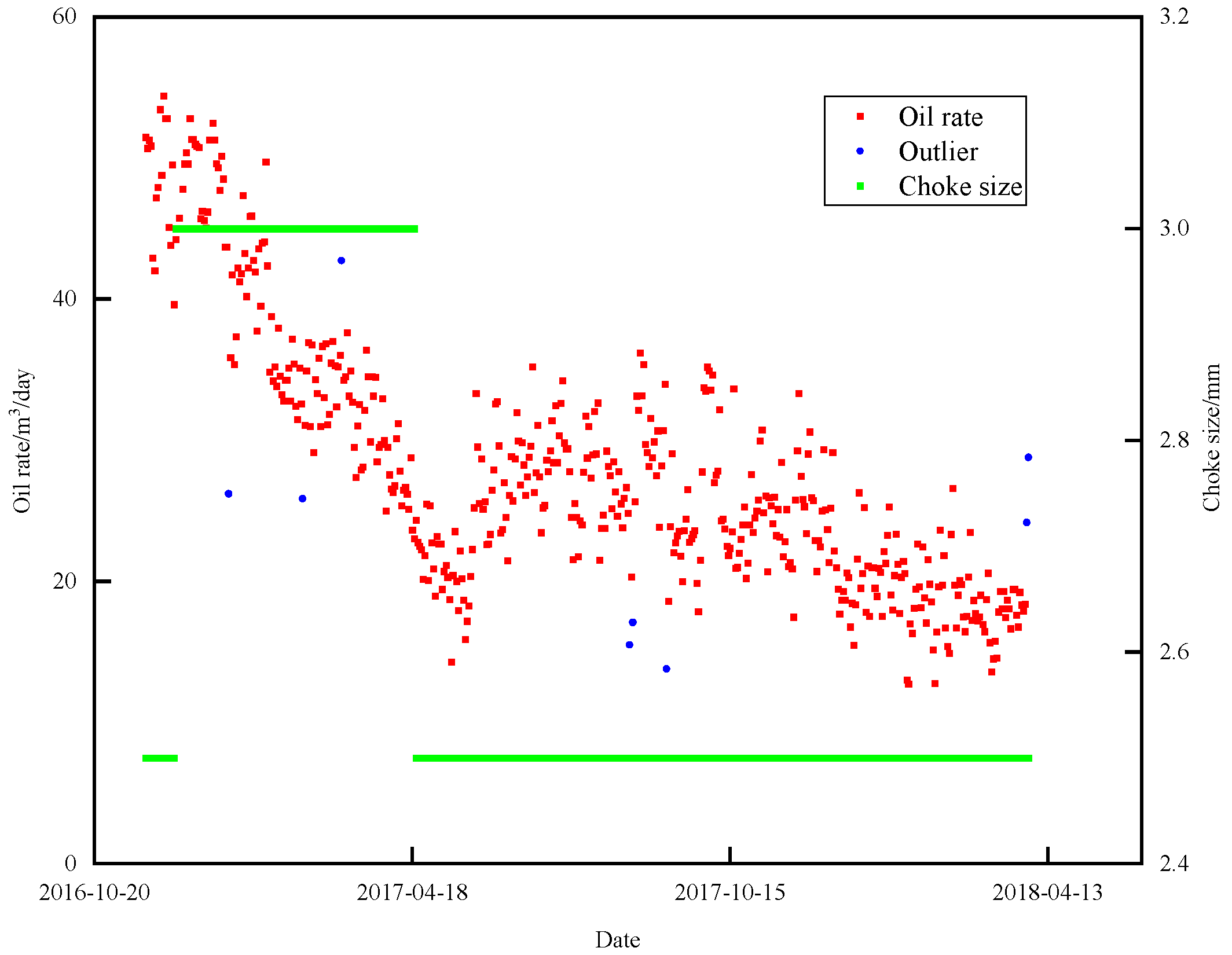
In the process of oilfield development, the operations of shut-ins and choke size adjustment occur frequently. The actual oil rate is not continuous and smooth, but rather discontinuous. Therefore, traditional methods are difficult to predict accurately. In this section, data are collected from a fractured horizontal well in Xinjiang volcanic reservoirs in northwest China. The data set includes oil rate and choke size of 17 months, with a total of 501 data points, as shown in Figure 6. The initial choke size is 2.5~3 mm. Due to the decrease in oil rate, it will be adjusted from 3 mm to 2.5 mm later. Local Outlier Factor method [45] is used to detect outliers in the data set, that is, the blue circle data in Figure 6, and the outliers are replaced by the average values of the oil rate at the front and back times. After denoising, the data are normalized, and the normalized data are input into the CNN-LSTM model. The autoregressive moving average model (ARMA) and the autoregressive integrated moving average model (ARIMA) cannot be used in this complex case because the input items contain multiple values such as oil rate and choke size. In order to better evaluate the performance of the proposed model, fully connected ANN, traditional descent curve, RNN and LSTM models are used to compare with CNN-LSTM models.
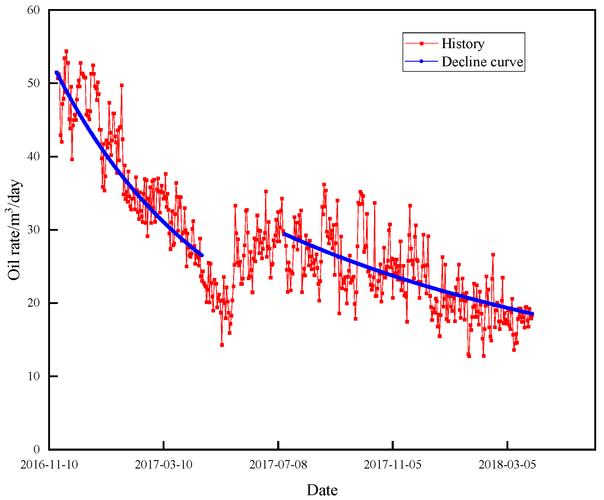
As shown in Figure 7, the decline curve analysis is used to predict the oil rate. According to the actual production data, the harmonic decline method is used to divide the entire historical cycle into two parts according to the production constraint data such as the choke size. The decline index and initial decline rate obtained from the previous analysis are 0.4 and 0.005, respectively. The later values of the other part are 0.5 and 0.002, respectively.
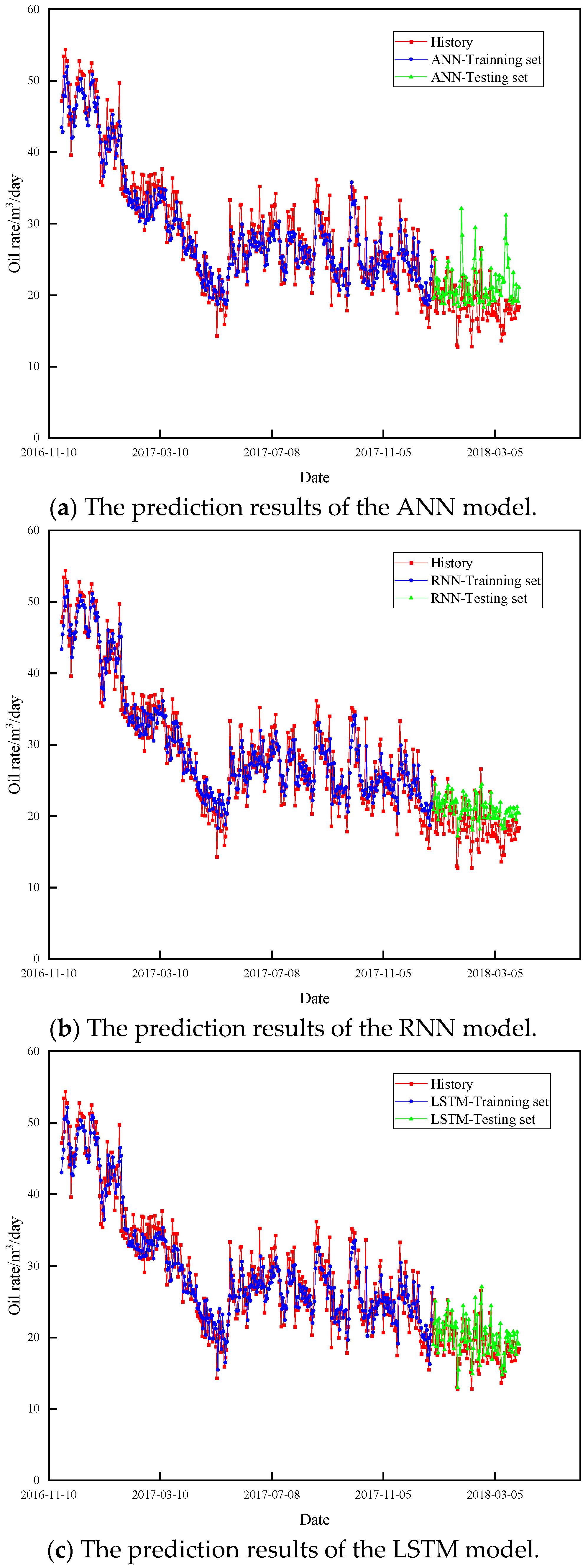
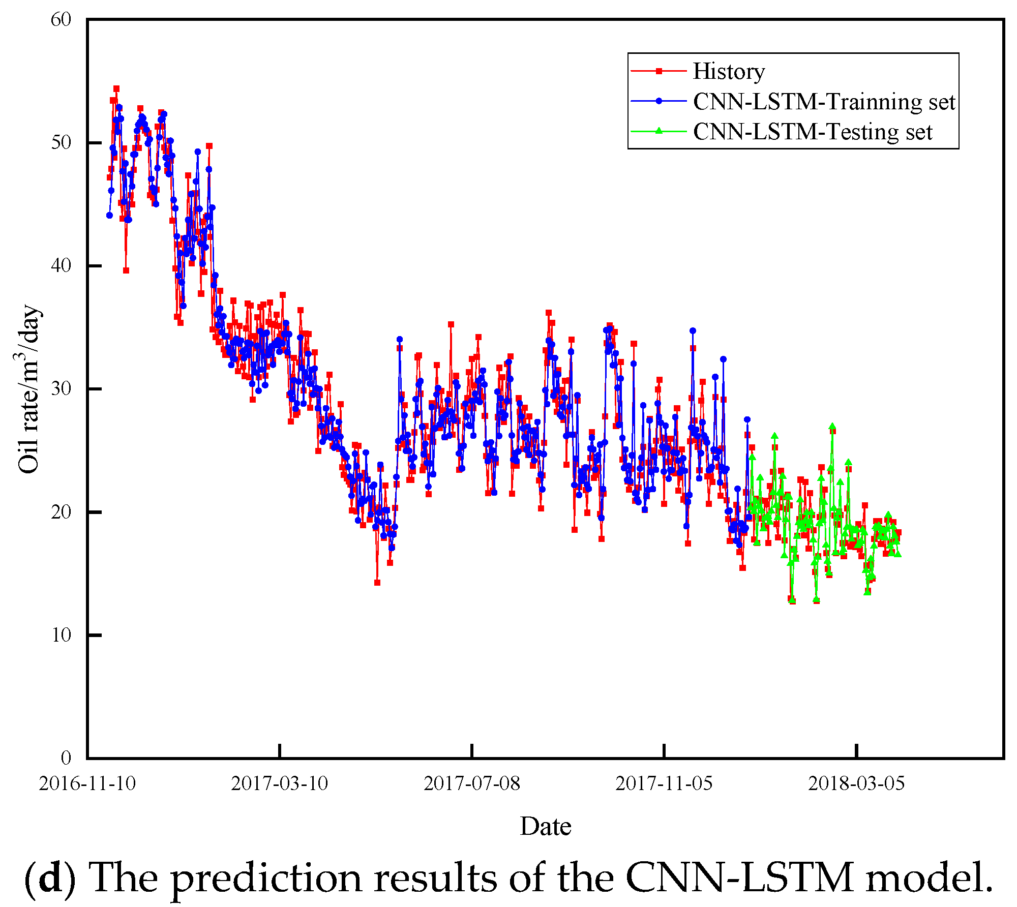
The CNN-LSTM model is trained according to the process shown in Figure 5. The hyperparameters including time window size and the quantity of neurons obtained by PSO are 6 and 15, respectively. According to the optimization result, the LSTM, ANN, RNN and other models for comparison use the same hyperparameters. The training and prediction results of the four models are shown in Figure 8. For ANN and RNN, the details of training results are better than those of the prediction results, and the fitting effect of most data in the prediction stage is poor, indicating that the model generalization ability is poor. For LSTM, the overall fitting effect is better than that of RNN and ANN, but the fitting effect of some data in the prediction stage is poor. For CNN-LSTM, the prediction results fit well and the generalization ability is better than that of ANN, RNN and LSTM.
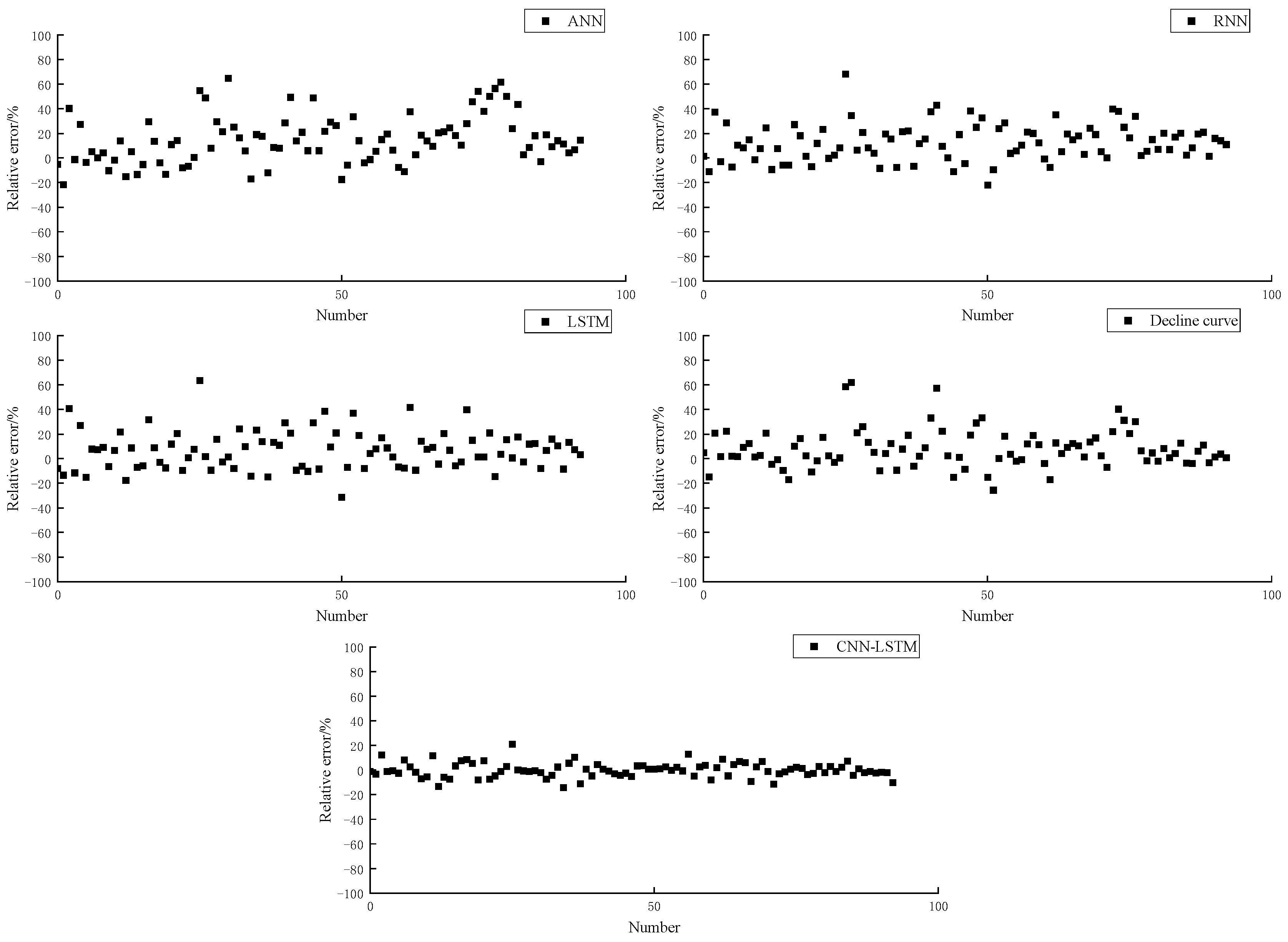
The relative error analysis between the testing results of ANN, decline curve analysis, RNN, LSTM and CNN-LSTM models and the real values is shown in Figure 9. For the results of ANN and RNN, multiple error values are distributed beyond 20%, some errors will be close to 60–80%. For LSTM and decline curve, although the error is obviously smaller than that of traditional neural network, there are still some error points close to 60%. As for CNN-LSTM, most errors are within 20%, and individual error points fall within 20–40%. Through comparison, it can be concluded that the proposed model can accurately predict the global trend and local single value of oil production time series.
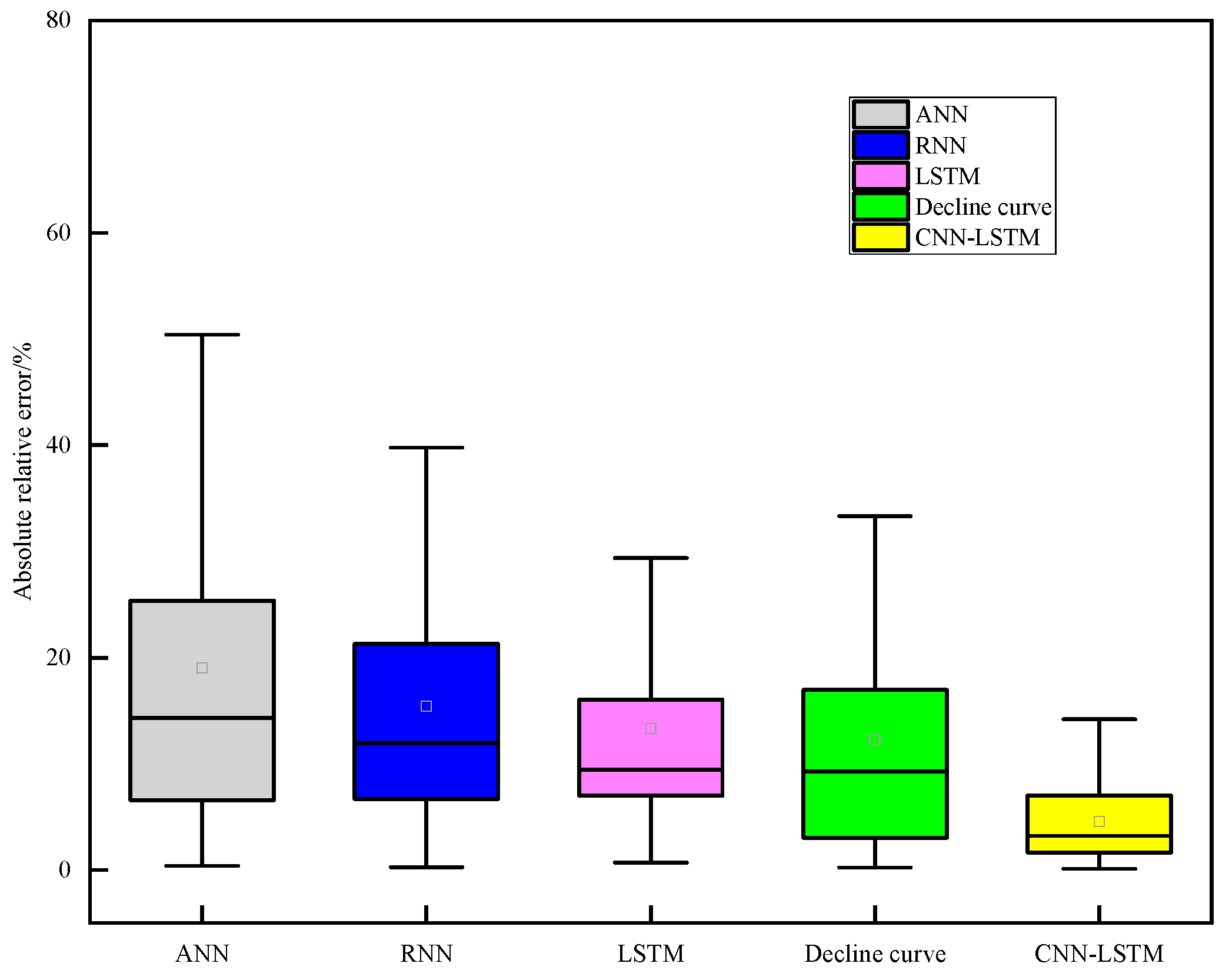
The absolute values of the relative errors of the five models are analyzed using the box chart. The results are shown in Figure 10. For the ANN and RNN models, the relative errors of about 25% error points are greater than 20%, indicating that the two models have poor effects on oil production prediction. It is not recommended to directly use these two models for prediction. For the decline curve, the results show that the prediction results are better than those of the first two models. For LSTM, the absolute value of about 75% error is within 20%, and the value of 50% is less than 10%. For the CNN-LSTM model, 75% of the data is less than 10%, which is better than the other four methods.
MAPE, MAE and RMSE are calculated based on the predicted results and real values of the five models. The calculation results are shown in Table 2. The statistical evaluation indicators of ANN and RNN are significantly lower than those of the other three models. For CNN-LSTM, the statistical indicators of model results are 5.5% (MAPE), 1.15 (MAE) and 1.54 (RMSE), respectively. The smaller statistical indicators show that the generalization ability of the proposed model is better than that of other models. The results show that the proposed model can accurately predict the global trend and local single value of oil production time series.

3.3. Comparison and Discussion with Decline Curve Analysis

For a long time in the past, reservoir engineers usually used decline curve analysis to study the production of oil wells for the prediction of production changes. Therefore, the proposed model and decline curve analysis are compared and discussed.
The decline curve analysis method is a flexible and simple reservoir engineering method. The engineers can analyze the decline curve of historical data through charts or fitting calculation so as to predict the future production change. Generally, the production decline pattern of an oilfield is relatively fixed, and the decline curve and trend are basically similar. For the model proposed in this paper, different training data sets have different models. It can be seen from Figure 7 and Figure 8 that the decline curve analysis focuses on the overall trend change while ignoring the instantaneous fluctuation of production due to engineering and geological factors, which leads to the decline of prediction accuracy. The proposed model can not only capture the trend of global output change, but also capture the change in extreme value, greatly improving the accuracy of prediction.

4. Conclusions

In this study, a hybrid forecasting model (CNN-LSTM) based on a convolutional neural network (CNN) and a Long Short-Term Memory (LSTM) neural network is proposed and used to predict the production of fractured horizontal wells in volcanic reservoirs. The model solves the limitation of traditional methods that rely on personal experience. The certain hyperparameters of the whole model are optimized by PSO. In order to evaluate the model, some production dynamics from the Xinjiang oilfield of China are used for comparative analysis. The experimental results show that the CNN-LSTM model is superior to traditional neural networks and conventional decline curves. The main conclusions are as follows:
(1) The CNN network and LSTM network in machine learning are applied to the production dynamic analysis, and the PSO is used to optimize the neural network to achieve accurate prediction of oil well production performance.
(2) PSO is used to optimize the proposed neural network model, realizing the automatic optimization of neural network hyperparameters, avoiding the tedious parameter adjustment process of conventional neural network, greatly simplifying the optimization process of prediction model, simple operation, and convenient for automation and on-site personnel.
(3) The case study shows that the established production dynamic prediction model can accurately predict the future production dynamic changes, the average absolute percentage error is less than 10%, and the prediction accuracy meets the on-site requirements.
The proposed model can be applied to the prediction of oil and gas reservoir performance data. It not only supports multivariate and univariate time series prediction, but also supports flexible change in window size. However, the limitation of the model is that it can only predict the production time series data of a single well, and cannot consider the interference of multi-well multi-time series. Thus, we intend to study the interconnection of neural networks and attention mechanism to deal with time–space correlation production prediction of different wells in the future.

Author Contributions

Conceptualization, J.W. and Z.R.; methodology, J.W.; software, J.W.; validation, J.W. and H.W.; formal analysis, J.W.; investigation, Z.R.; resources, Y.W.; data curation, X.Q.; writing—original draft preparation, J.W.; writing—review and editing, S.W.; visualization, J.W. and H.W.; supervision, S.W.; project administration, Y.W.; funding acquisition, J.W. All authors have read and agreed to the published version of the manuscript.

Funding

This research received no external funding.

Institutional Review Board Statement

Not applicable.

Data Availability Statement

The data presented in this study are available on request from the corresponding author. The data are not publicly available because it is confidential.

Conflicts of Interest

The authors declare no conflict of interest.

References

  1. Amirian, E.; Dejam, M.; Chen, Z. Performance forecasting for polymer flooding in heavy oil reservoirs. Fuel 2018, 216, 83–100. [Google Scholar] [CrossRef]
  2. Nwaobi, U.; Anandarajah, G. Parameter determination for a numerical approach to undeveloped shale gas production estimation: The UK Bowland shale region application. J. Nat. Gas Sci. Eng. 2018, 58, 80–91. [Google Scholar] [CrossRef]
  3. Clarkson, C.R.; Williams-Kovacs, J.D. History-matching and forecasting tight/shale gas condensate wells using combined analytical, semi-analytical, and empirical methods. J. Nat. Gas Sci. Eng. 2015, 26, 1620–1647. [Google Scholar] [CrossRef]
  4. Kalra, S.; Tian, W. A numerical simulation study of CO 2 injection for enhancing hydrocarbon recovery and sequestration in liquid-rich shales. Pet. Sci. 2018, 15, 103–115. [Google Scholar] [CrossRef] [Green Version]
  5. Zhang, R.H.; Zhang, L.H.; Tang, H.Y. A simulator for production prediction of multistage fractured horizontal well in shale gas reservoir considering complex fracture geometry. J. Nat. Gas Sci. Eng. 2019, 67, 14–29. [Google Scholar] [CrossRef]
  6. Clarkson, C.R.; Qanbari, F. A semi-analytical method for forecasting wells completed in low permeability, undersaturated CBM reservoirs. J. Nat. Gas Sci. Eng. 2016, 30, 19–27. [Google Scholar] [CrossRef]
  7. Du, D.F.; Wang, Y.Y.; Zhao, Y.W. A new mathematical model for horizontal wells with variable density perforation completion in bottom water reservoirs. Pet. Sci. 2017, 14, 383–394. [Google Scholar] [CrossRef] [Green Version]
  8. Schuetter, J.; Mishra, S.; Zhong, M.; LaFollette, R. A data-analytics tutorial: Building predictive models for oil production in an unconventional shale reservoir. SPE J. 2018, 23, 1–75. [Google Scholar] [CrossRef]
  9. Luo, G.; Tian, Y.; Bychina, M.; Ehlig-Economides, C. Production optimization using machine learning in Bakken shale. In Proceedings of the Unconventional Resources Technology Conference, Houston, TX, USA, 23–25 July 2018. [Google Scholar]
  10. Wang, S.; Chen, S. Insights to fracture stimulation design in unconventional reservoirs based on machine learning modeling. J. Pet. Sci. Eng. 2019, 174, 682–695. [Google Scholar] [CrossRef]
  11. Panja, P.; Velasco, R.; Pathak, M.; Deo, M. Application of artificial intelligence to forecast hydrocarbon production from shales. Petroleum 2018, 4, 75–89. [Google Scholar] [CrossRef]
  12. Han, B.; Bian, X. A hybrid PSO-SVM-based model for determination of oil recovery factor in the low-permeability reservoir. Petroleum 2018, 4, 43–49. [Google Scholar] [CrossRef]
  13. Zhong, M.; Schuetter, J.; Mishra, S. Do data mining methods matter? A Wolfcamp Shale case study. In Proceedings of the SPE Hydraulic Fracturing Technology Conference, Woodlands, TX, USA, 23–25 January 2018. [Google Scholar]
  14. Cao, Q.; Banerjee, R.; Gupta, S.; Li, J.; Zhou, W.; Jeyachandra, B. Data driven production forecasting using machine learning. In Proceedings of the SPE Argentina Exploration and Production of Unconventional Resources Symposium, Buenos Aires, Argentina, 1–3 June 2016. [Google Scholar]
  15. Ahmadi, M.A.; Ebadi, M.; Shokrollahi, A.; Majidi, S.M.J. Evolving artificial neural network and imperialist competitive algorithm for prediction oil flow rate of the reservoir. Appl. Soft Comput. 2013, 13, 1085–1098. [Google Scholar] [CrossRef]
  16. Fulford, D.S.; Bowie, B. Machine learning as a reliable technology for evaluating time-rate performance of unconventional wells. SPE Econ. Manag. 2015, 8, 23–39. [Google Scholar] [CrossRef]
  17. Li, D.; Wang, Z.; Zha, W.; Wang, J.; He, Y.; Huang, X.; Du, Y. Predicting production-rate using wellhead pressure for shale gas well based on Temporal Convolutional Network. J. Petrol. Sci. Eng. 2022, 216, 110644. [Google Scholar] [CrossRef]
  18. Wang, H.; Mu, L.; Shi, F.; Dou, H. Production prediction at ultra-high water cut stage via recurrent neural network. Petrol. Explor. Dev. 2020, 47, 1084–1090. [Google Scholar] [CrossRef]
  19. Cheng, Y.; Yang, Y. Prediction of oil well production based on the time series model of optimized recursive neural network. Petrol. Sci. Technol. 2021, 39, 303–312. [Google Scholar] [CrossRef]
  20. Al-Shabandar, R.; Jaddoa, A.; Liatsis, P.; Hussain, A.J. A deep gated recurrent neural network for petroleum production forecasting. Mach. Learn. Appl. 2020, 3, 100013. [Google Scholar] [CrossRef]
  21. Mahzari, P.; Emambakhsh, M.; Temizel, C.; PJones, A. Oil production forecasting using deep learning for shale oil wells under variable gas-oil and water-oil ratios. Petrol. Sci. Technol. 2022, 40, 445–468. [Google Scholar] [CrossRef]
  22. Zha, W.; Liu, Y.; Wan, Y.; Luo, R.; Li, D.; Yang, S.; Xu, Y. Forecasting monthly gas field production based on the CNN-LSTM model. Energy 2022, 260, 124889. [Google Scholar] [CrossRef]
  23. Zhang, J.; Zhu, Y.; Zhang, X.; Ye, M. Developing a Long Short-Term Memory (LSTM) based model for predicting water table depth in agricultural areas. J. Hydrol. 2018, 561, 918–929. [Google Scholar] [CrossRef]
  24. Zhang, D.; Chen, Y.; Meng, J. Synthetic well logs generation via recurrent neural networks. Pet. Explor. Dev. 2018, 45, 598–607. [Google Scholar] [CrossRef]
  25. Qin, Y.; Li, K.; Liang, Z.; Lee, B.; Zhang, F. Hybrid forecasting model based on long short term memory network and deep learning neural network for wind signal. Appl. Energy 2019, 236, 262–272. [Google Scholar] [CrossRef]
  26. Han, S.; Qiao, Y.H.; Yan, J. Mid-to-long term wind and photovoltaic power generation prediction based on copula function and long short term memory network. Appl. Energy 2019, 239, 181–191. [Google Scholar] [CrossRef]
  27. Li, Y.; Cao, H. Prediction for tourism flow based on LSTM Neural Network. Procedia Comput. Sci. 2018, 129, 277–283. [Google Scholar] [CrossRef]
  28. Tong, W.; Li, L.; Zhou, X.; Hamilton, A.; Zhang, K. Deep learning PM2.5 concentrations with bidirectional LSTM RNN. Air Qual. Atmos. Health 2019, 12, 411–423. [Google Scholar] [CrossRef]
  29. Xuanyi, S.; Yuetian, L.; Liang, X. Time-series well performance prediction based on Long Short-Term Memory (LSTM) neural network model. J. Pet. Sci. Eng. 2020, 186, 1–14. [Google Scholar]
  30. Xue, L.; Gu, S.; Wang, J.; Liu, Y. Production dynamic prediction of gas well based on particle swarm optimization and long short-term memory. Oil Drill. Prod. Technol. 2021, 45, 525–531. [Google Scholar]
  31. Zheng, J.; Du, J.; Liang, Y. Research into real-time monitoring of shutdown pressures in multi-product pipelines. Pet. Sci. Bull. 2021, 4, 648–656. [Google Scholar]
  32. Luo, G.; Xiao, L.; Shi, Y.; Shao, R. Machine learning for reservoir fluid identification with logs. Pet. Sci. Bull. 2022, 1, 24–33. [Google Scholar]
  33. Hu, X.; Tu, Z.; Luo, Y.; Zhou, F.; Li, Y.; Liu, J.; Yi, P. Shale gas well productivity prediction model with fitted function-neural network cooperation. Pet. Sci. Bull. 2022, 03, 394–405. [Google Scholar]
  34. Song, X.; Yao, X.; Li, G.; Xiao, L.; Zhu, Z. A novel method to calculate formation pressure based on the LSTM-BP neural network. Pet. Sci. Bull. 2022, 1, 12–23. [Google Scholar]
  35. Spandonidis, C.; Theodoropoulos, P.; Giannopoulos, F.; Galiatsatos, N.; Petsa, A. Evaluation of deep learning approaches for oil & gas pipeline leak detection using wireless sensor networks. Eng. Appl. Artif. Intell. 2022, 113, 104890. [Google Scholar]
  36. Spandonidis, C.; Theodoropoulos, P.; Giannopoulos, F. A Combined Semi-Supervised Deep Learning Method for Oil Leak Detection in Pipelines Using IIoT at the Edge. Sensors 2022, 22, 4105. [Google Scholar] [CrossRef] [PubMed]
  37. Li, Q.; Shi, Y.; Lin, R.; Qiao, W.; Ba, W. A novel oil pipeline leakage detection method based on the sparrow search algorithm and CNN. Measurement 2022, 204, 112122. [Google Scholar] [CrossRef]
  38. Xueqing, Z.; Fang, L. Real time prediction of China’s carbon emissions based on CNN-LSTM model. China Arab. Sci. Technol. Forum 2022, 2022, 5. [Google Scholar]
  39. Ke, Z.; Renchuan, Z. A CNN-LSTM Ship Motition Extrem Value Prediction Mode. J. Shanghai Jiaotong Univ. 2022, 89, 5. [Google Scholar]
  40. LeCun, Y. Generalization and network design strategies. In Technical Report CRG-TR-89-4; University of Toronto: Toronto, ON, Canada, 4 June 1989. [Google Scholar]
  41. Zhao, J.; Bai, G.; Li, Y. Short-term wind power predicttion based on CNN-LSTM. Pro. Auto. Instru. 2020, 41, 37–41. [Google Scholar]
  42. Niknam, T. A new fuzzy adaptive hybrid particle swarm optimization algorithm for non-linear, non-smooth and non-convex economic dispatch problem. Appl. Energy 2010, 87, 327–339. [Google Scholar] [CrossRef]
  43. Kennedy, J.; Eberhart, R. Particle swarm optimization. In Proceedings of the IEEE International Conference on Neural Networks, Perth, Australia, 27–30 November 1995. [Google Scholar]
  44. Pytorch Documentation. Available online: https://pytorch.org (accessed on 1 June 2022).
  45. Breunig, M.M.; Kriegel, H.P.; Ng, R.T.; Sander, J. LOF: Identifying density-based local outliers. In Proceedings of the SIGMOD/PODS00: ACM International Conference on Management of Data and Symposium on Principles of Database Systems, Dallas, TX, USA, 15–18 May 2000. [Google Scholar]
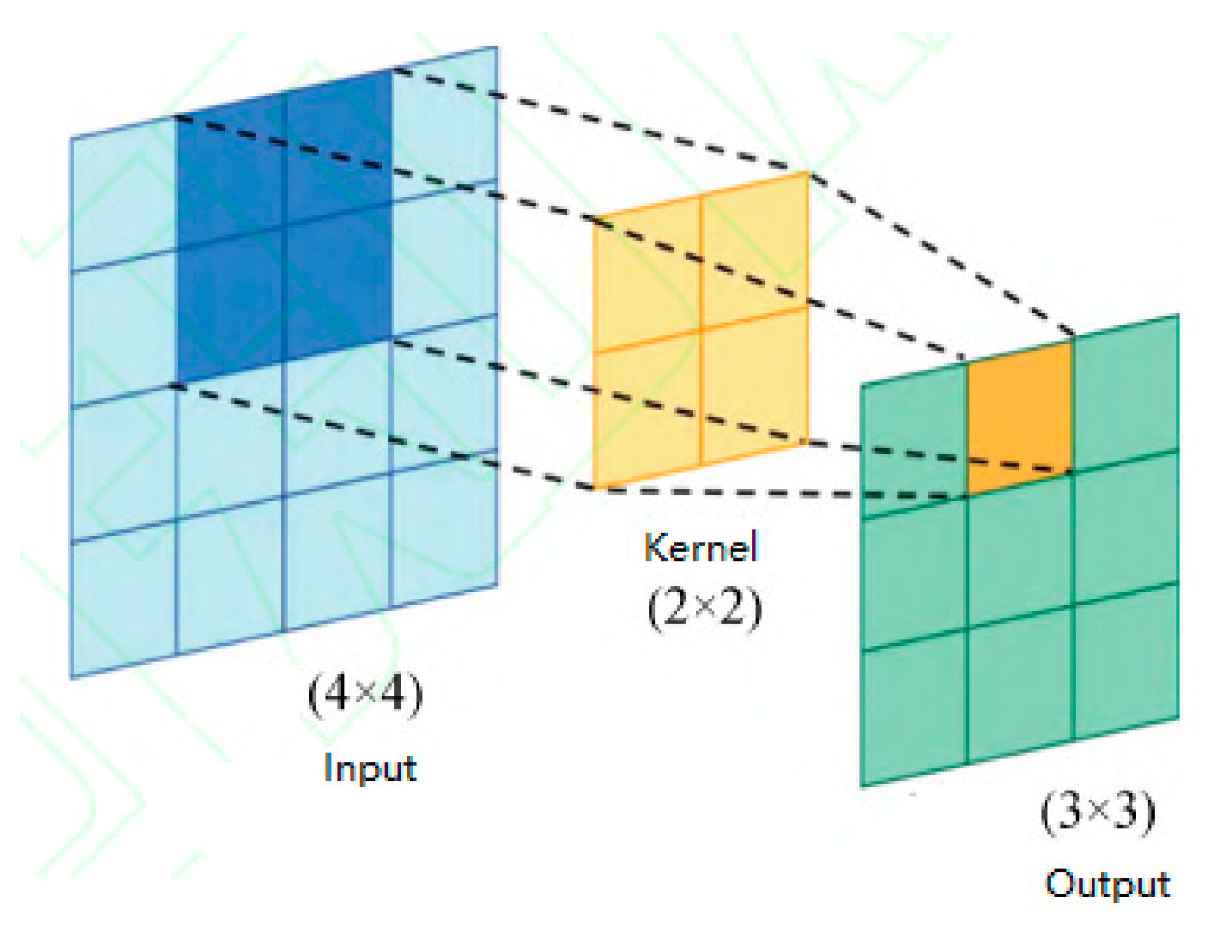
Figure 1. Convolution kernel calculation process.
Energies 16 00499 g001
Figure 2. The structure of LSTM.
Energies 16 00499 g002
Figure 3. The structure of CNN-LSTM.
Energies 16 00499 g003
Figure 4. The schematic of the optimization process of PSO.
Energies 16 00499 g004
Figure 5. Overall workflow of our suggested model.
Energies 16 00499 g005
Figure 6. The scatter diagram of on-site sample data.
Energies 16 00499 g006
Figure 7. The decline curve analysis.
Energies 16 00499 g007
Figure 8. Fitting effect of four models’ prediction results.
Energies 16 00499 g008aEnergies 16 00499 g008b
Figure 9. The relative error distribution of the five methods.
Energies 16 00499 g009
Figure 10. Absolute relative error boxplot of five models.
Energies 16 00499 g010
Table 1. The description of the symbols.
SymbolDescription
u i j k the kernel between the ith feature map of the k−1th layer and the jth feature map of the kth layer
x i k 1 the ith feature map’s output value from the k−1th layer
b j k the jth feature map’s bias from the kth layer
y j k the jth feature map’s output value from kth layer
* convolution
C j the collection of input feature maps
f ( ) activation function, which is usually sigmoid function or rectified linear unit (ReLU)
Table 2. Performance comparison for the five models.
ModelMAPEMAERMSE
ANN18.693.334.23
RNN15.412.713.26
Decline curve analysis14.152.312.73
LSTM13.532.182.48
CNN-LSTM5.491.151.54
Disclaimer/Publisher’s Note: The statements, opinions and data contained in all publications are solely those of the individual author(s) and contributor(s) and not of MDPI and/or the editor(s). MDPI and/or the editor(s) disclaim responsibility for any injury to people or property resulting from any ideas, methods, instructions or products referred to in the content.