Abstract
Accurately evaluating the fault type and location is important for ensuring the reliability of the power distribution network. A mushrooming number of distributed generations (DGs) connected to the distribution system brings challenges to traditional fault classification and location methods. Novel AI-based methods are mostly based on wide area measurement with the assistance of intelligent devices, whose economic cost is somewhat high. This paper develops a super-resolution (SR) and graph neural network (GNN) based method for fault classification and location in the power distribution network. It can accurately evaluate the fault type and location only by obtaining the measurements of some key buses in the distribution network, which reduces the construction cost of the distribution system. The IEEE 37 Bus system is used for testing the proposed method and verifying its effectiveness. In addition, further experiments show that the proposed method has a certain anti-noise capability and is robust to fault resistance change, distribution network reconfiguration, and distributed power access.
1. Introduction
The reliability of the power distribution network is crucial for ensuring the safety and stability of electricity delivered to customers [1]. To enhance the reliability of distribution networks, power system operators must deal with faults in good time. Thus, accurately locating and quickly clearing faults after the occurrence is of great concern [2]. In addition, to enable operators to properly clear the faults, accurately classifying the type of faults is also important.
There have been many pieces of research on fault classification. Threshold values and logical relationships are the main means of traditional fault-type identification. For example, [3] proposed an overcurrent protection-based fault classification method, which achieved a great identification effect at that time. However, pre-calibration for threshold is required in most of these methods, which accounts for 30% of the total cost of the workforce on setting relay thresholds [4]. Recently, artificial intelligence (AI) technology has been widely used in this field. The main methods include neural network [5], fuzzy neural network [6], Petri net [7], and so on. The fuzzy neural network, especially, has been widely adopted because of its great generalization ability and performance. In [8], a combined fuzzy-logic wavelet-based fault classification method was proposed, which achieved better performance and faster speed compared to other methods at that time. The application of AI methods has brought new developments and breakthroughs to fault-type classification.
Existing fault location methods can be divided into several categories. Impedance-based methods use voltage and current measurements to estimate fault impedance and location. Specifically, [9] developed an impedance-based fault-locating algorithm with current data as the only input, and demonstrated its efficacy with simulated and actual field data. Voltage drop-based methods analyze the voltage measurements at different buses to identify the fault location when a fault occurs. For example, in [10], a method based on matching calculated voltage sag data was proposed, which can pinpoint fault location precisely. Travelling wave-based methods adopt the reflection of high-frequency wave and time of propagation to evaluate the position of the fault [11]. Studies such as [12] used the traveling wave generated by the circuit breaker reclosing to locate faults for feeders in the power distribution network. These methods require high-time synchronization between communication devices. Recently, AI methods have been leveraged in distribution system fault locations extensively. In [13], 1-D convolutional neural network and waveform concatenation were adopted to locate the faults in resonant grounding distribution systems. The authors of [2] proposed a fault location strategy based on graph convolutional networks and measurement of buses in the distribution system, which achieved good robustness and performance.
Whether applied in fault classification or fault location, most AI methods need to utilize wide area measurements gathered from intelligent devices to locate the fault. Even if these methods crippled the influence of load change and avoided the injection of high-frequency signals, high reliance on the number of intelligent measuring devices seriously increases the construction cost. Insufficient investment would certainly increase the difficulty and time of troubleshooting. Several researchers have recently offered successful examples of how they have solved this problem. In [14], fault estimations were achieved by relating the voltage deviation measured on a small number of buses to the fault current calculated based on the bus impedance matrix, considering the fault in different points. Aiming at asymmetrical faults in distribution networks, [15] proposes a sparse measurement-based fault section location method, which can narrow the location to two adjacent nodes by few intelligent electronic devices (IEDs).
This paper proposes an SR-GNN method to solve the above problem for fault diagnosis for medium/high-voltage distribution networks. Measurements on a few critical buses are gathered by μPMU (Micro-PMU) [16] in the distribution system, which are used to reconstruct the measurements of the whole distribution network buses through the SR technology based on a graph convolutional network (GCN) [17]. The reconstructed measurements are utilized to evaluate the fault classification and location based on the graph attention network (GAT) [18]. The proposed method is tested in the IEEE 37 bus distribution system built in OpenDSS software [19]. Experimental results show that the proposed method has good adaptation and robustness to noise and fault resistance. Furthermore, the influence of DGs access, μPMUs allocation, and distribution network reconfiguration are also discussed.
The main contributions of this paper are summarized as follows.
- Due to the use of SR technology, the proposed method is able to evaluate the fault classification and location using measurements obtained from a small number of μPMUs, which reduce the construction cost of the distribution system;
- A GAT-based model is adopted in this method to obtain the classification and location of faults, which demonstrates improved robustness and applicability, especially for distribution network reconfiguration cases.
The organization of the rest of the paper is as follows: in Section 2, the proposed method for fault classification and location is described in detail. In Section 3, the experiment results in the IEEE 37 bus of the proposed method are first described. Moreover, the influence of noise, fault resistance, μPMUs allocation, DGs access, and distribution network reconfiguration on the locating performance of this method are also discussed. Finally, Section 4 concludes the paper.
2. SR-GNN Based Fault Classification and Location Method
In this section, the distribution network feature reconstruction via SR and fault classification and location via GNN are introduced in detail.
2.1. Distribution Network Feature Reconstruction Via SR
To save the construction cost of the distribution system, we assume that μPMUs are installed only on some key buses in the distribution network. In this paper, in the distribution network, buses directly connected to the external grid and DGs or connected to at least three other buses are defined as key buses. That is, we can have access to three-phase voltage and current phasors, active power, and reactive power only for these key buses. However, it is difficult to evaluate fault classification and location directly from the measurements of these key buses. We need the measurement estimate of the whole distribution network buses.
In this part, we proposed an SR model based on GCN to solve the above problem. As shown in Figure 1, the fault data simulated by OpenDSS software is utilized for model training. The model consists of two graph convolution layers and one full connection layer. The inputs of the model are the whole distribution network buses’ feature data, generated based on the key buses‘ measurements. In addition, the outputs are estimates of the true bus measurement values for the entire distribution network. For each type of feature described in the previous paragraph, a separate SR model was used for feature reconstruction.
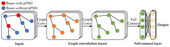
Figure 1.
GCN-based SR model for feature reconstruction.
2.1.1. Training Set
The training set of the GCN-based SR model comprises three parts: feature input matrix Xi, adjacent matrix A, and label matrix Yi, where is the number of features.
Each feature has its separate input matrix. The i-th input feature is expressed in a matrix Xi, where N represents the number of buses in the distribution network. As shown in the following equation, for key buses, their values in Xi are their real measurements. In addition, for buses that cannot be measured (no μPMU installed), their values in Xi are initialized using the adjacent key bus measurement and the KVL rule.
The topology of a distribution network with N buses is expressed in an adjacency matrix A, which indicates the connection relation between buses. As shown in the following equation, if is 1, it indicates that bus i and j are directly connected, while is 0 means they are not.
As shown in the following equation, the label matrix Yi corresponds to the input matrix Xi, which represents the real measurements of the i-th feature on the buses of the distribution network.
2.1.2. Structure Design
As a powerful deep-learning algorithm based on graph topology, the GCN has a strong nonlinear fitting ability for grid data. As shown in Figure 1, two graph convolution layers and one full connection layer comprise the SR model. The LeakyReLU function is selected as the activation function for graph convolution layers, as follows:
Based on the spectral graph theory, the output of the graph convolution layer can be formulated as follows [17]:
where and represent the output of the l + 1-th and l-th graph convolution layers. is the weight matrix, where Fh is the output dimension of the graph convolution layer. A is the adjacency matrix of distribution network topology. is the adjacency matrix with added self-connections, where I is the identity matrix. is the diagonal degree matrix of . is the activation function.
First, define , which describes the convolution process of the spectral graph. Then the output of the proposed GCN-based SR model can be formulated as follows:
where and are the weight matrix and bias matrix of the full connection layer.
The SR model is trained in a supervised manner, and the loss function consists of mean-square error (MSE) and Kullback–Leibler divergence loss (KLDivLoss) as follows:
2.2. Fault Classification and Location Via GNN
Since the distribution network topology is highly consistent with graph topology, GNN is very suitable for solving the problems in the distribution network. In this part, a special kind of GNN named GAT is adopted for fault classification and location tasks. As shown in Figure 2, the inputs of the model are feature estimates of all distribution network buses obtained by the SR model in the previous step. The inputs are first passed along to a fault classification model to obtain the fault type. Since most of the faults in the distribution network are single-phase faults, and since three-phase faults rarely occur [20], only single line-to-ground faults (SLG), line-line faults (LL), and double line to ground faults (LLG) are considered in this paper. In addition, it is set that the fault occurs on the buses, not the branches, because the data collected is the electrical features of the buses, which is determined by the installation position of μPMUs and can better reflect the fault information of the buses. Then, based on the fault type, inputs are passed along to the corresponding fault location model to obtain the label of the fault bus. In addition, the universal model for fault classification and location is illustrated in Figure 3, which consists of two graph attention layers and one full connection layer. Different color topologies in each layer represent different feature types.
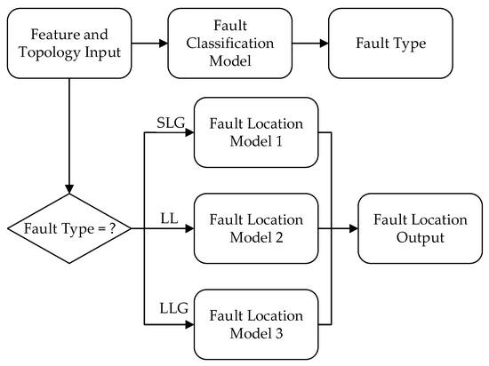
Figure 2.
Process for fault classification and location.
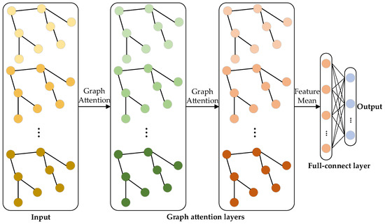
Figure 3.
GAT-based universal model for fault classification and location.
2.2.1. Training Set
The training set of the proposed fault classification and location model comprises three parts: input matrix X, adjacent matrix A and label y.
The input of the proposed fault classification and location model is the estimated values of all features of all distribution network buses obtained by the SR model in the previous step. It is expressed in an matrix X as follows, where N represents the number of buses and F represents the number of features.
The adjacent matrix A is the same as in the SR model in the previous step.
The label consists of two parts: fault classification label yc and fault location label yl. They are converted to one-hot vectors when calculating losses.
where n represents the number of fault types, which is 3 in this paper, and m represents the number of distribution network buses.
2.2.2. Structure Design
Define the input to graph attention layer as a set of bus features , where N represents the number of buses and F represents the number of features. The output of this layer is a new set of bus features whose feature dimension is F′, . An illustration of three-head attention (K = 3) by bus 1 on its adjacent bus is shown in Figure 4. Each attention computation is represented by a separate color. In addition, is obtained by averaging the aggregated features from each head. Then the output of the graph attention layer based on the multi-head attention mechanism can be expressed as [18]:
where || is the concatenation operator. is the activation function LeakyReLU in (4). K is the number of heads of the attention mechanism. is some neighborhood of bus i in the graph. are normalized attention coefficients computed by the k-th attention mechanism, and is the corresponding weight matrix.
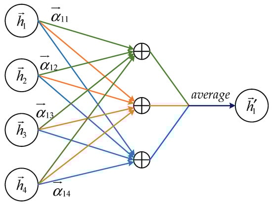
Figure 4.
An illustration of multi-head attention (with K = 3 heads) by bus 1 on its adjacent bus.
In this paper, as shown in Figure 5, a single-layer feedforward neural network with weight vector as parameters constitutes the attention mechanism a. Then the normalized attention coefficient can be computed by the attention mechanism as follows [18]:
where is the weight matrix.

Figure 5.
The attention mechanism a in this paper.
Then the output of fault classification and location model can be evaluated as follows:
where is the output of the i-th bus of the j-th graph attention layer. and are weight matrixes, where is the output dimension of the graph attention layer. Z is the output of the full connection layer. and are the weight matrix and bias matrix of the full connection layer, where No is the output dimension of the full connection layer.
The model is trained in a supervised manner, and the loss function is cross-entropy loss as follows:
where onehot (.) is the one-hot function.
3. Experiment and Discussion
In this section, we first test the performance of the proposed fault classification and location method in the IEEE 37 bus system. Then, the influence of noise, fault resistance, μPMUs allocation, DGs access, and network reconfiguration on the locating performance of this method are discussed.
3.1. IEEE 37 Bus Test Case
The IEEE 37 bus system, as shown in Figure 6, is utilized here for both simulation and experimental tests to validate the proposed method. Based on the definition of the key bus in Section 2.1, measurements are obtained from μPMUs installed at buses 702, 703, 704, 705, 707, 708, 709, 710, 711, 720, 734, 744, 799.
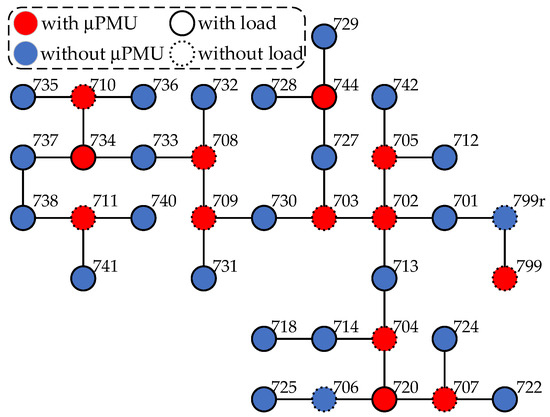
Figure 6.
IEEE 37 bus system for test.
Faults are simulated for all buses in the system based on OpenDSS software (Version 9.3.0.2). The default fault resistance is 10 Ω. The load level is randomly selected between 0.3 and 1. The voltage, current phasors, and powers are measured during the fault. We obtain the training and test datasets used for feature reconstruction and fault classification and location. A total of 50 data samples are generated for each fault type at each bus. As a result, the entire dataset contains 7400 data samples, which were divided into 80% training set and 20% test set.
Some feature reconstruction results based on the proposed SR method are shown in Figure 7. Table 1 evaluates the reconfiguration performance of each feature using Mean Absolute Percentage Error (MAPE) and coefficient of determination R2. It is shown that the proposed method has a good capability for distribution network feature reconstruction. Note that the R2 of voltage is not very high because of its large cardinal number. There is an overall offset between the reconstructed value and the real value, which does not affect the subsequent training. In addition, the average relative errors of the training set and test set are all less than 10% in experiments.
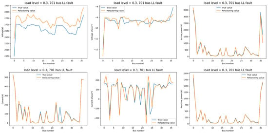
Figure 7.
Some feature reconstruction results based on the proposed SR method.

Table 1.
Reconfiguration performance of each feature.
The performances of the proposed method were visualized by the confusion matrix in Figure 8. It is shown that the average accuracy of the fault classification model is above 99%. The accuracy of the fault location model is 95.7%, and the erroneous location is mostly distributed near the fault bus.
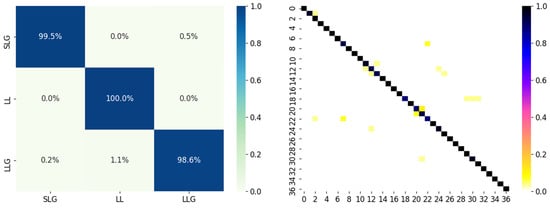
Figure 8.
Confusion matrix of performances of fault classification and location in IEEE 37 Bus system.
3.2. Influence of Fault Resistance
The proposed method is tested under various fault resistances in this part. Specifically, we chose fault resistances of 0.05 Ω, 10 Ω, 25 Ω, and 1000 Ω for the experiments. The fault location results are shown in Figure 9. Here we define a k-hop accuracy to represent the accuracy of the error locating bus within k hops Ω from the real fault bus, since the zero-hop accuracy is not satisfactory when the fault resistance is very small or large.

Figure 9.
Fault location results with different fault resistance.
The k-hop accuracy results for different fault resistances are indicated in Figure 9, and more numeric results are in Table 2. When the fault resistance is 10 Ω and 25 Ω, the zero-hop accuracy is above 95% and the three-hop accuracy can be more than 99%. However, when the fault resistance is 0.05 Ω and 1000 Ω, the zero-hop accuracies are about 70% and 60%, respectively, but the three-hop accuracy can still reach 90%, which indicates that the proposed model can still capture a part of the fault characteristics for these faults. The erroneous location is deemed to be affected by the parameters of lines. If the fault resistance is much smaller or larger than the adjacent line impedance, the location tends to be incorrect [15].
Table 2.
Comparison results with different fault resistance.
3.3. Influence of Noise
In practical application, measurements often contain noises generated by environmental factors [21]. In this part, the locating performance under noise of the proposed method is studied. We added 10 dB, 20 dB, 30 dB, and 40 dB Gaussian noise to the test set for the experiments. The location results are shown in Figure 10, and more numeric results are in Table 3.
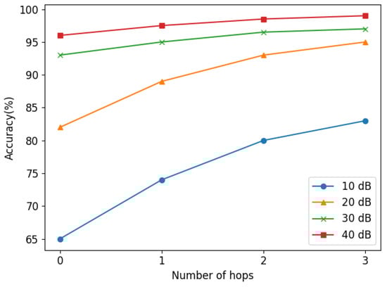
Figure 10.
Fault location results with different noise.
Table 3.
Comparison results with different noise.
It is shown that with the decrease in signal-to-noise rate (SNR), the locating performance of the proposed method decreases. However, when SNR is 30 dB and 40 dB, the zero-hop locating accuracy is above 92%. In addition, when SNR is 10 dB, the three-hop locating accuracy is still more than 83%, which indicates that the proposed fault location method is quite robust to mild noise. At present, the measurement error of μPMU is mostly below 1%. Thus, the anti-noise ability of the proposed method can meet most practical application scenarios.
3.4. Influence of the μPMU Allocation
In Section 2.1, key buses where μPMUs are allocated are defined. We installed μPMU on buses with more adjacent buses because more distribution network characteristic information can be obtained by doing so. Experiments in the IEEE 37 Bus system also prove the feasibility of this allocation method. In this part, two other allocation methods are tested for comparison with the method used in this paper: Allocation 1, to use the same amount of μPMUs as this paper used and allocate them into the distribution network at equal intervals; and Allocation 2, to install μPMUs directly on all the front and end buses of the distribution network (such as bus 799, 712, 725, etc. in IEEE 37 Bus system).
The numeric comparison results are shown in Table 4 and Figure 11 shows the k-hop fault location results. It is shown that the μPMU allocation used in this paper is superior to the other two methods. Among them, the performance of Allocation 1 is similar to that of the method in this paper, and the performance of Allocation 2 is the worst.
Table 4.
Comparison results of different μPMU allocations.
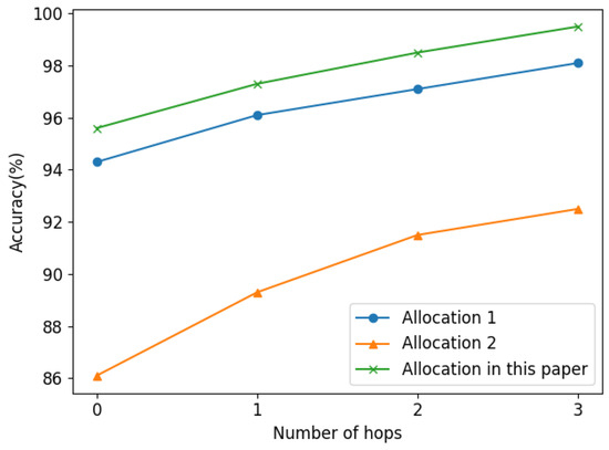
Figure 11.
Fault location results of different μPMU allocations.
3.5. Influence of Distribution Network Reconfiguration
To reduce loss or balance the loads, the configuration of a distribution network may change [22]. In this part, to assess the performance of the proposed method under distribution network reconfiguration, we modified the topology of the IEEE 37 Bus system and conducted experiments under the following three cases of reconfiguration:
- Disconnect bus 709 and bus 730 and connect bus 708 and bus 730;
- Disconnect bus 702 and bus 703 and connect bus 705 and bus 727;
- Disconnect bus 702 and bus 713 and connect bus 703 and bus 713.
The location results are shown in Figure 12, and more numeric comparison results are in Table 5. It is shown that the performance of the proposed method degrades somewhat due to the reconfiguration of the distribution network, which is deemed to be affected by the robustness of the proposed model and the position changes of the key buses after network reconfiguration. In addition, the closer the reconstructed network is to the original network, the better the performance of the proposed method is. However, the zero-hop locating accuracy and three-hop can still be above 85% and 90%. respectively. Note that the reconfiguration scenarios are not involved in the model training process, which means the proposed method is somewhat robust to distribution network reconfiguration.
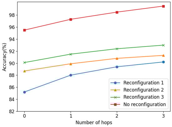
Figure 12.
Fault location results of different reconfigurations of the distribution network.
Table 5.
Comparison results of different reconfiguration of distribution network.
3.6. Influence of DGs Access
As a mushrooming number of DGs are connected to the distribution system, traditional fault location methods are challenged by distorted fault currents from DGs. In this part, we investigate the performance of the proposed method for distribution network with DGs access.
To simulate a multi-DGs condition, DGs are added at buses 718, 725, 735, and 741 in the IEEE 37 Bus system. Based on the definition of the key bus in Section 2.1, and based on the original allocation of μPMU in Section 3.1, μPMU should also be installed on the above bus connected to DG to better obtain the characteristic information from DGs. The numeric results are shown in Table 6, and Figure 13 shows the k-hop fault location results. It is shown that the performance of the proposed method degrades slightly with DG access. However, the zero-hop locating accuracy is still 92.3% and the three-hop accuracy can also be above 98%, which proves that the proposed method is somewhat robust to DG access.
Table 6.
Comparison results with DGs access.
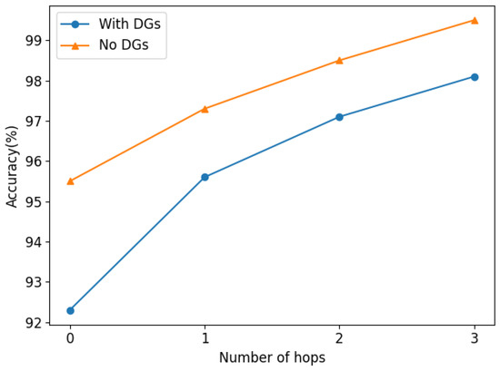
Figure 13.
Fault location results with DGs access.
3.7. Performance in Another Complex Distribution Network
As the previous experiments are all conducted in the IEEE 37 bus system, to verify the effectiveness of the proposed method in more complex distribution networks, we have tested it in the IEEE 123 bus system [23]. As in the IEEE 37 bus system, the fault measurement data of the key buses in the IEEE 123 bus system is obtained according to the definition of the key bus in Section 2.1, and then the proposed SR-GNN-based model is utilized to obtain the fault type and fault location.
The performance of the proposed method in the IEEE 123 bus system is shown as the confusion matrix in Figure 14. It can be proved that the proposed method can still achieve good performance in complex distribution networks such as the IEEE 123 bus system, since the average accuracy of the fault classification and location model are still above 98% and 95%, and the erroneous location is mostly distributed near the fault bus.
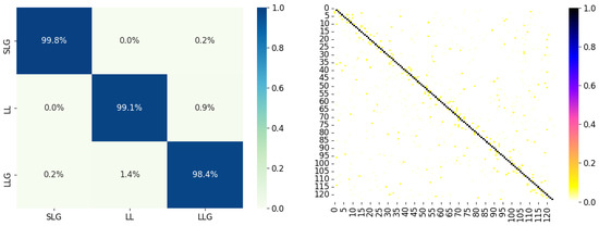
Figure 14.
Confusion matrix of performances of fault classification and location in IEEE 123 Bus system.
3.8. Performance Comparison with Existing Advanced Methods
To compare the performance of the proposed SR-GNN-based method with the existing fault location methods and to show that the proposed method has the current high identification accuracy and good economy, this section selects some advanced fault location methods proposed in the last two years and makes a comparison with the proposed method.
The results of the comparison are shown in Table 7. It is shown that, although using the SR model to reduce sensor cost, the fault location accuracy of the proposed method is still comparable to those of using wide area measurement methods. In addition, in the methods also using sparse measurement, it still has a slightly higher performance than some methods, such as the sparse voltage measurement-based method in [15], which proved that the proposed method can guarantee high positioning accuracy while having a good economy.
Table 7.
Comparison results with existing advanced methods.
4. Conclusions and Outlook
In this paper, we develop an SR-GNN-based fault classification and location method in the power distribution network. Unlike most methods that rely on wide area measurement, the proposed method can accurately evaluate the fault type and location only by obtaining the measurements of some key buses with μPMU in the distribution network. This reduces the construction cost of the distribution system. In addition, it is tested in IEEE 37 Bus system to verify its effectiveness. Further experiments show that the proposed method has a certain anti-noise capability and is robust to fault resistance change, distribution network reconfiguration, and distributed power access. In a nutshell, this paper proposes a high-performance and low-cost fault diagnosis and location method for the power distribution system.
The method proposed in this paper is a cloud intelligent algorithm and is deployed on the cloud platform of the distribution network. The cloud platform is typically a high-performance computer that can easily deploy the proposed method. After the data collected by the μPMUs on the distribution network buses is uploaded to the cloud platform, fault diagnosis can be performed. Therefore, the proposed method can be used by industry.
The main innovation points of this paper are as follows: (1) Based on sparse bus measurement, the SR method in the image processing field is utilized to estimate and reconstruct all bus features of the distribution network; (2) Using the model based on GAT for distribution network fault diagnosis.
Although the proposed method has good performance under most conditions, how to improve its fault diagnosis and location ability in some specific conditions, such as the detection of high impedance faults, remains to be further studied. In addition, this paper can inspire new guidelines for research, such as memristor based circuits [25] fault detection, and power flow calculation of distribution network.
Author Contributions
Conceptualization, Y.P. and H.M.; methodology, H.M.; software, H.M.; validation, Y.P., W.W. and H.M.; formal analysis, H.M.; investigation, H.M.; resources, W.X.; data curation, T.C.; writing—original draft preparation, H.M.; writing—review and editing, Y.P.; visualization, T.C.; supervision, W.W.; project administration, Y.P.; funding acquisition, W.X. All authors have read and agreed to the published version of the manuscript.
Funding
This research was funded by [National Key R&D Program of China] grant number [2020YFB0906000, 2020YFB0906002].
Data Availability Statement
The data are not publicly available due to restrictions privacy.
Conflicts of Interest
The authors declare no conflict of interest.
References
- Czarnecki, L.S.; Staroszczyk, Z. On-line measurement of equivalent parameters for harmonic frequencies of a power distribution system and load. IEEE Trans. Instrum. Meas. 1996, 45, 467–472. [Google Scholar] [CrossRef]
- Chen, K.; Hu, J.; Zhang, Y.; Yu, Z.; He, J. Fault Location in Power Distribution Systems via Deep Graph Convolutional Networks. IEEE J. Sel. Areas Commun. 2020, 38, 119–131. [Google Scholar] [CrossRef]
- Faiz, J.; Lotfi-fard, S.; Shahri, S.H. Prony-based optimal Bayes fault classification of overcurrent protection. IEEE Trans. Power Del. 2007, 22, 1326–1334. [Google Scholar] [CrossRef]
- Gill, P. Electrical Power Equipment Maintenance and Testing; CRC Press: Boca Raton, FL, USA, 2008. [Google Scholar]
- Lin, W.; Yang, C.; Lin, J.; Tsay, M. A fault classification method by RBF neural network with OLS learning procedure. IEEE Trans. Power Deliv. 2001, 16, 473–477. [Google Scholar] [CrossRef]
- Ferrero, A.; Sangiovanni, S.; Zappitelli, E. A fuzzy-set approach to fault-type identification in digital relaying. IEEE Trans. Power Deliv. 1995, 10, 169–175. [Google Scholar] [CrossRef]
- Zhang, Y.; Zhang, Y.; Wen, F.; Chung, C.Y.; Tseng, C.; Zhang, X.; Zeng, F.; Yuan, Y. A fuzzy Petri net based approach for fault diagnosis in power systems considering temporal constraints. Int. J. Electr. Power Energy Syst. 2016, 78, 215–224. [Google Scholar] [CrossRef]
- Youssef, O.A.S. Combined fuzzy-logic wavelet-based fault classification technique for power system relaying. IEEE Trans. Power Deliv. 2004, 19, 582–589. [Google Scholar] [CrossRef]
- Das, S.; Santoso, S. Distribution Fault-Locating Algorithms Using Current Only. IEEE Trans. Power Deliv. 2012, 27, 1144–1153. [Google Scholar] [CrossRef]
- Lotfifard, S.; Kezunovic, M.; Mousavi, M.J. Voltage Sag Data Utilization for Distribution Fault Location. IEEE Trans. Power Deliv. 2011, 26, 1239–1246. [Google Scholar] [CrossRef]
- Halab, N.E.; García-Gracia, M.; Borroy, J.; Villa, J.L. Current phase comparison pilot scheme for distributed generation networks protection. Appl. Energy 2011, 88, 4563–4569. [Google Scholar] [CrossRef]
- Shi, S.; Lei, A.; He, X.; Mirsaeidi, S.; Dong, X. Travelling wavesbased fault location scheme for feeders in power distribution network. J. Eng. 2018, 2018, 1326–1329. [Google Scholar]
- Guo, M.-F.; Gao, J.-H.; Shao, X.; Chen, D.-Y. Location of Single-Line-to-Ground Fault Using 1-D Convolutional Neural Network and Waveform Concatenation in Resonant Grounding Distribution Systems. IEEE Trans. Instrum. Meas. 2021, 70, 1–9. [Google Scholar] [CrossRef]
- Trindade, F.C.L.; Freitas, W.; Vieira, J.C.M. Fault location in distribution systems based on smart feeder meters. IEEE Trans. Power Del. 2014, 29, 251–260. [Google Scholar] [CrossRef]
- Jia, K.; Yang, B.; Dong, X.; Feng, T.; Bi, T.; Thomas, D.W.P. Sparse Voltage Measurement-Based Fault Location Using Intelligent Electronic Devices. IEEE Trans. Smart Grid 2020, 11, 48–60. [Google Scholar] [CrossRef]
- Pinte, B.; Quinlan, M.; Reinhard, K. Low voltage micro-phasor measurement unit (μPMU). In Proceedings of the 2015 IEEE Power and Energy Conference at Illinois (PECI), Champaign, IL, USA, 20–21 February 2015; pp. 1–4. [Google Scholar]
- Kipf, T.N.; Welling, M. Semi-Supervised Classification with Graph Convolutional Networks. arXiv 2016, arXiv:1609.02907. Available online: http://arxiv.org/abs/1609.02907 (accessed on 9 September 2016).
- Velickovic, P.; Cucurull, G.; Casanova, A.; Romero, A.; Lio, P.; Bengio, Y. Graph Attention Networks. arXiv 2017, arXiv:1710.10903. Available online: https://arxiv.org/abs/1710.10903 (accessed on 30 October 2017).
- Dugan, R.C.; McDermott, T.E. An open source platform for collaborating on smart grid research. In Proceedings of the 2011 IEEE Power and Energy Society General Meeting, Detroit, MI, USA, 24–28 July 2011; pp. 1–7. [Google Scholar]
- Wang, X.; Zhang, H.; Shi, F.; Wu, Q.; Terzija, V.; Xie, W.; Fang, C. Location of single phase to ground faults in distribution networks based on synchronous transients energy analysis. IEEE Trans. Smart Grid 2020, 11, 774–785. [Google Scholar] [CrossRef]
- Etezadi-Amoli, M.; Ghofrani, M.; Arabali, A. Performance of advanced meters: Effects of different temperatures and loading conditions on meter accuracy. In Proceedings of the 2014 IEEE/PES Transmission & Distribution Conference & Exposition (T&D), Chicago, IL, USA, 14–17 April 2014; pp. 1–5. [Google Scholar]
- Baran, M.E.; Wu, F.F. Network reconfiguration in distribution systems for loss reduction and load balancing. IEEE Trans. Power Del. 1989, 4, 1401–1407. [Google Scholar] [CrossRef]
- Kersting, W.H. Radial distribution test feeders. In Proceedings of the 2001 IEEE Power Engineering Society Winter Meeting. Conference Proceedings, Columbus, OH, USA, 7 August 2001; pp. 908–912. [Google Scholar]
- Zhang, Y.; Wang, J.; Khodayar, M.E. Graph-Based Faulted Line Identification Using Micro-PMU Data in Distribution Systems. IEEE Trans. Smart Grid 2020, 11, 3982–3992. [Google Scholar] [CrossRef]
- Buscarino, A.; Fortuna, L.; Frasca, M.; Gambuzza, L.V.; Sciuto, G. Memristive chaotic circuits based on cellular nonlinear networks. Int. J. Bifurc. Chaos 2012, 22, 1250070. [Google Scholar] [CrossRef]


Disclaimer/Publisher’s Note: The statements, opinions and data contained in all publications are solely those of the individual author(s) and contributor(s) and not of MDPI and/or the editor(s). MDPI and/or the editor(s) disclaim responsibility for any injury to people or property resulting from any ideas, methods, instructions or products referred to in the content. |
© 2022 by the authors. Licensee MDPI, Basel, Switzerland. This article is an open access article distributed under the terms and conditions of the Creative Commons Attribution (CC BY) license (https://creativecommons.org/licenses/by/4.0/).