Abstract
The intelligent and appropriate regulation of indoor temperatures within heritage buildings is crucial for achieving nearly Zero-Energy Building (nZEB) standards, since the technical improvement of the envelope and the overall shape of heritage buildings should be very limited in order to preserve the buildings’ authenticity. Thermal comfort is a very important factor that influences the energy performance of a building and the wellbeing of its end users. The present paper focuses on the development of a dynamic thermal human stress model that aimed to accurately predict the necessary garment insulation within a typical high-inertia heritage building. Two different statistical approaches (a Hoke D6 design and a composite factorial design) were employed for the development of this meta-model adapted to a typical mixed-mode heritage building seeking to obtain nZEB classification. Thermal human stress was modeled through the prediction of the thermal absorptivity (b) in accordance with the updated ASHRAE 55 model. Physically measured indoor climate parameters, outdoor meteorological data, and building operational information were coupled to the subjective sensorial dimensions of the problem with the aim of identifying the necessary garment insulation levels within heritage buildings composed of high-thermal-mass materials (for example, stone, concrete, and ceramic tiles). Our investigation focused on the parameter directly linked to the cold/warm sensations experienced due to clothing insulation: thermal absorptivity (b). In brief, the present paper proposes a third-order regression polynomial model that facilitates the calculation of thermal absorptivity, relying on adaptive thermal comfort concepts. The meta-model was then evaluated using Adrian Bejan’s constructal law after conducting entropy analysis. The constructal evaluation of the meta-model revealed the characteristic size of the domain regarding variable thermal absorptivity (b) and identified the necessary evolution of the model in order to increase its forecasting capacity. Thus, the model provided accurate forecasting for thermal absorptivity values greater than 50 Ws−1/2 m−2K and will be developed further to improve its absolute location accuracy for scenarios wherein the thermal absorptivity value is lower than 50 Ws−1/2 m−2K.
1. General Context, Findings, and Outcomes
Nowadays, thermal comfort research tends to involve multifaceted big data problems, since extremely large datasets may be analyzed computationally to reveal patterns, trends, and associations, especially relating to human behavior and interactions with indoor thermal environments. Furthermore, since we have to consider immeasurable occupants’ subjective experiences in relation to measurable thermodynamic physical parameters, the increased number of potential real-world scenarios has made thermal comfort assessment a very complex problem [1,2,3,4,5,6,7,8,9,10,11,12,13,14,15,16,17,18,19,20,21,22,23,24,25,26,27,28,29,30,31,32,33,34,35,36,37,38,39,40,41,42,43,44,45,46,47,48,49,50,51,52,53,54,55,56,57,58,59,60,61,62,63,64,65,66,67,68,69,70,71,72,73,74,75,76,77,78]. This explains why forecasts of thermal comfort models‘ output data may conflict even for the same data node and even if the model seems to have a satisfactory predictive capability. Therefore, this paper aims to accurately address the complexity of the problem by presenting a robust method for forecasting big data in relation to the thermal comfort of occupants in mixed-mode (MM) heritage buildings.
The research methodology took into account a large amount of prediction data during target data calculation to construct a big-data forecast garment insulation meta-model. First, the calculated data regarding thermal sensation were correlated with the most influential parameters using second-order polynomial equations. Additionally, the necessary conditions for the use of the proposed polynomial functions were analyzed. Then, an accurate polynomial function was identified, and the data thresholds that improved its forecast capacity were determined through the application of the constructal law [78]. Point-to-point comparison with a specific predictive model showed that the proposed polynomial model quickly forecast occupants’ thermal sensations in an MM heritage building. Finally, after the constructal evaluation of the different entropy measures of the standardized residuals, we identified the target entropy of our dataset in order to understand the model’s behavior within the range of our simulation domain.
In order to situate our interdisciplinary study within its general context, the paper was organized around several themes to provide readers with an accurate overview of the current and past research on the following five distinct sub-themes that are crucial for understanding the limits and importance of the research presented herein:
- Thermal comfort models and international standards;
- Thermal characteristics of fabrics and thermodynamic parameters;
- MM ventilation strategies and building operation;
- Design of Experience (DOE) methods and Response Surface Methodology (RSM);
- Constructal law and entropy analysis.
Case Study: Heritage Building and Nearly Zero-Energy Building (nZEB) Categorization, or Why Indoor Thermal Comfort Is a Crucial Factor for Overall Energy Performance
The intelligent and appropriate regulation of indoor temperatures within heritage buildings is crucial for achieving nZEB standards, since the technical improvement of the envelope and the overall shape of heritage buildings should be very limited. Thus, the main energy conservation strategy applied should optimize the use of the heating system, matching it to the real needs of the occupants and adjusting it to their garment insulation levels. Compared to uncontrolled use, the overall energy consumption could be reduced by at least 20% while also providing optimal thermal comfort conditions. Consequently, the present paper focuses on the proposal of a garment insulation forecasting meta-model that aimed to accurately predict the indoor thermal comfort conditions within a typical high-inertia heritage building. This model could be very useful in the renovation of heritage buildings, since it could be employed to program the heating and/or cooling HVAC systems in a way that reduces the overall energy consumption of the building.
The research presented here is timely, especially regarding the adaptation of heritage buildings to climate change. Any intervention carried out on a building of heritage interest must respect its character-defining elements, which may take the form of spatial configurations, appearance, building structure, and technical building systems. Any measure leading to the alteration of these elements should be avoided. The appropriate regulation of indoor thermal comfort using less energy is a non-destructive method for reducing the overall energy consumption of a building.
It is noteworthy that in general, interventions in heritage buildings must be additive and, as far as possible, non-invasive and reversible in order to minimize their impact on the heritage interest. Each building of heritage interest must be considered as a special case. The heritage interest of the building must be carefully assessed in light of its regional, national, and even international cultural context. Understanding the authenticity, integrity, and heritage interest of a building makes it possible to define the characteristic elements that should be preserved. The recommended measures must comply with the principles of building conservation defined in international charters and regulations.
Considering the risk of the trivialization and disappearance of a large portion of built heritage, architects and specialized engineers have proposed interventions seeking to optimally reconcile the objectives of increasing energy performance to meet the nZEB standards and preserving the heritage of the built environment. Additionally, the French Ministry of Culture officially supports actions committed to reconciling heritage conservation with energy performance and even energy-efficiency objectives targeting “nearly Zero-Energy Building” (nZEB) categorization for heritage buildings in the near future. In this context, studying the intrinsic qualities of a building of heritage interest is essential before beginning any project that targets nZEB categorization.
Hence, the research presented in this paper enhances this specific and sustainable approach that reflects a desire to preserve what is essential to a building, highlight its intrinsic qualities, and reuse or recycle as many materials as possible. Nevertheless, from an architectural point of view, we conducted this research on saving energy through the appropriate regulation of indoor thermal comfort in relation to garment insulation in order to avoid a systematic focus on the irremediable modification of facades, e.g., by installing insulation and other technical solutions from the outside, replacing all the windows and old joinery, and installing solar panels on the roof, without taking into account the heritage and landscape interest of the building.
Our approach combined the in-depth preliminary study of the building with thermal comfort optimization through the minimization of energy usage (focusing on thermal inertia and ventilation strategies) and could be coupled to complementary soft interventions such as the detection of thermal bridges, research into innovative solutions from a technical point of view, the use of materials and products that are durable and risk-free for the long-term conservation of structures, finishing works, and architectural decorations. Through appropriate studies, we should identify pragmatic solutions adapted to each building of heritage interest.
In a complementary manner, from an institutional point of view, actions have been taken in this direction within the framework of the production of specific European standards adapted to the conservation of cultural heritage. In June 2017, the NF EN 16 883 standard (entitled “Energy performance of buildings of heritage interest”) was published. This European standard—designed by heritage practitioners and building professionals (architects, engineers, etc.)—provides guidelines for improving the energy performance of buildings with historical, architectural, or cultural value in a sustainable manner while respecting their heritage interest.
The standard recommends a working procedure for the choice of measures based on the investigation, analysis, and documentation of the building and its indoor thermal comfort conditions and the assessment of the impact of the proposed measures in relation to the preservation of the characteristic architectonic elements of the building. The standard also underlines that the proper maintenance and operation of the heritage building is the best conservation measure. Any improvement measures must therefore facilitate the ongoing maintenance of the building and any added features and materials. The research presented in this paper focused on improving thermal comfort within heritage buildings and fully complied with the aforementioned NF EN 16 883 standard.
2. Introduction, Thematic Subjects, and Interdisciplinary Aspects
The notion of thermal comfort is not recent. Objective and measurable thermo-physical meteorological parameters such as temperature and relative humidity, along with subjective perceptual parameters such as comfort sensation, have been closely linked to energy efficiency and wellbeing in research and architectural production for some time. Claude Bernard initiated thermal comfort research in the 19th century, while the Kansas State University started working on the subject in the 1930s. However, the first world petrol crisis during the early 1960s intensified international research on thermal comfort [1]. Moreover, the industrial revolution of the nineteenth century and the consequent twentieth-century innovations in applied thermal, climatic, and mechanical engineering led to new physical and sensorial approaches to architectural spaces [1,2,3].
All these applied and theoretical approaches, as well as the generalized systemic vision established during the heyday of the thermodynamics discipline, also contributed to the domination of the modernist ambition to create “healthier” environments for future society. A characteristic example is the Athens Charter, which was published in 1933 by the famous Swiss architect Le Corbusier [4,5]. This theoretical text was one of the most influential documents on urban planning in the history of architecture and was based on urban studies undertaken by the 4th International Congress of Modern Architecture (Congrès International d’Architecture Moderne—CIAM) held in Athens in the early 1930s. For the first time, minimum qualitative thresholds were introduced regarding the required amount of solar exposure equally meted out between all dwellings, while an hygienic vision of architecture was theorized by coupling modern techniques and scientific achievements to construct tall apartment buildings that were widely spaced to provide optimal air quality and free up the soil for large green parks in order to improve wellbeing and sensorial spatialization [4,5]. From then on, architectural design became more wellbeing-sensitive, since this document represented the first time that architectural theory had linked spatialization to sensation and comfort. Even though this approach gradually led to a purely quantitative vision of these optimized parameters and tended to reduce the subjective dimensions of wellbeing and comfort, we can assume that it changed our conceptions of space.
Following this, although the postmodern movement ignored and/or underestimated the impact of architecture on the natural environment, the contemporary environmental crisis, which first appeared in the nineteen sixties with the global petrol crisis, led to the integration of many technological achievements into architectural discourse and practice from different points of view. For example, many performance indexes have been institutionally introduced in order to evaluate architectural production, while the first ad hoc administrative vademecums on this subject appeared during the nineteen sixties in the form of thermal regulations. This led the architectural and research community to adopt a global approach that focuses on the predictive quantitative evaluation of architectural design. Thus, issues that were explored qualitatively until the nineteen thirties, such as sunlight, natural ventilation, CO2 concentration, and odors, are now quantified; hence, in order to be built, a well-conceived building must satisfy strict ad hoc quantitative dynamic standards that evolve over time [1,6]. This explains why, during the late twentieth and, in particular, twenty-first century, many quantitative studies focused on sunlight and thermal energy consumption in the building sector.
Nevertheless, as previously mentioned, this was also the natural evolution of the circumstances wherein the modernists qualitatively treated sunlight as an agent of cultural, medical, and technological change in the early nineteen thirties [7,8,9]. Similarly, regarding concerns about CO2 concentration and odors, hygienic issues highlighting the necessity of introducing clean and open air into indoor environments date back to the late eighteenth century, when the industrial revolution was globalized. These hygienic parameters linked to architectural spatialization appeared for the first time in the form of an architectural manifest in the Athens Charter [4,5,6,7,8,9].
Subsequently, the general notion of comfort was introduced into the field of scientific research in the early 1930s, “when psychology and behavioural sciences decided to define themselves as natural sciences as long as they started operating between the purviews of two distinct dreadful edges: the world of the cultural institutional framework that regulates the mechanisms of understanding, ideation and credence, and on the other hand, the omnipotent torrent of natural phenomena” [10] cited in [11,20] (p. 9). Nevertheless, the first thermal comfort models appeared in the late 1960s, while Fanger’s comfort equation™ was established by P.O. Fanger in 1970s [12]. Fanger’s mathematical formalization was significant, as it represented the first generalized approach involving the quantitative combination of environmental and individual variables in a minimalist manner. Fanger introduced the Predicted Mean Vote (PMV) index as a result of his comfort equation [11,12]. Through this parameter, one could obtain information on how occupants judge an indoor thermal environment. Following this, many new comfort models were proposed, while international thermal comfort standards were established to optimize the thermal acceptability of indoor thermal environments [11,12,13,14,15,16,17,18,19,20,21,22,23,24,25,26].
In the present paper, a novel predictive polynomial thermal comfort model that focuses on clothing-related thermal sensation (from the perspective of human physiology) is proposed. Human skin temperature changes as a result of blood-flow regulation in the skin, and it is an important physiological parameter of thermal comfort that has not been previously studied in the manner presented in this paper, wherein resides the originality and the novelty of the present work. Changes in human skin temperature, which one could consider in close connection to the concept of clothing-related thermal sensation, were regarded in this study as the parameter that influences heat transfer between the human body and the environment and a human stress response to cold or heat, since skin temperature has an effect on human thermal sensation, and clothing significantly influences skin temperature. The model was therefore based on the statistical creation of a fictive dataset that was constructed using a recently updated thermal comfort equation proposed by Kim et al. [28,29]. Kim et al.’s equation included and correlated the most influential subjective and measurable parameters, while its mathematical formalistic expression followed the updated ASHRAE 55 pattern [13].
The purpose of our approach was to explore the wide range potential combinations and propose a sufficiently robust thermal comfort quantitative forecasting model for a typical mixed-mode-interior heritage building, with the aim of linking the subjective occupant-experience dimension to clothing insulation thermal characteristics and meteorological data. In order to obtain the final polynomial mathematical formulation, many scenarios were constructed on the basis of distinct Design of Experiments (DOE) methods. Thus, a training dataset of parameters was established with the use of two distinct DOE methods, and each proposed model was evaluated over a randomly constructed test dataset for both DOE designs in order to identify the most robust forecasting model with satisfactory predictive capabilities. Finally, beyond the quantitative aspects of our study, we aimed to understand and address how clothing insulation thermal characteristics in a mixed-mode heritage building (MM) that integrates both natural and mechanical ventilation strategies may influence occupants’ thermal comfort perceptions, as well as how this method should evolve over time in order to provide more robust results.
3. State of the Art
According to Fanger’s theory, as reported in his textbook or in the ASHRAE handbook of fundamentals [12], the parameters to be considered are four physical (air temperature, air velocity, relative humidity, and mean radiant temperature) and two subjective (“personal”) parameters (metabolic rate and clothing insulation). Outdoor meteorological conditions are only considered in adaptive thermal comfort models, mainly in terms of outdoor running temperature (see also de Dear’s studies [11,20,21]). The level of thermal insulation provided by garments is one of the most important thermal comfort parameters, since adequate clothing may significantly reduce the optimum operative temperature and, consequently, the building’s energy consumption impact. Studying thermal comfort management in relation to subjective and measurable parameters with the aim of optimizing indoor thermal environments is a complex and multifaceted problem, since the human thermoregulatory system is much more convoluted than any existing natural or artificial control system due to its concatenation and synchronous operation of a gargantuan array of regulatory mechanisms.
Thermal comfort evaluation becomes a much more complicated problem when one considers heritage buildings that are aiming to obtain nZEB certification while operating in mixed mode (MM) as a substitute for consolidated HVAC for both comfort [11,12,13,14,15,16,17,18,19,20,21,22,23,24,25,26,27,28,29] and energy efficiency [28,29]. This complexity arises because the indoor environment of an MM heritage building is not fully controlled, and so the occupants’ subjective experiences are very important in the assessment of thermal comfort conditions, since both natural and mechanical ventilation strategies are closely and implicitly related to the outdoor meteorological conditions. However, contemporary research has demonstrated concretely that even though it is much more complicated to evaluate indoor thermal comfort in such conditions, by employing an appropriate design and operation strategy, MM buildings can improve comfort and energy performance, especially in Mediterranean, humid subtropical, and warm temperate moist forest climates [28,29,30,31,32,33,34,35,36,37,38,39,40,41,42,43,44]. Nevertheless, even though it has been proven that MM designs can offer many advantages in regulating indoor thermal environments, there is increasing international debate on the optimal thermal comfort thresholds at the interface of the two modes of operation in such buildings [28].
Furthermore, as is easily understandable, the thermal properties of textile fabrics are of considerable concern and relevance for thermal comfort research [45,46,47,48,49,50,51], since an occupant’s overall thermal comfort perception is significantly influenced [11,12,13,14,15,16,17,18,19,20,21,22,23,24,25,26,27] by the variations in their mean skin temperature due to the thermophysical properties of their clothing, as explicitly cited in the ISO 9920 (see also [45,46,47]). Additionally, the development of the fabric industry over the last 50 years has led to the introduction of new materials that contribute significantly to the total heat transfer between the skin and garments [45,46,47]. Nowadays, fabrics are considered to be highly porous media, and new parameters that influence their thermal identity have been introduced. More precisely, contemporary post-fabrication treatments, such as textile surface curing and sophisticated finishing processes, inevitably influence the thermal characteristics of a garment [45]. Hence, recent textile research has investigated the thermal parameters through which we can observe and quantify the influence of in-vogue materials on a garment’s thermal characteristics [45,46,47,48,49,50,51].
3.1. Thermal Comfort Theories and Related International Standards
The ASHRAE 55 American standard defines thermal comfort as “…a subjective concept related to physical and psychological well-being in agreement with the environment” [13] cited in [11] (p. 10). This indicates that the notion of thermal comfort involves several distinct optimum parameters and necessitates complex transdisciplinary study [11]. Concretely, in order to assess the thermal comfort of an individual, a variety of factors and parameters that impact the heat transfer process between the human body and its surrounding environment must be studied. Furthermore, psychosomatic parameters also come into play, since human beings are unique entities with a variety of multicultural sensorial experiences.
Past research has revealed that the ratio of produced to exchanged heat between the human body and its immediate environment automatically varies in an endless, repeated, and regular manner [12,20]. This happens because the human thermoregulatory system is in a continuous process of achieving thermal equilibrium. For this reason, when Fanger studied the human thermoregulatory system [12,20] in the early 1980s, he introduced a complex systemic approach that involved investigating the body as a complex system of heat generation that is continuously autoregulated in a dynamic relationship with its surrounding environment.
Thus, as thermal engineers/designers, our main research task is to provide an indoor thermal equilibrium. In such a scenario, indoor thermal comfort is reached by achieving thermally neutral conditions. In thermodynamic terms, applied thermal engineering in buildings aims to design indoor environments that can offer stable thermal conditions and reduce the continuous heat transfer between the human body and its surrounding environment. Therefore, a compromise between internal temperatures (ranging from the central neural system’s temperature to other deep body temperatures), skin temperatures, and the indoor temperature has to be reached [11,12,20]. This target is very difficult to achieve, since one must determine a variety of measurable and immeasurable parameters, and the temperature fluctuations in the surrounding environment also influence the human body’s perceptions [11,12,13,14,15,16,17,18,19,20,21,22,23,24,25,26,27,28,29]. The human thermoregulatory system is very sensitive to microclimate variations and rapidly thermally adapts to anticipate variations in indoor microclimatic conditions [11,12,13,14,15,16,17,18,19,20,21,22,23,24,25,26,27,28,29].
Note that the aforementioned thermal autoregulatory system is not identical for every human being and depends on a variety of cultural and biological idiosyncrasies. Additionally, complementary behavioral thermoregulatory mechanisms supplement this metabolic thermoregulatory system. These mechanisms are directly associated with subjective comfort or discomfort sensations, whereas control actions include changing the performed activity, altering the system’s operation, or continuously re-adjusting one’s clothing insulation [11,12,13,14,15,16,17,18,19,20,21,22,23,24,25,26,27,28,29].
Past research has focused on suggesting general objective frameworks for studying and evaluating the subjective issue of thermal comfort [11,12,13,14,15,16,17,18,19,20,21,22,23,24,25,26,27,28,29]. This explains why a variety of models, thresholds, and indexes are nowadays available to be applied to indoor thermal comfort assessment, showing the need for a concise global quantification methodology. According to past research [11,12,13,14,15,16,17,18,19,20,21,22,23,24,25,26,27,28,29], the most influential parameters in regard to thermal comfort are the following:
- The local air velocity, which influences the heat exchange between the body and the surrounding environment via convection due to changes in the evaporation on the skin’s surface. Convection is heat transfer via the bulk movement of molecules within fluids such as gases and liquids, including molten rock (rheid). Convection includes sub-mechanisms of advection (the directional bulk-flow transfer of heat) and diffusion (the non-directional transfer of energy or mass particles along a concentration gradient). Air velocity affects heat transfer due to the temperature difference between the air and body surfaces and also promotes evaporation from the skin. In MM buildings, this parameter is very important, especially when the building operates in natural ventilation mode in order to avoid local discomfort issues. In order to ensure thermally comfortable conditions, we should generally limit the indoor air velocity to around 0.2–0.3 m/s.
- Clothing insulation, which refers to the resistance to heat transfer between the two boundaries of the skin’s surface and the surrounding environment (all details are explicitly presented in ISO 9920, see also [45,46,47]).
- The ambient air temperature and the surficial wall temperature, which directly influence thermal comfort. The “cold wall” effect refers to the cold feeling experienced when an occupant stands near the elements of the building envelope (walls or windows). This occurs because the temperature of these elements is significantly lower than that of ambient air.
- Metabolism, i.e., the biological thermoregulatory process (thermal body homeostasis) that regulates the internal heat of the human body; for healthy organisms, the internal temperature at the skin level is maintained around 36.6 °C.
- The air’s relative humidity, i.e., the ratio of the partial pressure of water vapor to the equilibrium vapor pressure of water at the same temperature. Studies have revealed that humid air transmits sensations of cold or heat much more effectively than dry air because it contains water vapor (see also [45,46,47]).
In order to determine a subjective method for assessing the degree of thermal discomfort among building users, sophisticated experiments involving human subjects have been conducted [11,12,13,14,15,16,17,18,19,20,21,22,23,24,25,26,27]. Many different approaches and theories have been formulated, while several international standards have been established in order to define a common framework for robust thermal comfort forecasting and evaluation. In order to understand how we can merge occupants’ subjective experiences and measurable parameters in a single quantitative model, we will now focus on the most widely accepted theories and then briefly review the main international standards related to thermal comfort in terms of the approaches/theories adopted.
3.1.1. The Concept of Koestel and Tuve [14]
In the mid-1950s, Koestel and Tuve [14] focused on the evaluation of the air’s velocity and temperature within a specific indoor environment and tried to mathematically assess the influence of these parameters on an occupant’s thermal sensations. They made an important assumption that may have invalidated their results: infrared radiation and relative humidity were considered to be constant. Thus, considering that the human body is immersed within an ever-changing environment, wherein the air velocity and temperature change in a constant manner, they proposed a mathematical formulation to quantify the temperature difference between any point in the occupied zone and the control conditions, introducing the concept of the Effective Draft Temperature (EDT) to demystify the feelings of coolness or warmth in any area of the human body at the skin level.
3.1.2. Fanger’s PMV and PPD Concepts [12,15]
During the late 1970s, Ole Fanger introduced a human-centered transdisciplinary approach (applied thermodynamics, psychophysics, ergonomics, architecture, textile engineering, and thermal physiology) to study the problem of thermal comfort assessment [15]. Aiming to propose a mathematical forecasting relation, Fanger derived an original Comfort EquationTM, introducing two original indexes, Predicted Mean Vote (PMV) and Predicted Percentage of Dissatisfied (PPD). The combination of these two indexes was expected to be capable of predicting the optimal indoor thermally comfortable conditions. Fanger’s indexes represented an update on the Effective Draft Temperature (EDT) concept by taking into consideration the three modes of heat transfer (radiation, conduction, and convection), as well as metabolic mechanisms such as respiration and perspiration. The output of Fanger’s calculations was the Predicted Mean Vote (PMV) index, which, according to his theory, could forecast the potential thermal vote of a number of occupants located within the studied indoor conditions [12,15]. To improve the predictive capacity of the model, he introduced a complementary index named Predicted Percent of Dissatisfaction (PPD) to complement the PMV [12,15]. The PPD index predicted the percentage of occupants in discomfort. Fanger’s PMV index expressed the average thermal sensation experienced by a large group of individuals based on the wide thermal sensation scale proposed by ASHRAE, and a value of 10% for the PPD index corresponded to a value between −0.5 and +0.5 for the PMV index [11,12,15,20].
3.1.3. Gagge’s Two-Node Model and the Updated Effective Temperature (ET) Concept [16,17,20]
During the late 1970s, at the same time Fanger was introducing his PPD and PMV indexes, Gagge et al. [16,17] revisited a simple concept that was introduced in the early 1920s by Houghten and Yaglou [18]. These authors proposed the Effective Temperature (ET) index, taking into consideration three important comfort parameters: air temperature, air velocity, and relative humidity [18,20]. Subsequently, Gagge et al. presented the hypothesis that the human body comprises only two layers, the core and the skin, and on this basis, they developed the Pierce two-node model to overcome steady-state theories by lending a dynamic dimension to the notion of thermal comfort, since Fanger’s approach approximated only statical steady-state conditions [11,12,15,20].
This approach was a direct consequence of Gagge’s past research. Gagge et al. [16,17] tried to integrate into the ET approach the influence of the metabolic rate and clothing, and so the ET index was developed into a corrected Effective Temperature (ET*) index and a corresponding Effective Temperature Scale (SET*) index. However, this initial approach was also a steady-state method, and for this reason, Gagge et al. followed the current of the 1970s that established a common scientific vision that “for any given combinations of metabolic rate, surrounding environment and clothing there exist a theoretically determined equilibrium core temperature and an associated skin temperature” [17] cited in [10,11] (p. 16).
Gagge et al.’s Pierce two-node model [16,17] introduced the nodal thermophysiological approach to thermal comfort research [11,20]. This concept resulted in a transient dynamic model that forecast physiological variables under unsteady transient conditions [11,16,17,20]. The direct outputs of the Pierce two-node model were skin temperature and skin wetness, and these parameters were used to calculate the SET* index introduced by Gagge et al. [16,17]. Note that this approach opened up new paths for the thermophysiological description of thermal comfort, since it explained all the metabolic thermoregulatory mechanisms in terms of thermal signals from the core, the skin, and the body, while the human body was modeled as two concentric compartments representing the center of the body and the skin layer [11,16,17,20].
3.1.4. The Berkeley Model [19]
With the passing of time, Fanger’s model was revealed to be insufficient to efficiently predict thermal comfort conditions within non-homogeneous and transitional environments [19,20]. In order to improve upon the steady-state approaches and introduce a transient thermodynamic dimension to the problem, nodal thermophysiological theories were developed based on Gagge’s approach [16,17]. The main differences between the various nodal thermophysical models were the ways in which the appropriate thermal comfort indexes under warm or cold environments were calculated, as well as the significant increases in the number of nodes, body segments, and layers that divided the human body to provide a more detailed physical description of the problem. Among these complex contemporary models, the Berkeley model proposed by Huizenga et al., the model proposed by Fiala, and the Stolwijk-like models are the most frequently used in the field [19,20]. The Berkeley model is quite sophisticated, since it takes into consideration all the parameters influencing thermal comfort (metabolic rate, clothing, air temperature, mean radiant temperature, air velocity, relative humidity, contact surface thermal properties, and physiological constants) and employs an unlimited number of sequential sets of environmental and physiological input conditions, defined as phases [19]. The Berkeley approach introduced into thermal comfort studies the Computational Fluid Dynamics (CFD) theory by modeling the human geometry, defining a precise mesh, and setting the boundary conditions according to the environmental parameter to solve the heat transfer balance equations using finite-difference (or sometimes a control volume) spatial discretization [19,20].
3.1.5. Adaptive Thermal Comfort Concept
The adaptive thermal comfort concept is an alternative approach that was mainly developed due to the increasing criticism of the static perspective of Fanger’s approach and the fact that the solely rational approaches generally neglected the sociocultural dimension of thermal comfort [11,20,21]. Adaptive thermal comfort models are merely empirical equations that correlate acceptable operative temperature (indoor) with exponentially averaged outdoor temperatures; on the contrary, the Berkeley model is a complex model of thermoregulation. According to de Dear et al. [21,22], the reasons that the rational thermal comfort models that did not consider the user’s subjectivity had limited applicability were that they adopted a steady-state perspective and were not validated on the basis of real-world field studies, since they did not take into account the sociocultural dimension of the problem.
Thus, the adaptive approach introduced field study research and underlined three different levels of investigation: physiological, psychological, and behavior adaptation [21]. Subsequently, according to the adaptive concept, databases were introduced into thermal comfort research. The creation of databases increased our knowledge of the prevailing optimum thermal conditions in different building types that are regulated under different protocols and for different climates and regions. Through statistical correlations generated by sophisticated data analysis methods, different models could be proposed for specific occupational scenarios and building operation types. Additionally, the systemic approach was introduced in a clearly transient heat transfer problem, since objective measurable parameters were studied in close relation to immeasurable subjective responses that were codified on the classic ASHRAE scale. These two dimensions of the problem are merged in statistical forecasting models that are applied only in specific conditions and environments and are being constantly improved.
Finally, this approach reinvented the abstract linear causality of the previous physiological–analytical approaches (heat transfer mechanisms/physiology/thermal comfort) [20,21,22]. The radical element of the adaptive thermal comfort concept was that it provided a holistic vision in comparison to the solely physiological or analytical approaches, wherein specific environmental conditions were imposed on individuals in laboratory conditions (individual climate chambers) [20,21,22]. Previous research considered prefabricated comfort conditions that did not take into account the interactivity of the occupants and their ability to act within the environmental conditions setup [20,21,22].
Thus, although these approaches enriched our understanding in the past, they are no longer in use, since they consistently underestimated the subjective dimension of comfort. Current international standards (such as the updated version of ASHRAE 55) are based on the classic analytical approach; nevertheless, the statistical exploitation of databases resulted in the development of a series of alternative algorithms that are applied to specific climatic types, operational protocols, and occupant scenarios to account for adaptation [11,20,21,22]. For this reason, among all the presented approaches, the present study adopted the adaptive thermal comfort concept to develop a statistical regression model that links measurable and subjective parameters in the case of an MM heritage building.
3.1.6. International Standards and Databases
Nowadays, there are three principal commonly accepted ISO documents that define precise methods of measurement for evaluating and assessing thermal comfort within moderate and extreme thermal environments: EN ISO 7243: 2017 (EN ISO 7243, 1989) [23]; EN ISO 7933 (EN ISO 7933, 2004) [24]; and ISO 11079 (EN ISO 11079, 2007) [25]. Additionally, even though its operability is limited, the classic EN ISO 7730 (EN ISO 7730, 2004) [26] standard reproduces Fanger’s approach and is built on the associated thermal comfort equation. Furthermore, according to Nicol and Wilson [22], the updated EN 15251 international standard, which linked thermal comfort to a building’s overall energy performance through the definition of internal desirable thermal comfort conditions, was retired and replaced by EN 16798-1 and EN 16798-2.
Finally, the well-cited and most common operational protocol, the ASHRAE 55 thermal comfort standard, was updated “with the desideratum to provide a well-validated method for thermal comfort assessment respectively correlating the degree of local and global satisfaction to the level of clothing and activity” ([13], cited in [11,20] (p. 18)). The employed concept was based on Fanger’s PMV–PPD index in conjunction with the SET* concept using a holistic adaptive approach ([13], cited in [11,20]). Finally, de Dear developed a global database of thermal comfort field experiments: the freely accessible RP-884 database [11,20,21]. The statistical regression model presented in this paper was built on an approximate thermal comfort model developed according to a database similar to the RP-884-database for MM heritage buildings.
3.2. Thermodynamic Properties of Clothing (ISO 9920)
As explained in the previous subsection, clothing insulation was one of the most important parameters to include in our study. The elementary function of garments in relation to thermal comfort is determined through the thermal properties of the textiles [27,45,46,47,48,49,50,51]. Past textile research mainly focused on the measurement of textiles’ thermal properties, such as thermal conductivity, thermal resistance, and thermal diffusion, under steady-state conditions [45,46,47,48,49,50,51].
Furthermore, the influence of the type of weave and finishing on a fabric’s thermal properties has also been well-documented, revealing that the understanding of fabrics’ thermal performance is a very complicated problem; nevertheless, the subjective sensorial experience of the user depends on the way that he/she feels the garment at the skin level [45,46,47,48,49,50,51].
Thus, even if one has access to a technical datasheet detailing each fabric’s thermophysical characteristics, it is quite difficult to forecast and assess the thermal feeling of the fabric, since there are many parameters that influence thermal sensation. Additionally, the development of sophisticated methods for fabric finishing (for example, enzymatic desizing and the removal of warp size material before weaving, resin treatment by the PAD-DRY-FIX method, enzymatic treatment, ennoblement elastomeric finishing, and starch finishing) has increased this difficulty, since the influence of the finishing method is not necessarily assessed during the measurement of thermal indexes [45]. Even if the values before and after finishing vary, the thermal feeling of the fabric at the skin level cannot be predicted and estimated in an accurate way.
Thus, in the present study, we focused on the definition of an index called thermal absorptivity (which can also be found in the literature as thermal absorption). This index was introduced by Hes [47,48] as an indirect measure of the warm/cool sensation of textiles. Kawabata and Yoneda [46], during the 1980s, underlined the significance of the so-called warm/cool feeling in the determination of the end-user’s thermal comfort. According to Hes [47,48], thermal absorptivity determines the contact temperature of two bodies. Concretely, thermal absorptivity is a property of a fabric that informs us whether a user feels warm or cool at the first brief contact between the fabric and human skin [45].
Consequently, in this study, we used this index in relation to the clothing insulation parameter of our global indoor thermal comfort model for MM heritage buildings, taking advantage of the fact that thermal absorptivity does not depend on the conditions of the experiment and is directly related to other thermal properties, such as thermal conductivity and diffusion [45,46,47,48]. Hence, this parameter is also indirectly influenced by the finishing of the fabric as well as the thickness and density of the textile, and so it links the thermophysical characteristics of the material to the thermal sensorial experience of the user.
3.3. MM Building Operation
As we saw in Section 3.1, the occupants’ thermal comfort is directly linked to the operation protocol of the building. In this study, we focused on MM building operation for multiple reasons. The MM approach as a ventilation strategy offers clear benefits regarding air renewal and indoor air quality, since one can combine natural and mechanical elements in order to provide an optimal indoor thermal environment [28,29]. However, there is ambiguity regarding the thermal comfort targets under the two different modes of operation (natural and mechanical ventilation) [28,29].
This is also revealed by the existence of a variety of international standards and operating protocols. Many studies, for example, have developed original control strategies that were conceived to motorize window-opening schedules with the aim of reducing the heating or cooling load [30]. Sultana et al. [30] explicitly quantified the potential of the MM approach to reduce the cooling load during the summer period, showing that “10 to 20% savings on cooling loads could be achieved when decisions are made based on Hybrid Ventilation with fixed schedules and more than 65% savings when variable schedules strategies are applied” [30] (p. 7).
Nevertheless, ambiguity remained regarding the thermal comfort models that had to be included in the simulation input. Kim et al. [28,29] reported significant differences between the various international standards. For example, the European Standard EN 15251 was retired and replaced by EN 16798-1 and -2 [32], which allow the application of the dynamic adaptive thermal comfort model to MM buildings when natural ventilation (NV) is chosen as the main free-running ventilation mode. In contrast, the current updated version of ASHRAE Standard 55 [13] restricts the use of the adaptive thermal comfort model exclusively to natural ventilation (NV) spaces.
Thus, according to Kim et al. [28,29], the paradox remains that the rest of the MM building has to be treated as an exclusively air-conditioned (AC) space. A direct consequence of this is that the classic PMV–PPD static steady-state models must be applied even if the building is naturally ventilated. As we saw earlier in Section 3.1, the PMV–PPD approach is very limited, since it cannot capture the transient characteristics of the multifaceted thermal comfort problem and the subjectivity of the occupant. This also means that ASHRAE Standard 55 guides us away from the traditional passive approaches that significantly contribute to reductions in thermal energy consumption for space heating and cooling in the building sector.
Similarly, in New Zealand, the Green Star criteria for thermal comfort in office buildings do not promote natural ventilation strategies and encourage “the use of mechanical ventilation over natural ventilation which results in designers opting for air conditioning systems in office designs” [33] (p. 1). Notwithstanding, Rasheed et al. [33] concluded that it is a matter of urgency to encourage, through ad hoc, well-documented, and sufficiently evaluated regulatory protocols, the use of natural ventilation in office environments by designers, engineers, architects, and building owners.
Nonetheless, previous research has proved that the mode of operation undoubtedly influences an occupant’s thermal comfort [33,34,35,36,37,38,39,40,41,42,43,44]. Thus, many researchers have also proposed the application of the adaptive thermal comfort concept for MM buildings when NV is the chosen ventilation strategy [28,29,30,31,32,33,34,35,36,37,38,39,40,41,42,43,44].
Our longitudinal study was also located in this general context and developed a thermal comfort model that correlates the thermodynamic characteristics of clothing to meteorological parameters for MM heritage buildings. As has been previously shown, an occupant needs to interact with the indoor environment according to his/her thermal sensations. These “thermal feelings” are the immediate result of his/her clothing insulation.
Hence, we aimed in this study to correlate garment characteristics and, consequently, thermal comfort to the ever-changing indoor thermal environment via the mixed-mode strategy, since natural ventilation contributes significantly to changes in indoor thermal conditions and thus to occupants’ overall thermal perceptions. Likewise, we tried to show that natural ventilation remains a very interesting passive strategy for MM buildings, while thermal sensation can by subjectively moderated through clothing insulation optimization in order to avoid perceptions of thermal discomfort.
3.4. Design of Experience (DOE) Methods and Response Surface Methodology
Since we had access to a huge domain of data and an infinite number of potential scenarios, we applied Design of Experience (DOE) methods in order to construct a statistical regression model. To this end, response surface methodology (RSM) was applied. RSM is a common approach used in engineering and industrial design to conduct variance analysis and optimization or construct simple polynomial predictive models [58,59,60,61,62,63,64,65,66,67,68].
In our case study, simple factorial simulation plans were designed to identify a set of optimum simulation scenarios, and our research was conducted with the aims of: (a) identifying the interaction between the selected parameters and thermal comfort, and (b) determining the relationship between the variable of interest, y (thermal absorptivity), and the four variables, xi, referring to the main parameters that, according to the updated ASHRAE 55 international standard [13], influence thermal comfort.
Thus, we employed RSM to define a valid polynomial function in the form of y = f(xi), where y is considered the response (thermal absorptivity) and xi represents the variables investigated in each set of simulations (fabric density, thickness, and thermal capacity and minimum outside temperature). According to the RSM approach, the values of xi were the coordinates of a simulation point inside our investigated domain, and y was the calculated value of the response at that specific point. To calculate y, we used the ASHRAE 55 [13] adaptive thermal comfort model updated by Kim et al. [28]. In the past, we successfully employed DOE methods and RSM to:
- Identify and propose an empirical polynomial equation for calculating the overall thermal resistance of a complex sophisticated dynamic composite building envelope element departing from the in-wall air-gap thickness values [59];
- Reduce a complex numerical transient heat-transfer model to simple regression models in the form of polynomial equations, providing a robust polynomial function that could be used during the early design stages to forecast a composite envelope’s thermal performance [58,60];
- Develop accurate regression models for daylight factor prediction within buildings at an early design stage, when the relevant data have not been precisely determined (dimension of glazing area, materials, opacities) [61];
- Link wide-ranging geometrical and non-geometrical glazing options for daylight effectiveness estimation at an early design stage [62].
Other researchers have used these methods in a variety of complex problems, including: robust parameter design [63], the design of products that are resistant to the environment [64], the fast prediction of heating energy demand [65], the investigation of the impact of the building form on the overall energy consumption [66], and the prediction of monthly heating demand for residential buildings [67].
Thus, the main aim of our study was to model clothing thermal absorptivity responses through a regression polynomial equation that was able to calculate and immediately forecast all the responses for a given dataset of the identified parameters that fell inside the established thresholds of our field of study.
4. Materials and Methods
According to de Dear [20,21,28], the fundamental concept behind the adaptive comfort model suggests that the perception of thermal comfort is affected by the occupant’s past and current thermal experiences. The present study was based on field measurements collected by Kim et al. [28] and, in particular, the empirical regression model proposed by these authors to examine how participants’ thermal sensations change according to indoor temperature variations due to MM buildings’ operating protocols.
The novelty of our research lay in the fact that we included the fabric characteristics in order to calculate the change in human skin temperature, thus formulating a new model based on the updated ASHRAE 55 model [13] proposed by Kim et al. [28]. The fabric characteristics used in our regression model were explicitly discussed in Section 3.2 and may significantly influence thermal sensation, especially inside MM heritage buildings with high thermal inertia at the envelope level.
Mathematical Formulation of the Problem
Kim et al. [28] recently developed a novel thermal comfort model after processing a huge dataset compiled from a longitudinal field experiment. In this study, the data collection was conducted in a mixed-mode-ventilation building, and the model combined observed data (such as physically measured indoor parameters, building operational information, and outdoor meteorological data) and subjective parameters (such as occupant thermal comfort) [28,29].
Kim et al. [28] concluded that different modes of building operation, such as natural or mechanical ventilation, significantly affect the subjective perception of an indoor thermal environment, while occupants seem to be more tolerant and adaptive to indoor thermal conditions when the building solely operates in the natural ventilation mode. The main output of Kim et al.’s study [28] was an improved ASHRAE Standard 55 clo model [13]. The ASHRAE Standard 55 presented a dynamic clothing insulation (Icl, in clo) predictive model in relation to the outdoor temperature at 6 a.m. according to the research findings of Schiavon and Lee [27]. The mathematical formulation of this approach was as follows ([13,27] cited in [28]):
where Icl (in clo) is dynamic clothing insulation, and Tout6a.m. is the measured outside temperature at 6 a.m. The R-squared value of this predictive model was 0.33. According to their observed values, Kim et al. [28] found that the ASHRAE model underestimated the clo value when Tout6a.m. < 18 °C and overestimated the clo value when Tout6a.m. > 18 °C. Nevertheless, Kim et al. [28] detected up to a few degrees (°C) of inconsistency between ToutMIN and Tout6a.m. and proposed an improved version of the ASHRAE Standard 55 model. Their predictive model was built in relation to the outside daily minimum air temperature, ToutMIN, instead of Tout6a.m.. This model had a very high R-squared value of 0.37 [28] and was formulated mathematically as follows:
However, as we have already theoretically established, dynamic clothing insulation can also be calculated from the following equation:
where Rclothing is the overall thermal resistance of the fabric. The thermal resistance of a fabric (Rclothing) is connected mathematically to the fabric thickness σ (in m) and thermal conductivity k (in Wm−1K−1) through the following equation [46]:
From Equations (3) and (4), we obtain:
In order to introduce into our model the subjective sensation and the objective measured parameters of the fabric, we employed the parameter of thermal absorptivity (b) [45,47,48]. Thermal absorptivity (b, in Ws1/2m−2K) is a surface property that changes based on the use of the fabric (laundry, wear, ageing) and the finishing processes. This parameter was of interest in our study since it allows the assessment of the fabric characteristics in terms of “cool-warm” sensations, according to Frydrych et al. [45] and Hes et al. [47,48]. Specifically, fabrics with a low value of thermal absorptivity (b) provide a “warm” feeling, according to Hes et al. [47,48]. The finishing of a fabric also significantly influences the thermal absorptivity parameter. It has been observed and reported that elastomeric finishing produces lower thermal absorptivity values and, consequently, warmer sensations than starch finishing [45,46,47,48,49,50,51]. As a rule of thumb, according to the literature [45,46,47,48,49,50,51], fabrics with a regular, flat, and smooth surface have a high thermal absorptivity value, offering a cooler sensation, while fabrics of lower regularity and smoothness and higher surface roughness have a lower b value, offering a warmer feeling. The parameter of thermal absorptivity (b) was calculated according to the following relation [45,47,48]:
where k is the thermal conductivity in Wm−1K−1, ρ is the volumetric fabric density in kg/m3, and cp is the specific heat capacity of the fabric in Jkg−1K−1. Thus, developing Equation (6), we obtain:
After combining Equations (5) and (7), we obtain:
Or, employing the equation of Kim et al. [28], we obtain:
Equation (9) correlates the cool/warm feeling of a fabric to the fabric characteristics and the minimum observed outside temperature through the value of thermal absorptivity.
5. Results and Discussion
The evaluation of the regression models was based on a point-to-point comparison between the output of Kim et al.’s equations [28] and the statistical-model-predicted values of thermal absorptivity. In our case study, none of the expected outcomes (fabric thermal absorptivity) varied in a linear manner according to the selected variables (fabric thermal capacity, minimum observed outdoor temperature, and fabric thickness and density). Considering that all the control factors had a qualitative dimension [69], in order to enable the quantification of the predicted responses, two different DOE methods were used: a central composite plan and a Hoke D6 design.
In both cases, the responses could be modeled in a quadratic manner [69]. For this reason, in order to include in our problem the sensory influence of the fabric’s thermal capacity, the minimum observed outdoor temperature, and the thickness and density of the fabric, we converted the general equation introduced, among others, by Box and Jones [64], Parker [69], Lucas [70], and Myers et al. [71] into:
where xi is the value of the ith factor (i = 1, 2, 3, …), and xj is the value of the jth factor (j = 1, 2, 3, …). The parameters were carefully selected to produce a composite factorial design and a Hoke D6 design, whereby, as in our past research [58,59,60,61,62], the effect of each factor was evaluated at three different levels (two for the investigation and one for the validation of the statistical model) according to codified values of −1, 0, +1. In order to cover an extremely large domain of potential scenarios and extend the applicability of our polynomial function, the thickness of the fabric ranged between 0.00002 m and 0.007 m, while the median value was equal to 0.0350 m.
The three investigated fabric density values were 500 kg/m3, 750 kg/m3, and 1000 kg/m3, while the fabric thermal capacity values were 1000 J/kg K, 1500 J/kg K, and 2000 J/kg K.
Finally, the three investigated minimum outside temperatures (T) were 5 °C, 15.45 °C, and 25.9 °C. Thus, according to the problem’s characteristics, in both DOE designs, the variance function of the fabric thermal absorptivity (b) in the simulation domain [−1, 1] was as follows:
For the thermal absorptivity (b) outcome, the values obtained were the root mean square error (RMSE), the scale-free normalized RMSE, and the standardized residuals, while the verification scores were derived using the contingency approach [70,71,72,73,74,75,76,77]. The RMSE and the scale-free normalized RMSE were calculated according to the following equations [70,71,72,73,74,75,76,77]:
In the equations above, M represents the polynomial regression model results, and O represents the results of Kim et al.’s model [28]. In our problem, we implemented a dataset built using the applied DOE method. Then, according to the employed DOE method, we performed regression on this first training dataset and obtained a polynomial equation. Afterwards, we constructed a separate test dataset, which was randomly created by selecting values that fell within the simulation domain.
Subsequently, we tested the regression on this second test dataset. Then, we calculated the root mean square error (RMSE) on both the training and test data. Since there exist no RMSE thresholds by which we could determine whether our polynomial model had a high forecast capacity, we calculated the normalized RMSE (NRMSE). Normalizing the RMSE (obtaining the NRMSE) by dividing it by the standard deviation was very useful, as it provided a scale-free RMSE value that could, for instance, be transformed into a percentage through Equation (13).
The NRMSEs for our training and test datasets should have been similar if our regression model was robust enough and had a satisfactory forecasting potential. If the NRMSE of the test set was much higher than that of the training set, it was likely that the model badly overfit the data.
If the NRMSE of the test set was much lower than that of the training set, it was likely that the model badly underfit the data. In general, for both cases, the models tested well in the sample, but the composite factorial model had a poor predictive value when tested out of the sample. Thus, in our case study, the model resulting from the Hoke D6 design was the best model, in the sense that it:
- Provided us a good in-sample fit, associated with low error measurements and normalized residuals (NMRSE for training data, −0.406478699; NMRSE for test data, −1.417656707).
- Avoided systematic random overfitting and slightly underfit the data by providing us a satisfactory out-of-sample forecast accuracy.
Finally, we also calculated the standardized residual ratio. The standardized residual was the difference between the output of the ASHRAE 55 [13] model updated by Kim et al. [28] and the expected count calculated by our polynomial function, divided by the standard deviation of the expected count. A general rule for understanding and interpreting the standardized residual is:
- When the residual is less than −2, the model’s output is less than the expected output.
- When the residual is greater than 2, the model’s output is greater than the expected output.
Actually, the standardized residual is a measure of the difference between observed and expected values, and in general it ranges between −2 and 2. It acted as an indirect measure of the significance of our model’s output according to the chi-square value.
When we compared the different scenarios, the standardized residual made it easy to determine which scenarios contributed the most to the value, and which contributed the least.
Furthermore, we employed the standardization technique because it works even when the variables are not normally distributed, as was the case in our study [71,72,73,74,75,76,77]. The mathematical formula used to calculate the standardized residual (sRe) was as follows [71,72,73,74,75,76,77]:
The goodness-of-fit results for the two polynomial regression models are illustrated in Figure 1, Figure 2, Figure 3 and Figure 4. We can see that the Hoke D6 regression model achieved a satisfactory fit to the numerical model’s data trends and a very good fit to the absolute location (Figure 1, Figure 2, Figure 3 and Figure 4), while the composite factorial plans produced a solution that presented a good data fit for the training scenarios (Figure 1 and Figure 2) but a very poor forecasting capacity according to the test scenarios (Figure 3 and Figure 4).
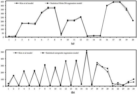
Figure 1.
Test dataset comparison. Both DOE methods provided models with satisfactory data trends and good fit to absolute location for the test datasets. (a) Outputs of Hoke D6 design model compared to those of Kim et al.’s model [28]; (b) outputs of composite factorial regression model compared to those of Kim et al.’s model [28]. y axis—b in Ws1/2 m−2K; x axis—the number of the tested scenario.
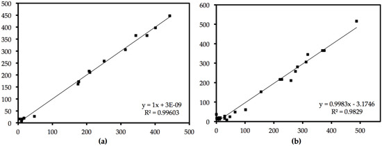
Figure 2.
Training dataset comparison. Least-square line equation and the square of the linear correlation coefficient are also shown for (a) Hoke D6 design and (b) composite factorial design. Both axes represent b in Ws1/2 m−2K.
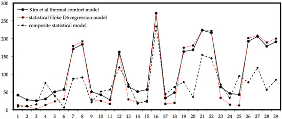
Figure 3.
Test dataset comparison. Hoke D6 design model’s satisfactory fit to Kim et al.’s model [28]: data trends followed the pattern of Kim et al.’s model. We can also observe from this graph the poor forecast capacity of the composite factorial plan regression model, since it presented a very bad fit to the absolute location and did not follow the data trends and the pattern outlined by Kim et al.’s model. y axis—b in Ws1/2 m−2K; x axis—the number of the tested scenario.
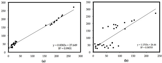
Figure 4.
Test dataset comparison. Least-square line equation and the square of the linear correlation coefficient are also shown for (a) Hoke D6 design and (b) composite factorial design. Both axes represent b in Ws1/2 m−2K.
Thus, as we saw in Figure 2, for the training scenarios, both models had high R2 values: 0.99603 for the Hoke D6 model and 0.9829 for the composite factorial regression model.
Nevertheless, in Figure 3 and Figure 4, we can observe that during the test scenarios, the Hoke D6 design responded more accurately and forecast far more effectively the thermal absorptivity (b).
Even though it underestimated some values, it represented with satisfactory fidelity the patterns and data trends and flawlessly predicted the higher and lower picks, with R2 = 0.9901. On the other hand, for the test scenarios, the composite factorial regression model was revealed to have a very poor forecast capacity.
In Figure 3, we saw that the composite factorial regression model did not follow the data trends, and in many places, we observed a pick inversion. This is better illustrated in Figure 4 and through the R2 value of 0.58705 for the testing scenarios. We observed a decrease of around 40% in the accuracy of the model. Thus, the Hoke D6 design performed better for our case study, and Equation (11) took the following mathematical form after the incorporation of the calculated coefficients:
It is very important to clarify at this stage that this regression equation aimed to provide a direct link between the outdoor minimum temperature and thermal absorptivity (b). Through the parameter of thermal absorptivity (b), we aimed to model the change in human skin temperature (as was explained in the section on the state of the art). From the perspective of physiology, this change is the result of skin blood-flow regulation, and it is an important physiological parameter of thermal comfort that has not been explicitly studied in the past; therefore, there exist no models that directly link thermal absorptivity (b) and climatic conditions, wherein resides the novelty of the present regression model. The change in human skin temperature, which we proposed to calculate using the parameter of thermal absorptivity (b), contributed a regression model that predicted the necessary level of garment insulation based on the heat transfer between the human body and the environment and forecast the human stress response to cold or heat. Finally, in order to use this Hoke D6 regression model through Equation (15), it was necessary to codify the values. The transformation of the equations from real values to codified values is presented in Figure 5, where y is the codified value of each parameter, and x is the real value of this parameter.
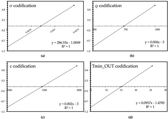
Figure 5.
Codification equations for each parameter. Each parameter had to be codified before using the regression equation that resulted from the Hoke D6 simulation scenarios. y axis—codified values; x axis—real values for (a) fabric thickness σ, (b) fabric density ρ, (c) fabric thermal capacity cp, and (d) minimum outside temperature Tout_min.
5.1. Analysis of Standardized Residuals’ Entropy
Let us now consider our Hoke D6 regression model as a complex thermodynamic system. As we know, in statistical mechanics, the robustness of any defined system can be found by calculating its entropy, which is defined as the system’s degree of disorder or, more specifically, the number of microstates the system possesses [57]. In our case, since we had an infinite number of potential scenarios within our simulation domain, we also had an infinite number of possible microstates for our system. The number of these states was determined using the well-known Boltzmann equation through the calculation of the target entropy S (in J/K) in relation to the possible microstates W and the Boltzmann constant kb [57], which is obtained by the general equation:
The interpretation of entropy applied in our case study could be controversial. Our interpretation of entropy was more philosophical. For us, entropy illustrated the degree of robustness of the Hoke D6 regression model. Robustness, in our case, did not mean that the model could calculate accurate and precise values. Since we dealt with thermal comfort and subjectivity, in our case, robustness implied that the regression model was dynamic and had the ability to vary within our simulation domain with and without restrictions or constraints, while still following the patterns, data trends, and picks of the original model that it reproduced.
Thus, in our case, W was the value of the standardized residuals, which illustrated the distance between the original model and our model. When we tried to calculate analytically the entropy (S) using the Equations (14) and (16), we obtained the following equation:
Furthermore, if we also combined Equations (9), (10) and (16) for the analytical expression of M and O, we obtained the following scheme:
Thus, to analyze S, we passed through the graphic representation of the standardized residuals. Considering the whole domain of the study, the graphical distribution of the overall standardized residuals, the trendline, and the R2 values are shown in Figure 6. We observe in Figure 6 that the residuals were generally distributed around a 6th-order polynomial trend. This 6th-order polynomial equation represented the potential number of microstates.
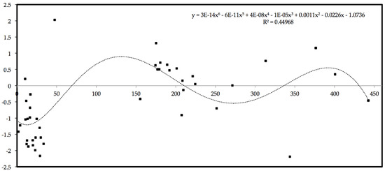
Figure 6.
Graphical distribution of the overall standardized residuals, trendline, and R2 values. x axis—b in Ws1/2 m−2K; y axis—entropy in J/K.
Due to the different errors that could exist because of the imperfection of Kim et al.’s model and the Hoke D6 regression model, a residual for a specific scenario had the tendency to gravitate around this 6th-order polynomial equation. Thus, to simplify Equation (17), we calculated S, employing the trendline equation instead of the analytical expressions, and we obtained the graphic representation of entropy shown in Figure 7.
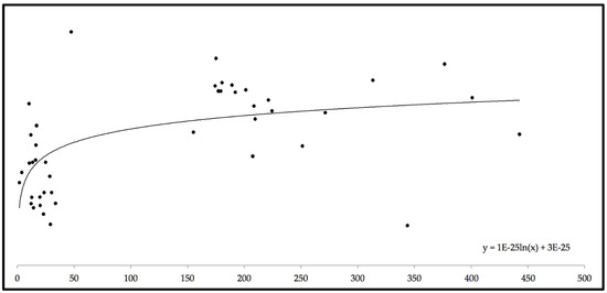
Figure 7.
Graphical distribution of the overall entropy and trendline. x axis—b in Ws1/2 m−2K; y axis—entropy in J/K.
In Figure 7, we can observe that the entropy of our system had a tendency to increase according to a logarithmic relation. Consequently, our predictive system could not robustly forecast in terms of absolute location very small values of thermal absorptivity (b) situated in the lower region of the data distribution (<50), since the entropy was not yet stabilized; thus, our system was in a state of total disorder. However, the entropy of our system tended to be constant for values of b that were higher than 50. This meant that the robustness and predictive capacity of our model were quite high for these values. This was also seen in Figure 1, Figure 2, Figure 3 and Figure 4. In particular, in Figure 3, we saw that the Hoke D6 regression model, even though it correctly represented the patterns, continuously underfit the absolute locations for values < 50. Figure 7 explains why this happened—within this range of values, the entropy of our system increased logarithmically, and so the disorder of our system dominated. Outside this range of values, the entropy of our system tended to be stable, and so, for this reason, the predictive capacity of our model provided greater accuracy for thermal absorptivity (b).
5.2. Constructal Evaluation and Evolution of the Hoke D6 Regression Model
Let us now consider that our Hoke D6 regression model was the product of a specific flow design that consisted of an irreversible complex thermodynamic flow system. To explain how the regression model flow system generated its configuration over time, we used the constructal law [78]. The constructal law is “universally valid, as physics, precisely because it is not a statement of static optimality and final design” [78] (p. 061003-6). In order to identify the most robust final equation, we used diverse mechanisms (factorial composite design and Hoke D6 design). Thus, the proposed equation was not our final design or the best design; rather, it represented the beginning of an original design that will evolve over time. According to the constructal law, optimization, maximization, and minimization are static notions regarding end designs; however, in real life, end and optimum design do not truly exist, according to Bejan [78], due to the direction of the evolution of time and the fact that design by nature is not static but dynamic and ever-changing [78]. Hence, for our problem, the proposed equation needed to evolve in order to improve the absolute location accuracy for scenarios wherein the thermal absorptivity is less than 50 Ws−1/2m−2K. Thus, we had to find a way to create scenarios that could train our model to freely achieve maximum fitness and adaptability, even though these two objectives are contradictory, local, and disunited [78].
We now address the dimension of the characteristic size of our model, which, in our case, was the size of the simulation domain. As we identified, our system evolved towards a maximum value of potential internal entropy generation. Even though natural systems have a tendency towards lower entropy generation, in our case, the system tended towards the maximum value of entropy and then stabilized around this value (Figure 6). However, even though the entropy was not minimized under these steady conditions, our system had a high forecast capacity (in terms of data trends and absolute location). Since our system seemed to have reached a first equilibrium state, the second stage was that the system had to form and evolve in order to minimize its internal entropy.
Contradictorily, when the system had lower entropy values, it presented more disorder, and when the entropy tended to be constant, the system performed better. Thus, our system was in the initial phase, and as disorder is caused by entropy fluctuation, the absolute value of entropy was not very important at this stage. In order to obtain a system that will perform better in the future, we have to identify a way to minimize the entropy value in a steady manner. If we transposed our problem into a pure thermodynamic problem (for example, an engine), we would observe that larger is better, because the component poses less resistance to the flow of fluid, heat, mass, and stress [78]. This is why larger values of thermal absorptivity present less internal entropy fluctuation, which is a natural tendency of all systems in order to initially facilitate flow and reduce the brake.
Nevertheless, the constructal law shows that in many applications smaller is better [78]. This, according to Bejan, is in conflict with the first hypothesis, “and from this conflict emerges the notion—the prediction, the purely theoretical discovery—that the component should have a characteristic size that is finite, not too large, not too small” [78] (p. 061003-5). Even though the model provided more accurate predictions for some scenarios, in general, it remains an amalgam of imperfect components. Thus, the future direction of our work is to identify a characteristic size for our simulation domain that would provide more effective statistical predictions in order to update our model and improve its accuracy for a larger range of values. The fact that we chose a huge domain of potential values significantly increased the number of scenarios, and so the model was not very accurate in the calculation of the variables located inside the extreme minimum thresholds of our simulation domain.
6. Conclusions
This work was premised on a conceptual framework combining features of statistical approaches and a recently developed adaptive thermal comfort model [28] that was built on the basis of longitudinal field studies. The index used to identify and characterize indoor thermal comfort was thermal absorptivity (b) according to the level of clothing insulation.
Comparing two different DOE methods, we identified that the Hoke D6 design provided scenarios with which we could develop a better polynomial regression model that could be used to robustly predict thermal absorptivity in relation to measurable meteorological data and garment characteristics for MM heritage building applications. The concept of “better” is used here in “physics terms, along with direction, design, and evolution” according to the constructal law [78] (p. 061003-6). Finally, a detailed error analysis was conducted, and the entropy of the standardized residuals was calculated in order to investigate the distance between the model-predicted data and reality. The Hoke-D6-resulting model provided us with good in-sample fit, associated with low error measurements and normalized residuals (NMRSE for training data, −0.406478699; NMRSE for test data, −1.417656707); avoided systematic random overfitting; and slightly underfit the data by presenting satisfactory out-of-sample forecast accuracy. In order to minimize the disorder of our predictive system, we now need to identify a more effective component to develop our model.
Thus, the future direction of this work is to identify the optimally equilibrated size for our simulation domain in order to improve the accuracy of our polynomial model in terms of absolute locations. Nevertheless, even in its present form, this study presented a new, sufficiently robust, adaptive thermal comfort model that improved in a complementary manner the ASHRAE 55 model. This model could be implemented in dynamic building energy simulation software, such as EnergyPlus, to improve the accuracy of the overall thermal energy performance forecasting of typical MM heritage buildings, with the purpose of calculating the thermal insulation and operational improvements necessary for obtaining the nZEB label.
Funding
This research received no direct external funding. Nevertheless, the research conducted in the framework of the present paper was produced in the context of the Erasmus+ e-CREHA Program (agreement no. 2020-1-NL01-KA203-064610) of the European Union, which supports innovation and creativity exploring the impact of climate change on heritage architecture. However, the European Commission and the Dutch National Research Agency cannot be held responsible for any use that may be made of the information contained herein.
Data Availability Statement
Data analyzed in this study were a re-analysis of existing data, which are partially included in Kim et al. (2019) [28]. New data have been produced according the scenarios presented in Kim et al. (2019) [28]. The statistical model simulations upon which this study is based are too large to archive or to transfer. Instead, we provide all the information needed to replicate the statistical simulations (Hoke D6 & composite factorial models). The model and the namelist settings are explicitly explained and available within the manuscript. Due to confidentiality agreements, supporting data can only be made available to bona fide researchers subject to a non-disclosure agreement.
Conflicts of Interest
The author declares no conflict of interest.
References
- Requena-Ruiz, I. Building Artificial Climates. Thermal control and comfort in Modern Architecture (1930–1960). Ambiances Environ. Sensib. Archit. Espace Urbain 2016, 2. [Google Scholar] [CrossRef]
- Gallo, E. Modern Movement Architecture and Heating Innovations in France 1900–1939. In Docomomo Technology Seminar. Climate and Building Physics in the Modern Movement; Tomlow, J., Wederbrunn, O., Eds.; DOCOMOMO: Löbau, Germany, 2008; pp. 91–96. [Google Scholar]
- Cooper, G. Air-Conditioning America: Engineers and the Controlled Environment, 1900–1960; John Hopkins University Press: Baltimore, MD, USA, 1998. [Google Scholar]
- Corbusier, L. Rétablir les conditions de nature. In Espaces Verts et Jardins; Eyrolles: Paris, France, 1957; Volume 7, pp. 33–43. (In French) [Google Scholar]
- Corbusier, L. La Ville Radieuse: Eléments d’une Doctrine D’urbanisme Pour L’équipement de la Civilisation Machinist; Vincent et Fréal: Paris, France, 1964. (In French) [Google Scholar]
- Farish, M. Creating Cold War Climates. The Laboratoires of American Globalism. In Environmental Histories of the Cold War; McNeill, J.R., Unger, C.R., Eds.; Cambridge University Press: New York, NY, USA, 2013; pp. 51–85. [Google Scholar]
- Daniel, S. Grille Climatique, 1951. In Le Corbusier Plans; Echelle-1 & Fondation Le Corbusier: Paris, France, 2005; Volume 11. (In French) [Google Scholar]
- Hobday, R. The Light Revolution: Health, Architecture, and the Sun; Findhorn Press: Forres, UK, 2006. [Google Scholar]
- Campbell, M. What Tuberculosis Did for Modernism: The Influence of a Curative Environment on Modernist Design and Architecture. Med. Hist. 2005, 49, 463–488. [Google Scholar] [CrossRef] [PubMed]
- Kantor, J.R. The nature of psychology as a natural science. Acta Psychol. 1939, 4, 1–61. [Google Scholar] [CrossRef]
- Mavromatidis, L. Unit 6. Thermal Comfort in Buildings. In Zero 001—Design and Optimization of Zero Energy Consumption Buildings—Using Innovative Methods of Distance Learning; National Kapodistrian University of Athens: Athens, Greece, 2016; p. 26. [Google Scholar]
- Ambrosio Alfano, F.R.; Olesen, B.W.; Palella, B.I. Povl Ole Fanger’s Impact Ten Years Later. Energy Build. 2017, 152, 243–249. [Google Scholar] [CrossRef]
- ANSI/ASHRAE Standard 55-2017; Thermal Environmental Conditions for Human Occupancy. ASHRAE: Atlanta, GA, USA, 2017.
- Koestel, A.; Tuve, G.L. Performance and evaluation of room air distribution systems. ASHRAE Trans. 1955, 61, 533. [Google Scholar]
- Fanger, P.O.; Pedersen, C.J.K. Discomfort due to air velocities in spaces. In Proceedings of the Meeting of Commissions B1, B2, E1 and the IIR, 4, Belgrade, Serbia, 16–18 November 1977. [Google Scholar]
- Gagge, A.P. Rational temperature indices of man’s thermal environment and their use with a 2-node model of his temperature regulation. In Federation of American Societies for Experimental Biology, Federation Proceedings; 1973; pp. 1572–1582. Available online: https://pubmed.ncbi.nlm.nih.gov/4705203/ (accessed on 9 December 2022).
- Gagge, A.P.; Fobelets, A.P.; Berglund, L.G. A standard predictive index of human response to the thermal environment. ASHRAE Trans. 1986, 92, 709–731. [Google Scholar]
- Houghten, F.C.; Yaglou, C.P. Determining lines of equal comfort. ASHVE Trans. 1923, 29, 163–175. [Google Scholar]
- Huizenga, C.; Hui, Z.; Arens, A. A model of human physiology and comfort for assessing complex thermal environments. Build. Environ. 2001, 36, 691–699. [Google Scholar] [CrossRef]
- Croitoru, C.; Nastase, I.; Bode, F.; Meslem, A.; Dogeanu, A. Thermal comfort models for indoor spaces and vehicles—Current capabilities and future perspectives. Renew. Sustain. Energy Rev. 2015, 44, 304–318. [Google Scholar] [CrossRef]
- de Dear, R.J.; Brager, G.S. Towards an adaptive model of thermal comfort and preference. ASHRAE Trans. 1998, 104, 145–167. [Google Scholar]
- Nicol, J.F.; Wilson, M. A critique of European Standard EN 15251: Strengths, weaknesses and lessons for future standards. Build. Res. Inf. 2011, 39, 183–193. [Google Scholar] [CrossRef]
- EN ISO 11079; Ergonomics of the Thermal Environment—Determination and Interpretation of Cold Stress when Using Required Clothing Insulation (IREQ) and Local Cooling Effects. International Standards Organization: Geneva, Switzerland, 2007.
- EN ISO 7243; Hot Environments—Estimation of the Heat Stress on Working Man, Based on the WBGT-Index (Wet Bulb Globe Temperature). International Standards Organization: Geneva, Switzerland, 1989.
- EN ISO 7730; Ergonomics of the Thermal Environment. Analytical Determination and Interpretation of Thermal Comfort Using Calculation of the PMV and PPD Indices and Local Thermal Comfort Criteria. International Standards Organization: Geneva, Switzerland, 2004.
- EN ISO 7933; Ergonomics of the Thermal Environment—Analytical Determination and Interpretation of Heat Stress Using Calculation of the Predicted Heat Strain. International Standards Organization: Geneva, Switzerland, 2004.
- Schiavon, S.; Lee, K.H. Dynamic predictive clothing insulation models based on outdoor air and indoor operative temperatures. Build. Environ. 2013, 59, 250–260. [Google Scholar] [CrossRef]
- Kim, J.; de Dear, R.; Tartarini, F.; Parkinson, T.; Cooper, P. Ventilation mode effect on thermal comfort in a mixed-mode building. In Proceedings of the IAQVEC 2019, Bari, Italy, 5–7 September 2019. [Google Scholar]
- Kim, J.; Tartarini, F.; Parkinson, T.; Cooper, P.; de Dear, R. Thermal comfort in a mixed-mode building: Are occupants more adaptive? Energy Build. 2019, 203, 109436-1–109436-11. [Google Scholar] [CrossRef]
- Sultana, S.; Athienitis, A.; Zmeureanu, R.G. Improving Energy Savings of a Library Building through Mixed Mode Hybrid Ventilation. Proceedings 2019, 23, 3. [Google Scholar]
- Derakhtenjani, A.S.; Athienitis, A.K. A study of the effect of model resolution in analysis of building thermal dynamics. In Proceedings of the 15th IBPSA Conference, San Francisco, CA, USA, 7–9 August 2017; pp. 1622–1633. [Google Scholar]
- CEN 2007 DIN EN 15251; Indoor Environmental Input Parameters for Design and Assessment of Energy Performance of Buildings Addressing Indoor Air Quality, Thermal Environment, Lighting and Acoustics. 2007. Available online: http://www.cres.gr/greenbuilding/PDF/prend/set4/WI_31_Pre-FV_version_prEN_15251_Indoor_Environment.pdf (accessed on 9 December 2022).
- Rasheed, E.O.; Byrd, H.; Money, B.; Mbachu, J.; Egbelakin, T. Why Are Naturally Ventilated Office Spaces Not Popular in New Zealand? Sustainability 2017, 9, 902. [Google Scholar] [CrossRef]
- May-Ostendorp, P.; Henze, G.P.; Corbin, C.D.; Rajagopalan, B.; Felsmann, C. Model-predictive control of mixed-mode buildings with rule extraction. Build. Environ. 2011, 46, 428–437. [Google Scholar] [CrossRef]
- Cheng, H. Evaluating the Performance of Natural Ventilation in Buildings through Simulation and OnSite Monitoring. Master’s Thesis, Massachusetts Institute of Technology, Cambridge, MA, USA, 2011. [Google Scholar]
- Dermardiros, V.; Athienitis, A.K.; Bucking, S. Energy performance, comfort and lessons learned from an instituitional building designed for net-zero energy. ASHRAE Trans. 2019, 125, 682–695. [Google Scholar]
- Athienitis, A.K. Building thermal analysis. In Electronic MathCAD Book; MathSoft Inc.: Boston, MA, USA, 1994. [Google Scholar]
- Brager, G.; Borgeson, S.; Lee, Y. Summary Report: Control Strategies for Mixed-Mode Buildings. In Technical Report for UC Berkeley; Center for the Built Environment: Berkeley, CA, USA, 2007. [Google Scholar]
- Athienitis, A.K.; Stylianou, M.; Shou, J. A methodology for building thermal dynamics studies and control applications. ASHRAE Trans. 1990, 96, 839–848. [Google Scholar]
- Rupp, R.F.; de Dear, R.; Ghisi, E. Field study of mixed-mode office buildings in Southern Brazil using an adaptive thermal comfort framework. Energy Build. 2018, 158, 1475–1486. [Google Scholar] [CrossRef]
- Hu, J.; Karava, P. Model predictive control strategies for buildings with mixed-mode cooling. Build. Environ. 2014, 71, 233–244. [Google Scholar] [CrossRef]
- Deuble, M.P.; de Dear, R.J. Mixed-mode buildings: A double standard in occupants’ comfort expectations. Build. Environ. 2012, 54, 53–60. [Google Scholar] [CrossRef]
- Luo, M.; Cao, B.; Damiens, J.; Lin, B.; Zhu, Y. Evaluating thermal comfort in mixed-mode buildings: A field study in a subtropical climate. Build. Environ. 2015, 88, 46–54. [Google Scholar] [CrossRef]
- Napier, J. Manchester Civil Justice Centre: Procuring and Managing an Institutional Building with a Mixed Mode Ventilation System—A Case for Post-Occupancy Evaluation. Buildings 2013, 3, 300–323. [Google Scholar] [CrossRef]
- Frydrych, I.; Dziworska, G.; Bilska, J. Comparative Analysis of the Thermal Insulation Properties of Fabrics Made of Natural and Man-Made Cellulose Fibres. FIBRES TEXTILES East. Eur. 2002, 10, 40–44. [Google Scholar]
- Yoneda, M.; Kawabata, S. A Theoretical Consideration on the Objective Measurement of Fabric Warm/Cool Feeling, in Objective Specification of Fabric Quality Mechanical Properties and Performance; Kawabata, S., Postle, R., Niwa, N., Masako, A., Eds.; The Textile Machinery Society in Japan: Osaka, Japan, 1982. [Google Scholar]
- Hes, L. Thermal properties of nonwovens. In Proceedings of the International Congress for the Nonwovens and Disposables Industries/Congress Index 87; European Disposables and Nonwovens Association, EDANA: Geneva, Switzerland, 1987. [Google Scholar]
- Hes, L. New achievements in the area of the objective evaluation of thermal insulation and thermal-contact properties of textiles. In Proceedings of the 3rd Asian Textile Conference, Hong Kong, China, 19–21 September 1995; Volume II, pp. 1201–1203. [Google Scholar]
- Kawabata, S. A Guide Line for Manufacturing Ideal Fabrics. Int. J. Cloth. Sci. Technol. 2000, 12, 134–140. [Google Scholar] [CrossRef]
- Le, C.V.; Ly, N.G. Heat and Moisture Transfer in Textile Assemblies. Text. Res. J. Part I 1995, 65, S203. [Google Scholar] [CrossRef]
- Romeli, D.; Barigozzi, G.; Esposito, S.; Rosace, G.; Salesi, G. High sensitivity measurements of thermal properties of textile fabrics. Polym. Test. 2013, 32, 1029–1036. [Google Scholar] [CrossRef]
- Bejan, A.; Lorente, S. The Constructal Law of Design and Evolution: Physics, Biology, Technology, and Society. J. Appl. Phys. 2013, 113, 151301. [Google Scholar] [CrossRef]
- Bejan, A.; Lorente, S. Design with Constructal Theory; Wiley: New York, NY, USA, 2008. [Google Scholar]
- Bejan, A. Shape and Structure. In From Engineering to Nature; Cambridge University Press: Cambridge, UK, 2000. [Google Scholar]
- Mavromatidis, L. Constructal Macroscale Thermodynamic Model of Spherical Urban Greenhouse Form with Double Thermal Envelope within Heat Currents. Sustainability 2019, 11, 3897. [Google Scholar] [CrossRef]
- Mavromatidis, L. Coupling architectural synthesis to applied thermal engineering, constructal thermodynamics and fractal analysis: An original pedagogic method to incorporate “sustainability” into architectural education during the initial conceptual stages. Sustain. Cities Soc. 2018, 39, 689–707. [Google Scholar] [CrossRef]
- Fu, W.; Liu, S.; Srivastava, G. Optimization of Big Data Scheduling in Social Networks. Entropy 2019, 21, 902. [Google Scholar] [CrossRef]
- Mavromatidis, L.E.; El Mankibi, M.; Michel, P.M.; Bykalyuk, A.; Santamouris, M. Guidelines to study numerically and experimentally reflective insulation systems as applied to buildings. Adv. Build. Energy Res. 2012, 6, 2–35. [Google Scholar] [CrossRef]
- Mavromatidis, L.E.; Bykalyuk, A.; El Mankibi, M.; Michel, P.; Santamouris, M. Numerical estimation of air gaps’ influence on the insulating performance of multilayer thermal insulation. Build. Environ. 2012, 49, 227–237. [Google Scholar] [CrossRef]
- Mavromatidis, L.E.; Bykalyuk, A.; Lequay, H. Development of polynomial regression models for composite dynamic envelopes’ thermal performance forecasting. Appl. Energy 2013, 104, 379–391. [Google Scholar] [CrossRef]
- Mavromatidis, L.E.; Marsault, X.; Lequay, H. Daylight factor estimation at an early design stage to reduce buildings’ energy consumption due to artificial lighting: A numerical approach based on Doehlert and Box–Behnken designs. Energy 2014, 65, 488–502. [Google Scholar] [CrossRef]
- Mavromatidis, L. Linking wide-ranging geometrical and non-geometrical glazing options for daylight effectiveness estimation at an early design stage. Energy Procedia 2015, 78, 711–716. [Google Scholar] [CrossRef]
- Romero-Villafranca, R.; Zúnica, L.; Romero-Zúnica, R. Ds-optimal experimental plans for robust parameter design. J. Stat. Plan. Infer. 2007, 137, 1488–1495. [Google Scholar] [CrossRef]
- Box, G.E.P.; Jones, S. Designing products that are robust to environment. In Report 56 Center for Quality and Productivity Improvement; University of Wisconsin-Madison: Madison, WI, USA, 1990. [Google Scholar]
- Catalina, T.; Virgone, J.; Blanco, E. Development and validation of regression models to predict monthly heating demand for residential buildings. Energy Build. 2008, 40, 1825–1843. [Google Scholar] [CrossRef]
- Catalina, T.; Virgone, J.; Iordache, V. Study on the impact of the building form on the energy consumption. In Proceedings of the Building Simulation 2011, International Building Performance Simulation Association—AIRAH Conference, Sydney, Australia, 14–16 November 2011. [Google Scholar]
- Catalina, T.; Iordache, V.; Caracaleanu, B. Multiple regression model for fast prediction of the heating energy demand. Energy Build. 2013, 57, 302–312. [Google Scholar] [CrossRef]
- Goupy, J.; Creighton, L. Introduction Aux Plans D’expériences; Dunod: Paris, UK, 2006. (In French) [Google Scholar]
- Parker, A.P. Response Surface Design and Analysis in the Presence of Restricted Randomization. Doctoral Dissertation, Virginia Polytechnic Institute and State University, Blacksburg, VA, USA, 2005. [Google Scholar]
- Lucas, J.M. Achieving a robust process using response surface methodology. J. Qual. Technol. 1994, 26, 248–260. [Google Scholar] [CrossRef]
- Myers, R.H.; Kim, Y.; Griffiths, K.L. Response surface methods and the use of noise variables. J. Qual. Technol. 1997, 29, 429–440. [Google Scholar] [CrossRef]
- Papadopoulos, A.; Katsafados, P. Verification of operational weather forecasts from the POSEIDON system across the Eastern Mediterranean. Nat. Hazards Earth Syst. Sci. 2009, 9, 1299–1306. [Google Scholar] [CrossRef]
- Mavromatidis, E.; Lekas, T.I.; Kallos, G. Analysis of a two-layer cloud system with RAMS model and comparison to airborne observations. Environ. Fluid. Mech. 2007, 7, 537–568. [Google Scholar] [CrossRef]
- Myung, J. The importance of complexity in model selection. J. Math. Psychol. 2000, 44, 190–204. [Google Scholar] [CrossRef]
- Wilks, D.S. Statistical Methods in the Atmospheric Sciences; Academic Press: Cambridge, MA, USA, 1995; pp. 233–242. [Google Scholar]
- Robert, S.; Pashler, H. How persuasive is a good fit? A comment on theory testing. Psychol. Rev. 2000, 107, 358–367. [Google Scholar] [CrossRef]
- Schunn, C.D.; Wallach, D. Evaluating goodness-of-fit in comparison of models to data. In Psychologie der Kognition: Reden and Vorträge Anlässlich der Emeritierung Von Werner Tack; Tack, W., Ed.; University of Saarland Press: Saarbrueken, Germany, 2005; pp. 115–154. [Google Scholar]
- Bejan, A. Constructal Law: Optimization as Design Evolution. J. Heat Transf. 2015, 137, 061003. [Google Scholar] [CrossRef]


Disclaimer/Publisher’s Note: The statements, opinions and data contained in all publications are solely those of the individual author(s) and contributor(s) and not of MDPI and/or the editor(s). MDPI and/or the editor(s) disclaim responsibility for any injury to people or property resulting from any ideas, methods, instructions or products referred to in the content. |
© 2022 by the author. Licensee MDPI, Basel, Switzerland. This article is an open access article distributed under the terms and conditions of the Creative Commons Attribution (CC BY) license (https://creativecommons.org/licenses/by/4.0/).