Article

Systematic Development of a Multi-Objective Design Optimization Process Based on a Surrogate-Assisted Evolutionary Algorithm for Electric Machine Applications

1
Department of Electrical Engineering, Inha University, Incheon 22212, Republic of Korea
2
Institute of Electrical Drives and Power Electronics, Johannes Kepler University, 4040 Linz, Austria
*
Author to whom correspondence should be addressed.
Energies 2023, 16(1), 392; https://doi.org/10.3390/en16010392
Submission received: 28 November 2022 / Revised: 22 December 2022 / Accepted: 26 December 2022 / Published: 29 December 2022

Abstract

:
Surrogate model (SM)-based optimization approaches have gained significant attention in recent years due to their ability to find optimal solutions faster than finite element (FE)-based methods. However, there is limited previous literature available on the detailed process of constructing SM-based approaches for multi-parameter, multi-objective design optimization of electric machines. This paper aims to present a systematic design optimization process for an interior permanent magnet synchronous machine (IPMSM), including a thorough examination of the construction of the SM and the adjustment of its parameters, which are crucial for reducing computation time. The performances of SM candidates such as Kriging, artificial neural networks (ANNs), and support vector regression (SVR) are analyzed, and it is found that Kriging exhibits relatively better performance. The hyperparameters of each SM are fine-tuned using Bayesian optimization to avoid manual and empirical tuning. In addition, the convergence criteria for determining the number of FE computations needed to construct an SM are discussed in detail. Finally, the validity of the proposed design process is verified by comparing the Pareto fronts obtained from the SM-based and conventional FE-based methods. The results show that the proposed procedure can significantly reduce the total computation time by approximately 93% without sacrificing accuracy compared to the conventional FE-based method.

1. Introduction

In recent years, there has been a significant amount of research focused on electric vehicles (EVs) in an effort to meet global environmental regulations [1]. Among the various types of electric machines considered for EV traction applications, interior permanent magnet synchronous machines (IPMSMs) have gained particular attention in the global EV market due to their benefits, such as wide constant power speed ratio (CPSR), high torque density, and high efficiency [2]. The design of IPMSMs often employs a numerical rather than an analytical approach due to the complexity of the rotor geometry and the nonlinear magnetic saturation effects. As a result, computer simulations such as finite element analysis (FEA) have become essential tools in the design of IPMSMs. One straightforward method for finding an optimal solution is to perform a geometric parameter sweep within a given design space [3]. However, applying a manual search-based approach to solving optimization problems with multi-parameter and multi-objective characteristics, which are common in high-performance IPMSM design problems, results in unacceptable computational time and cost. To address this issue, various optimization techniques have been proposed to efficiently explore the design space.
The use of FEA-based approaches for the design of electric machines has become more prevalent since its first application in the 1970s, as computers have continually increased in capacity. However, finding optimal solutions for real-world EV applications has become increasingly complex and challenging due to the increasing demands for improved performance and reduced cost. Using a simple manual approach such as a grid search is no longer practical, and researchers have turned to studying efficient ways to explore the design space using advanced optimization algorithms. In [4,5,6,7,8], the design space was efficiently explored using metaheuristic techniques such as particle swarm optimization (PSO) [9], multi-objective genetic algorithms (MOGA) [10], and multi-objective evolutionary algorithms (MOEA) [11]. In [4], an optimal design of a surface-mounted permanent magnet synchronous motor (SPMSM) was found using a combination of FEA simulation and a genetic algorithm (GA). The performance of the GA was compared to a direct-search optimization technique, and the GA was found to be superior in maximizing output torque and minimizing magnet weight for a given computing resource. In [5], the geometric dimensions of a magnetizer were optimized using an FEA-based search with a GA. Using the PSO algorithm also showed promising results in enhancing average torque and reducing torque ripple in a switched reluctance motor (SRM) [6]. A PMSM was designed and optimized using PSO and a GA, respectively [7,8]. Both PSO and the GA showed similar performance in finding the optimal solution. However, regardless of the algorithm used, FEA-based searches also inevitably require a large number of FEA calculations, creating a significant computational burden.
Recently, surrogate models (SMs), also known as approximation models, have been widely studied as an alternative method for reducing the reliance on FE calculations. Various machine learning (ML)-based approaches have been introduced and applied to electric machine applications [12,13]. In [14], the SM used in design optimization was built using an artificial neural network (ANN) and Kriging based on the results of nine FEA simulation runs, and the optimal design was found using a hybrid metaheuristic algorithm (HMA). In the early stage, both FEA and SMs are used to evaluate design candidates. In the later stage, when the prediction accuracy of the SM has reached a sufficient level, the design process is switched to surrogate-based calculations. Unfortunately, very few details have been provided on how to choose the FEA calculation points for building SMs and when to transition from FEA-based to surrogate-based calculations. In addition, the prediction accuracy of the SM was not thoroughly investigated, and no details were provided regarding the specific metrics used as convergence criteria. In [15], 27 experimental points were selected using Latin hypercube sampling (LHS), and six SMs were constructed by calculating them using FEA. The prediction performance of each SM was compared by calculating the root mean square error (RMSE) values, and the optimal solutions were found using an HMA and sequential two-point diagonal quadratic approximation optimization (STDQAO), respectively. However, no systematic approach was provided for determining convergence criteria.
The number of FEA simulation runs is a critical factor in finding the optimal accuracy-speed trade-off when building SMs. In [16], the impact of the number of FEA runs used to train an SM on prediction accuracy was investigated. Three different types of SMs based on an ANN, radial basis function (RBF), and support vector regression (SVR), respectively, were compared through several case studies. In addition, some details of the transition to performing calculations using only SMs were discussed. However, the fact that the number of FEA samples required to train an SM varies depending on the characteristics of each objective function has not been fully addressed. Moreover, the calculation time increased because the entire Pareto front samples calculated by the SM were verified with FEA.
In summary, a review of the literature shows that very few papers address the detailed aspects that constitute surrogate-assisted methods in the context of design optimization problems for electric machine applications. The main goal of this paper is to fill this gap by developing a systematic and comprehensive design optimization process for electric machines. The major contributions of this paper are summarized as follows:
  • Development of a Bayesian optimization-based hyperparameter (HP) tuning process to improve the approximation accuracy of SMs;
  • Development of new convergence criteria for the transition from FEA to SM;
  • Analysis of the effect of the number of FEA calculations on the approximation accuracy of the SM for different objective functions;
  • Comparative analysis of three different surrogate modeling techniques: ANN, Kriging, and SVR;
  • Development of a clustering-based technique to reduce calculation time for verifying Pareto fronts predicted by an SM.
The remainder of this paper is organized as follows. Section 2 provides an overview of the surrogate-assisted design optimization algorithm proposed in this paper. Section 3 describes the experimental setup used for the design optimization process, including the cross-section of a baseline electric machine, design variables, and constraints. Section 4 presents three surrogate modeling techniques: ANN, Kriging, and SVR, as well as their hyperparameter tuning methods. This section also explains the process of re-evaluating the Pareto front calculated by SMs. Finally, the performance of the proposed design process is analyzed in Section 5 by comparing total calculation time and prediction performance to the conventional FEA-based optimization.

2. Proposed Surrogate-Assisted Design Optimization Process

This section provides an overview of the proposed design optimization process. Figure 1 shows the flowchart of the surrogate-assisted design optimization process for electric machine applications. First, initial optimization conditions, such as design variables, objective functions, and constraints, are set. Initial samples (i.e., the first generation of the parent populations) are then generated based on design of experiments (DoE) and calculated using FEA. Finally, the calculated results are used as initial training data for constructing SMs. Since the proposed approach is primarily based on stochastic methods, evaluating multiple modeling candidates can reduce randomness in the SM building process. To this end, five different SM candidates are generated and validated using the k-fold cross-validation technique. In addition, the HPs for each SM is fine-tuned using Bayesian optimization in this stage.
The non-dominated sorting genetic algorithm II (NSGA-II) [17], a widely used method for solving multi-objective optimization problems, is employed as the global optimization search engine. The algorithm is used to generate parent and offspring populations to be tested by both FEA and SM. To evaluate the approximation accuracy of the constructed SMs compared to FEA, the RMSE is used as a performance metric. The final SM candidate with the most promising accuracy is selected for the next step, surrogate-based optimization. This process is repeated until the stopping criteria are satisfied. More details about the stopping criteria are discussed in Section 4.3.
Once the stopping criteria are met during the SM construction stage, the design optimization process using the NSGA-II algorithm relies solely on the constructed SMs to proceed. It is well known from several previous studies [16,18] that a significant reduction in calculation time is achieved at this stage. Finally, the Pareto front samples obtained through the SM-based optimization are verified with FE simulation results. If the resulting errors do not meet the convergence criteria discussed in Section 4.3, the FEA results used in the verification stage are added to the dataset for SM training. Through this iterative process, the prediction accuracy of the SM becomes very close to that of the FEA calculation results.
Finally, the Pareto front estimated in the SM-based optimization process is verified using the results of the FEA-based calculations, and the process is terminated when the stopping criteria are met. The remaining sections provide detailed explanations of the key elements shown in Figure 1.
In this paper, the NSGA-II [17] is employed as a metaheuristic algorithm to solve the multi-objective optimization problem. NSGA-II is a powerful decision space search algorithm based on genetic algorithms that is able to effectively solve multi-objective optimization problems, producing a diverse set of solutions and converging towards the true Pareto optimal set [18]. Due to these properties, NSGA-II is frequently used in the optimal design of electric machines [19,20,21]. However, it has some disadvantages, such as difficulty in performing selective optimization, a lack of uniform diversity, and a lack of side diversity preservation operators among the current best non-dominant solutions.
While the process proposed in this research utilizes NSGA-II, other metaheuristic algorithms could also be used. One of the alternative optimization methods to NSGA-II is PSO [9], which uses a simple mathematical formula to find the optimal solution based on the position and velocity of a group of particles. Indeed, this method has been extensively researched for the multi-objective optimal design of electric machines [6,8,22]. The Farmland Fertility Algorithm [23] is an algorithm inspired by the fertility of farmland in nature and excels in high-dimensional design spaces. The Mountain Gazelle Optimizer [24] is an algorithm derived from the social behavior and hierarchy of wild gazelles and employs both exploitation and exploration phases in parallel. The Artificial Gorilla Troops Optimizer [25] is inspired by the social intelligence of gorilla troops and also utilizes both exploration and exploitation phases. In recent years, there has been a growing interest in the study of metaheuristic algorithms inspired by quantum computing (QC). These algorithms have demonstrated superior performance compared to conventional metaheuristic algorithms in various studies [26].
However, it is important to note that no single optimization technique is universally superior for all situations, according to the “no-free-lunch theorem” [27]. Some optimization methods may excel in certain applications while performing poorly in others. Therefore, the designer must carefully consider the characteristics of the application to be optimized and select an appropriate optimization technique accordingly.

3. Experimental Setup

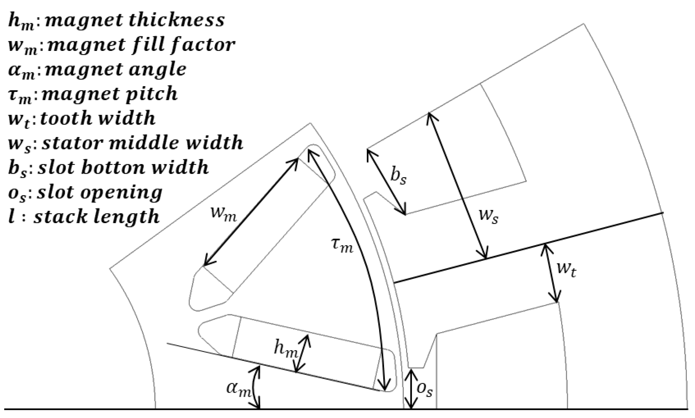
In this section, key information is provided for the optimization of a traction IPM machine. This baseline machine was initially designed for a micro EV application. Figure 2 shows the geometric design parameters of a 12 kW, 12-slot, 10-pole baseline IPM machine. Seven geometric parameters—magnet thickness h m , magnet fill factor w m , magnet angle α m , magnet pitch τ m , tooth width ratio ζ , slot opening ratio ξ , and stack length l —have been selected as the design variables for the optimization problem, as these parameters have a significant impact on average torque, torque ripple, active material cost, and total machine mass. The slot opening ratio ξ and tooth width ratio ζ can be expressed as:
ξ = o s b s
ζ = w t w s
where b s is the slot bottom width, o s is the slot opening, w t is the tooth width, and   w s is the stator middle width, as shown in Figure 2.
Table 1 shows the design requirements, machine parameters, and design variables.

4. Surrogate Model Construction

4.1. Surrogate Modeling Techniques

4.1.1. Kriging

Kriging is an interpolation method proposed by South African mining engineer Danie G. Krige, originally used to predict the distribution of minerals [28]. In recent decades, Kriging has gained widespread use as a tool for approximating the relationship between the inputs and outputs of a function.
Figure 3 presents an overlay plot with the Kriging predictions, the original function, and the observed data points. The observed data points are depicted as red points, and the Kriging model is constructed using these observations to calculate the prediction and confidence interval. The x-axis represents the input data value, and the y-axis represents the corresponding output value. The gray area indicates the normally distributed confidence intervals.
The basic assumption of the Kriging technique is that the predicted deterministic response, y ^ ( x ) , consists of a global model and local variations, which can be mathematically expressed as [29]:
y ^ ( x ) = p ( x ) + Z ( x )
where p(x) is the global model function, Z ( x ) is a random process based on a normal Gaussian distribution. The localized variations are accounted for by Z ( x ) , and its covariance can be expressed as [30]:
C o v [ Z ( x i ) , Z ( x j ) ] = σ 2 R ( x i , x j )
where R ( x i , x j ) is the spatial correlation function between the data points, and σ 2 is the variance. The correlation function R ( x i , x j ) is given as:
R ( x i , x j ) = exp ( l = 1 d θ l | x i x j | 2 )
where θ l is known as the hyperparameter. Using (1)–(3), the Kriging-predicted response can be expressed as follows [31]:
y ^ ( x ) = β + r T ( x ) R 1 ( y I β )
where r(x) is the correlation vector, I is the unit vector whose diagonal elements are filled with 1’s, and β is the vector of unknown regression coefficients.
The prediction capability of a Kriging model can vary significantly depending on the values of its hyperparameter. Kriging has been extensively studied and used by researchers in various fields of engineering due to its high prediction accuracy and versatility in handling various data configurations [32,33].

4.1.2. Artificial Neural Network

ANNs are computational systems inspired by the structure and function of neurons in the human brain [34]. The most common form of ANNs is a multilayer feedforward architecture comprising an input layer, one or more hidden layers, and an output layer, as illustrated in Figure 4. In this figure, the red, blue, and green nodes represent the input, hidden, and output layers, respectively.
The computational nodes of the hidden layers consist of neurons that form the basis for constructing ANNs. A normalized output is produced by each neuron by multiplying the activation function by the sum of the weighted inputs and the bias. This may be expressed as [35]:
y = δ ( j = 1 n w j x j + b )
where x j is the j-th input signal, w j is the j-th weight of the neuron, b is the bias, δ is the activation function, and y is the output signal.
The optimal weight matrix for each neuron can be determined using the backpropagation method, which feeds the error between the predicted and actual values back into the neural network. The prediction accuracy of ANNs is greatly influenced by various hyperparameters, including the number of neurons and hidden layers, the types of activation functions, and the learning rates. These parameters play a key role in determining the performance of ANNs.

4.1.3. Support Vector Regression

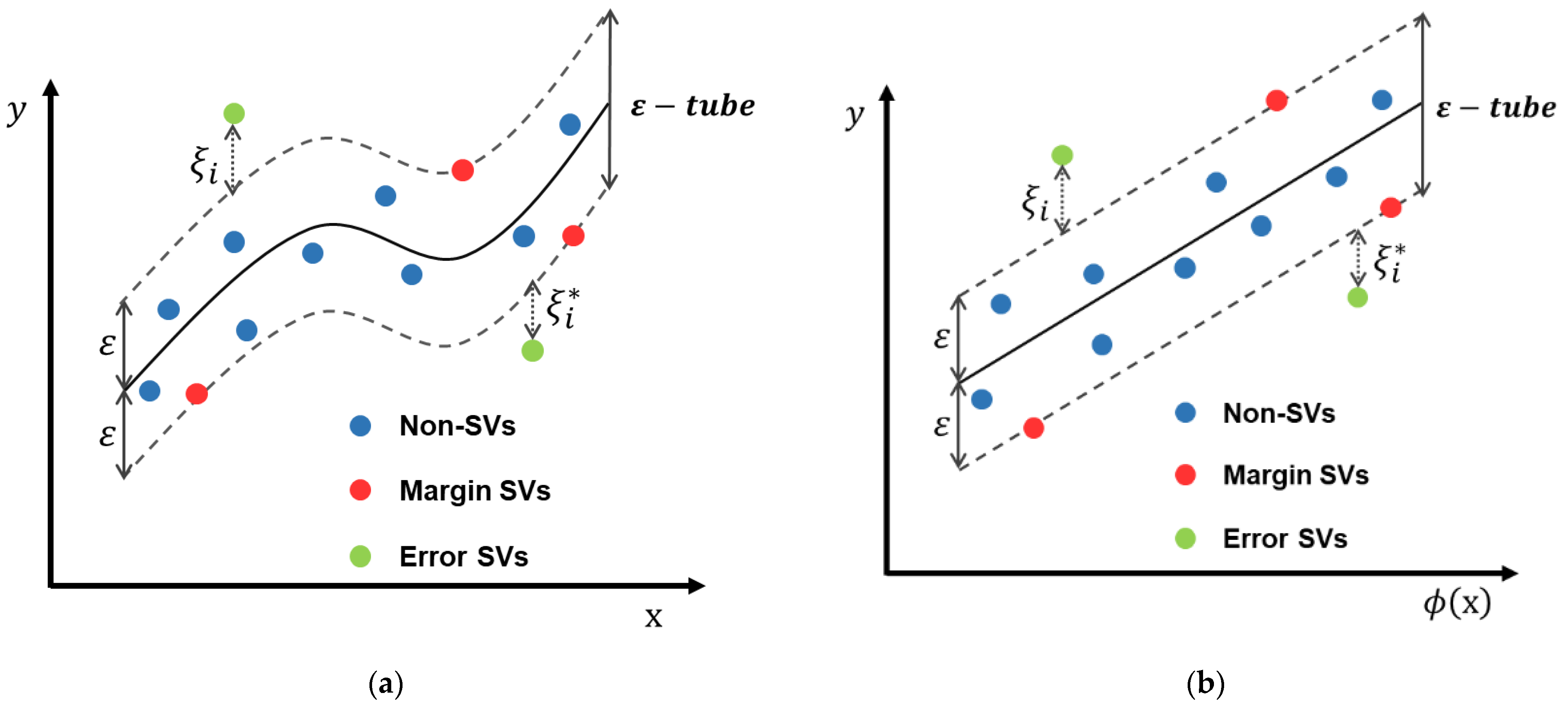
SVR is a variant of a support vector machine (SVM), a supervised learning algorithm commonly used for prediction in machine learning. SVR is a generalization of SVM that can be applied to regression problems. The underlying principle of SVR is to create a hyperplane (i.e., decision boundary) that separates the data into two classes based on the maximum margin theory. As illustrated in Figure 5, SVR maps the original dataset to a higher-dimensional feature space, treating it as a high-dimensional linear regression problem.
The linear separating line (solid black) in Figure 5b is a hyperplane which can be written as [36]:
f ( x ) = w · x + b
where w is the weight vector, b is the bias, and <wx> is the dot product of w and x.
According to [37], it is possible to calculate the optimal values of w and b as an optimization problem as follows:
M i n i m i z e :   1 2 w T w + C i = 1 n ( ξ i + ξ i * )
S u b j e c t   t o :   y i w T ϕ ( x i ) b ε + ξ i
w T ϕ ( x i ) + b y i ε + ξ i * ,
ξ i 0 ,     ξ i * 0
where n is the number of samples, C is the regularization hyperparameter which is greater than zero, ξ i and ξ i * are the slack variables, ϕ is the kernel function, ε is the deviation margin from the separating line, x i is ith sample which is mapped to a higher dimensional space by the kernel function.
The main principle of SVR is to use the kernel function to map the dataset x i into a higher-dimensional space through nonlinear mapping between the input space and feature space. A penalty is imposed on data points that lie outside the ε margin. The slack variables, ξ i and ξ i * , are introduced to relax the constraint by allowing for the inclusion of data points outside the margin when no further solution is available.

4.2. Hyperparameters of Surrogate Model

Hyperparameters are variables that are specified by the user prior to the start of SM training. These hyperparameters are not part of the SM itself, but they significantly affect the accuracy of model predictions. In contrast, model parameters are values that are automatically learned from a given dataset. Table 2 summarizes the hyperparameters and parameters used in the three different SM techniques discussed earlier.
There are several common methods for identifying a set of near-optimal hyperparameters, including rules of thumb, using legacy values, and trial-and-error methods such as grid search and random search. Grid search [38] and random search [39] can be suitable for experienced users, but grid search has the disadvantage of requiring a large number of evaluations when exploring high-dimensional spaces. Random search can be an alternative to such cases, but it does not always guarantee an optimal solution. In this study, we employ Bayesian optimization to efficiently and automatically adjust the hyperparameters.
Bayesian optimization (BO) is derived from Bayes’ theorem [40] and is a widely used framework for globally optimizing an unknown objective function. BO tests the values of the HPs by incorporating pre-calculated information in searching for optimal values. The BO process consists of two parts: an SM that provides a stochastic estimate of the unknown function and an acquisition function that generates the next candidate HP values to be tested based on the results of the SM [41]. This process is repeated until the convergence criteria are met. Gaussian process, tree-structured Parzen estimator, and random forest regression are among the most commonly used SM techniques. Expected improvement and probability of improvement are popular types of acquisition functions [42].
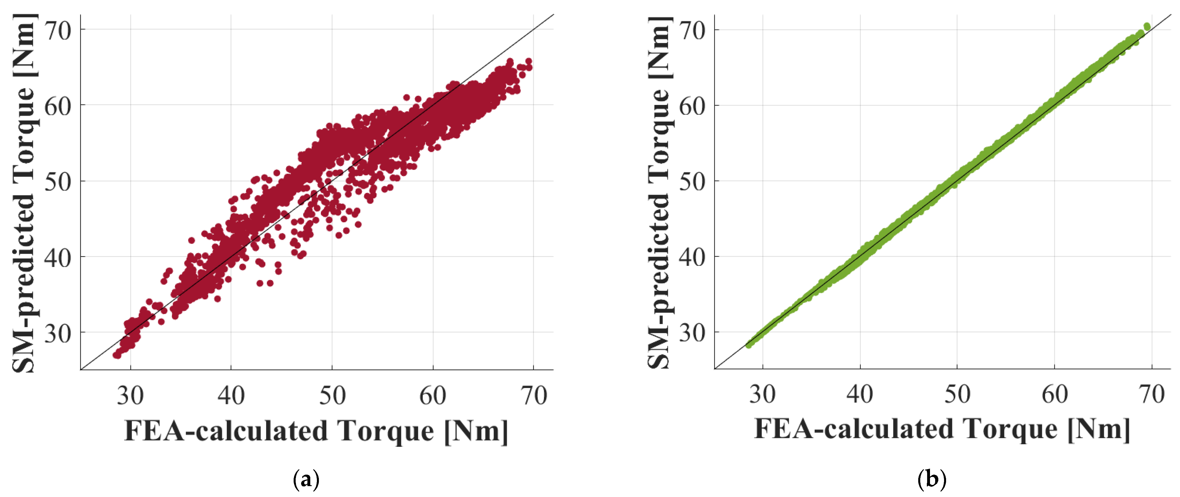
Figure 6 compares the average torque of an electric machine design obtained using ANN-based SM and FEA. The number of FEA calculation results used in the SM training was 300. As shown in the figure, the model performance improved significantly after the hyperparameters were tuned using Bayesian optimization.

4.3. Transition from FEA-Based to Surrogate-Based Optimization

Once the accuracy of the SM reaches a certain level, a stopping criterion is necessary to determine when to terminate the iterative training process. There are several commonly used stopping criteria that have been adopted by many researchers, including time spent, number of iterations, rate of change of the variable of interest, and accuracy target [33]. In this paper, we use a combination of three stopping criteria—accuracy target, rate of change, and number of iterations—as convergence criteria to prevent the optimization algorithm from continuing unnecessarily.
Of the three criteria, the accuracy target is chosen as the first convergence criterion. To this end, RMSE, one of the standard methods for evaluating the prediction error of a model, is used as a key metric comparing the results from FEA and SM. The mathematical expression of the RMSE can be written as:
  RMSE = 1 n i = 1 n ( y i y ^ i )
where y i is the ith data calculated using FEA and y ^ i is the predicted value by SM.
Convergence occurs when the RMSE value is less than 0.5% of the average of the total accumulated FEA calculation results. This can be expressed as follows:
  RMSE     1 n i = 1 n y i × 0.5 %
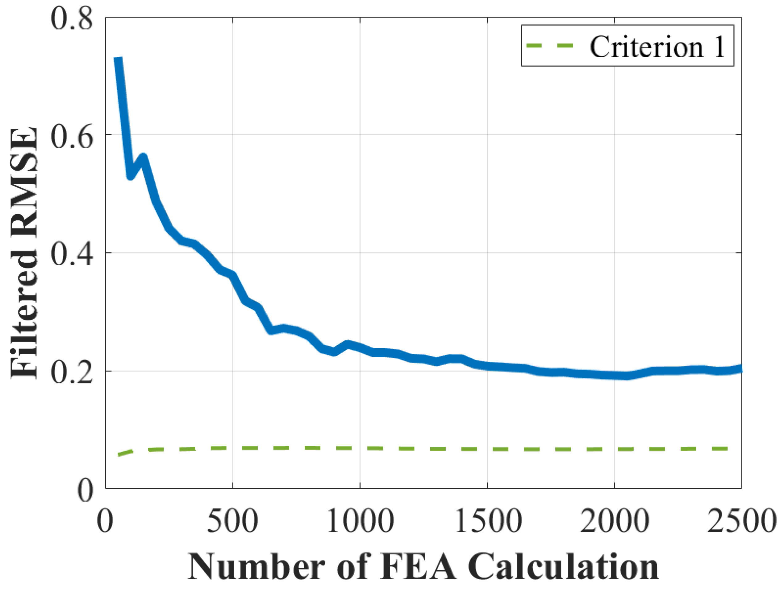
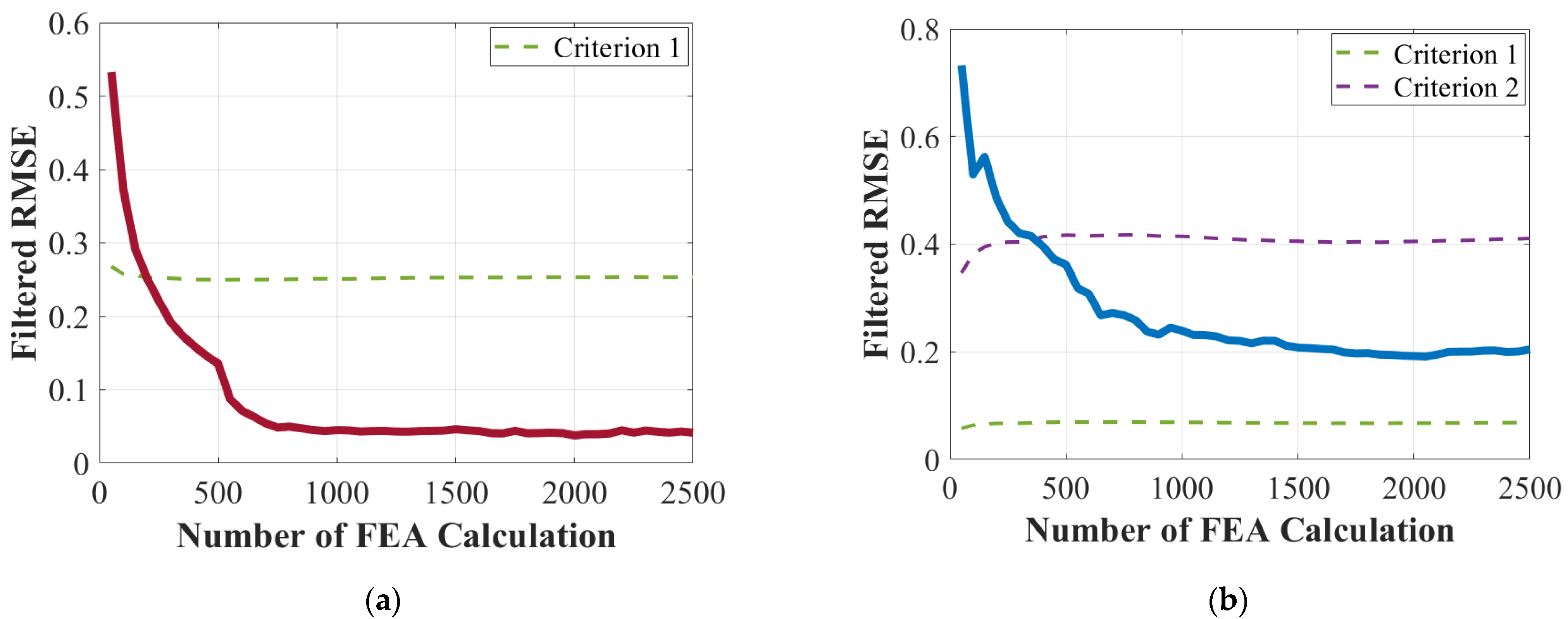
This first convergence criterion can be evaluated with a relatively small amount of FEA results if the input–output relationship exhibits a linear response. In the cases studied in this paper, it was found that generating 50 to 200 FEA samples was sufficient to train the SMs for most objective functions. However, not all SMs will necessarily satisfy this convergence criterion. For example, some SMs or objective functions may exhibit more nonlinear characteristics, requiring a larger number of calculations to converge. As shown in Figure 7, the torque ripple data requires more FEA samples to reach the RMSE criterion explained in (12) than the average torque and material cost. The figure illustrates the RMSE of the SM as a function of the number of FEA calculations used to construct the SM.
The fact that the RMSE value in Figure 7 does not change much as the number of calculations increases suggests that convergence is imminent, and therefore, there is no need to add more FEA calculations and retrain the SMs. To address this issue, we introduce a second convergence condition that uses the rate of change in the RMSE value as a metric. A moving average (MA) filter [43] is applied to the last 10 data points to smooth out random spikes in raw data caused by the stochastic nature of the SM construction process. Since the change in prediction accuracy is significant at the beginning of SM construction, the MA filter is applied after the first 10 calculations.
The final stopping criterion is the maximum number of iterations allowed, which is set to 50 (2500 FEA calculations) in this study. It has been reported [44] that this number of iterations is sufficient for the optimization process to converge. The three stopping criteria described above are summarized as follows:
  • Criterion 1: Stop if the RMSE is equal to or less than 0.5%;
  • Criterion 2: Stop if the sign of the rate of change changes from negative to positive and RMSE is equal to or less than 3% after 10 iterations (500 FEA calculations);
  • Criterion 3: Stop if the number of calculations is greater than 50 iterations (2500 FEA calculations).
If none of the above criteria are satisfied, the SM building process will be repeated by adding the calculated FEA results to the SM training dataset. Figure 8a and 8b show two examples of satisfying the first and second stopping criteria, respectively. Figure 8a shows a case that requires only 200 FEA results to converge, while Figure 8b shows that 700 FEA results are needed to meet the second criterion when the first criterion is not satisfied. Ultimately, the optimization process depicted in Figure 1 transitions from an FEA-based to an SM-based approach when the stopping criterion is met.

4.4. Data Clustering Technique for Pareto Front Verification

After completing the surrogate-assisted optimization process using the NSGA-II algorithm, a set of Pareto non-dominated designs and a Pareto front are generated in the design space. Since the generated Pareto front is based on approximations using SMs, an FE-based verification process is required. However, typical Pareto fronts consist of a large number of design samples, and the verification step can be time-consuming. One way to reduce computational time is to perform verification using a representative group of the design samples. To improve the efficiency of the verification process, we use the k-means clustering technique [45] to group the entire Pareto front samples into a specified number of clusters. The k-means clustering algorithm finds cluster centroids through an iterative process that minimizes the sum of squared distances between each data point and the nearest cluster centroids [46]. The sum of squared distance can be defined as follows [47]:
Sum   of   the   squared   distance   = i = 1 n { min k = 1 , 2 , , K d ( x i , c k ) } 2
where x is the location of individual data points, c is the nearest cluster center, d is the Euclidean distance between two points, and K is the number of partitions.
An example of clustered Pareto front samples is shown in the next Section. The use of the k-means algorithm reduces the total number of Pareto front samples that need to be verified by approx—95.6%. The computational time saved increases as the numbers of generations and populations grow.

5. Optimization Results

5.1. Performance Comparison between SMs

The predictive performance of the SMs is evaluated and compared with respect to the four design objective functions: average torque, torque ripple, total machine mass, and active material cost (AMC). The AMC is calculated as a function of the cost and mass of the active material and can be written as follows:
AMC = p p m · m p m + p c u · m c u + p f e · m f e
where p p m is the PM’s cost per kilogram, p c u is the copper’s cost per kilogram, and p f e is the iron cost per kilogram, all expressed in (USD/kg). The specific values for each active material used in the traction machine are 118 USD/kg, 9.44 USD/kg, and 2.36 USD/kg for PM, copper, and iron, respectively. The m stands for the mass of each active material.
Figure 9a–d shows the trend of the filtered RMSE values of three SMs, Kriging, ANN, and SVR, for each objective function according to the number of FEA calculations. Figure 9a shows that the total machine mass was well predicted using a relatively small number of FEA calculations, regardless of the SM type. This is because the change in total mass is not very sensitive to most design variables, except stack length. The predicted results of all SMs meet the first stopping criterion with only 50 FEA calculation results. In contrast, most design variables, particularly rotor variables, show higher sensitivity to AMC and average torque, so more FEA calculations are required to complete SM training and meet the stopping criterion. As shown in Figure 9b,c, it took no more than 350 FEA calculations to train the SMs to predict AMC and average torque with adequate accuracy.
It is well known that torque ripple is very sensitive to small changes in design variables and can be as high as 20% to 100% under key operating conditions if not carefully designed [48,49]. Therefore, it is very challenging for the torque ripple responses to satisfy the first stopping criterion with a reasonable number of FEA calculations, and the convergence condition needs to be relaxed by lowering the accuracy target or using another stopping criterion. Figure 10 shows the change in the filtered RMSE values according to the number of FEA calculations for the three SMs with torque ripple as the objective function. It can be seen in Figure 10 that Kriging and ANN satisfy the second stopping criterion with 700 and 950 FEA calculations, respectively. On the other hand, the SVR prediction results did not satisfy either the first or second criterion, and the iterative SM building process was stopped when the maximum number of FEA calculations (i.e., 2500) was reached.
Table 3 shows the number of FEA calculations required for the SMs to satisfy the stopping criteria for each objective function. Of the three SMs tested, it can be seen that Kriging produced a high-performance approximation model using a minimal amount of FEA data for all objective functions. On the other hand, it was confirmed that SVR requires a relatively large number of FEA calculations to converge, and the variability of prediction results is very high. As mentioned earlier, approximating torque ripple requires the largest number of FEA calculations to converge due to its highly nonlinear input–output relationship.

5.2. Comparative Analysis: FEA-Based vs. SM-Based Optimization Process

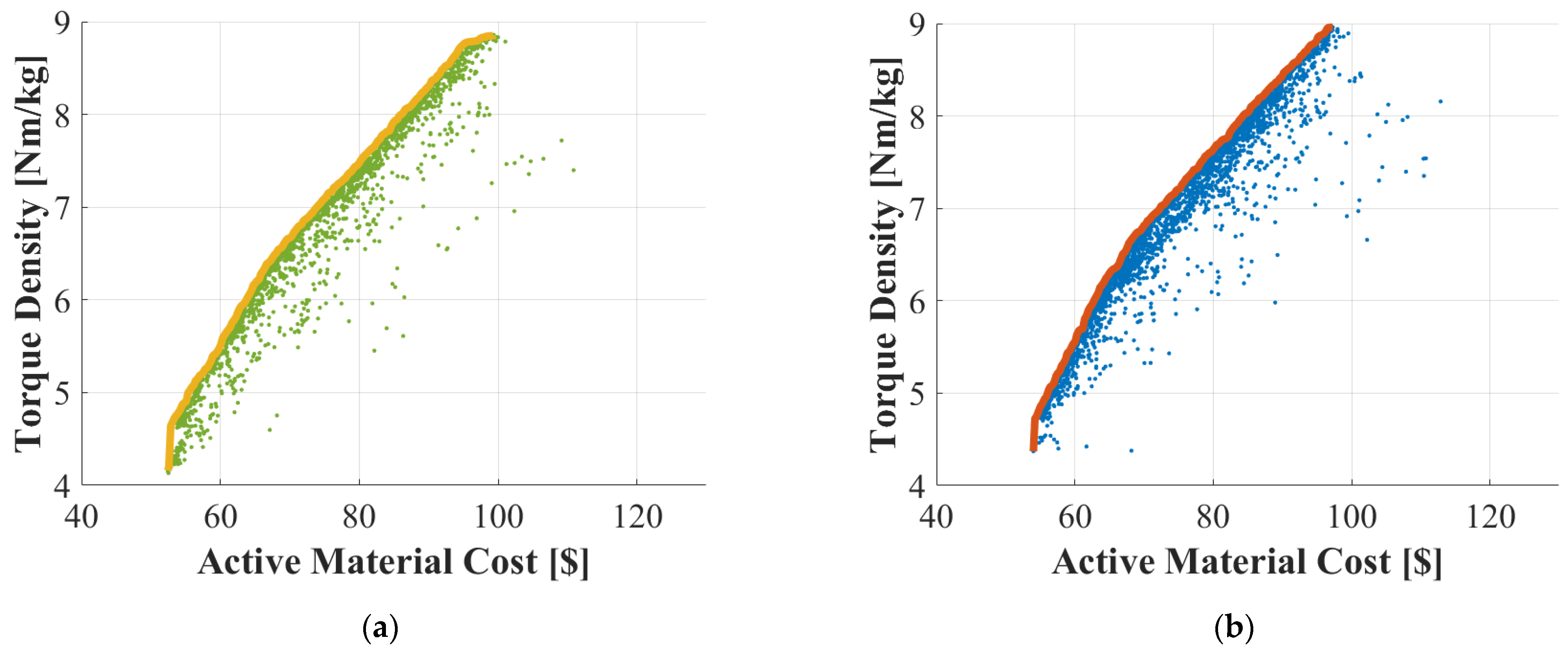
In this section, the results of design optimization based on FEA and those using surrogated-assisted optimization are compared. The same design variables and conditions as in Table 1, as well as the objective functions of AMC in dollars and torque density in Nm/kg, are considered. The defined prices of each active material are 118 USD/kg for magnet, 9.4 USD/kg for copper, and 2.4 USD/kg for iron. For the optimization problem, 100 generations with a population size of 50 per generation, a crossover probability of 0.9, and a mutation probability of 0.05 were chosen.
Based on the results in Section 5.1, Kriging was identified as the most accurate surrogate modeling technique among the three methods and was used to construct the SMs. Figure 11a,b show the distributions of individual non-dominated designs and the Pareto fronts calculated during each FEA-based and SM-based optimization process, respectively, confirming that there is excellent agreement between the two results. The Kriging-based SMs for the two objective functions were trained using 250 FEA data samples per SM, and their hyperparameters were tuned using Bayesian optimization, as described in Section 4.2.
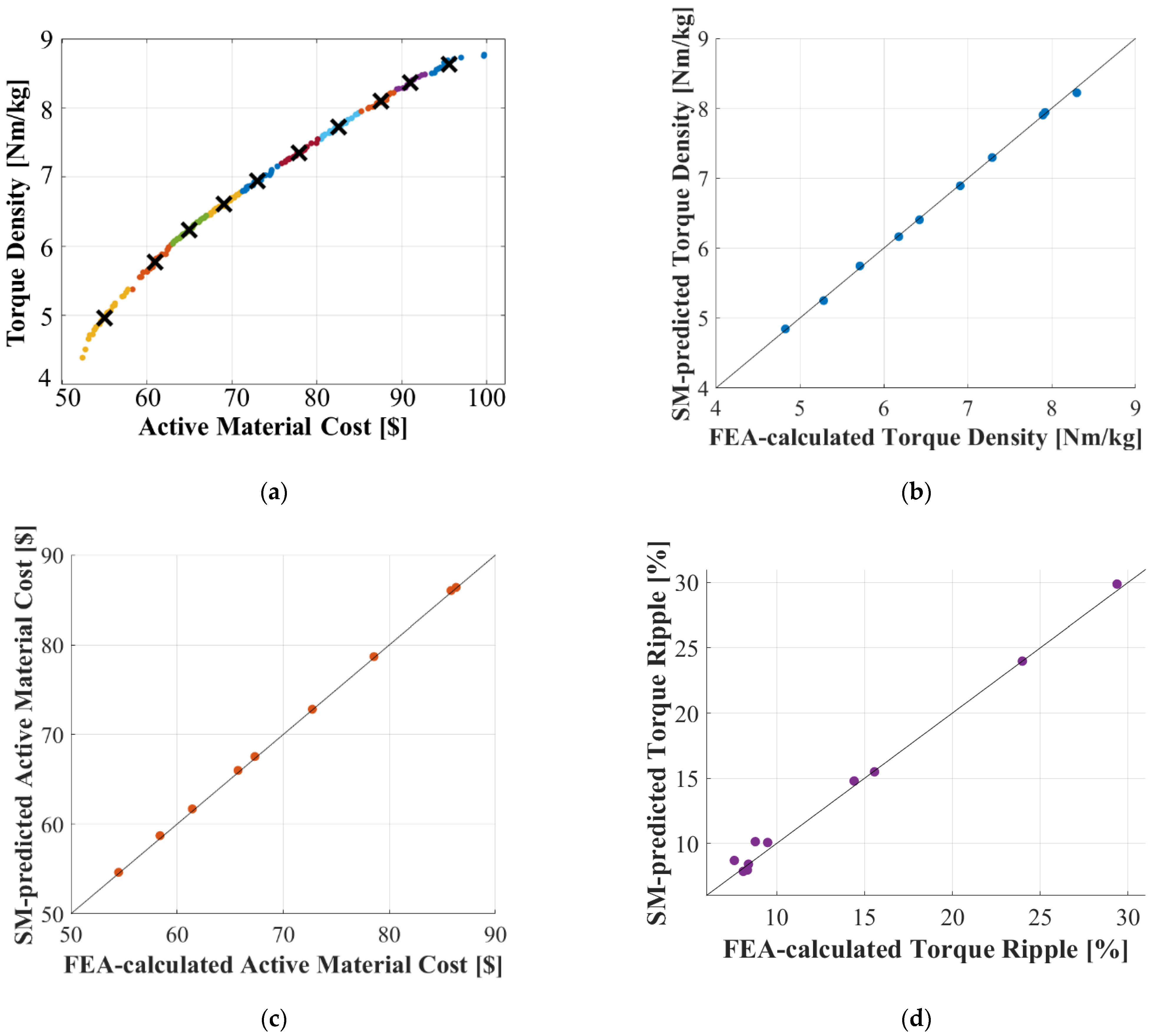
After conducting the SM-based optimization process, the final results (see Figure 11) were validated using FEA to ensure the accuracy of the SM predictions. In this specific optimization problem, which involved two objective functions, we select 10 representative samples from the Pareto front to verify as the set of optimal solutions lies on this Pareto front. Figure 12a shows the representative samples (marked with X), which were identified using the k-means clustering technique and extracted from a total of 227 data points on the Pareto front, reducing the number of data points requiring verification by 95.6%. Figure 12b–d presents the error between FEA results and SM predictions for each of the 10 representative samples for three different objective functions, torque density, active material cost, and torque ripple. The average errors for the AMC and torque density objectives were USD 0.196 and 0.0243 Nm/kg, respectively, both of which are less than 1%. The torque ripple error increases at lower ripple values, but the absolute value of the error is still within 1.35%.
It is worth mentioning that, in cases where the number of objective functions is greater than two, the optimal solution to an optimization problem is likely to be found among the Pareto non-dominant designs rather than on the Pareto front when considering the associated engineering trade-offs. While this is beyond the scope of this paper, there have been several studies addressing this issue [12,16]. Overall, the proposed design process has achieved a significant reduction in calculation time, with a total calculation time reduction of approx. 93% compared to the conventional FEA-based approach while maintaining an accuracy error within 1%.
Finally, the specifications of the computer used in this study are shown in Table 4.

6. Conclusions and Future Works

In this paper, we present a surrogate-assisted design optimization process using an NSGA-II algorithm for electric machine applications. Our simulation results demonstrate that the proposed approach outperforms the conventional method, which relies on FEA and empirical tuning. In addition, we provide a thorough explanation of the various components that make up the proposed optimization process. The major contributions of this paper are summarized as follows:
  • Comparison of three different surrogate modeling techniques, Kriging, ANN, and SVR;
  • Introduction of an automated HP tuning process through Bayesian optimization;
  • Development of robust three-step stopping criteria that determine the transition from FEA-based to SM-based optimization;
  • Detailed analysis of the approximation accuracy of various SMs for four different objective functions considering the number of FEA results used for SM training and HP tuning effect;
  • Reduction of calculation time for verification of the Pareto front predicted by SM using the k-means clustering technique;
  • Computational time savings of more than 90% with no loss of accuracy compared to FEA-based optimization.
Also, we found that the samples distributed in the two-dimensional objective space using the proposed approach closely agreed with the results obtained using the conventional FEA-based approach. In addition, we observed a significant reduction in overall computation time of approx. 93% when compared to the traditional FEA-based method while maintaining an accuracy error of less than 1%.
The proposed process has the potential to be applied to optimize various types of electric machines for a range of applications. It has also been developed as a guideline for electric machine designers who may have limited experience with the nuances of constructing and tuning SMs and metaheuristic optimization algorithms.
In future work, we plan to extend the proposed process to more complex optimization problems with a larger number of design variables and more challenging design requirements. While this study focused on the design of electric machines with a single operating point, it is necessary to consider the entire drive cycle for the design of traction machines for EV applications. Therefore, further research is required to adapt the proposed process to consider multiple operating points simultaneously. Finally, we will investigate the potential for further improvements in computation time through the use of advanced techniques such as reduced-order modeling and adaptive sampling.

Author Contributions

Methodology, software, formal analysis, validation, data curation, writing—original draft preparation, M.C.; conceptualization, methodology, formal analysis, writing—original draft preparation, review and editing, supervision, G.C.; conceptualization, writing—review, G.B.; conceptualization, writing—review, E.M. All authors have read and agreed to the published version of the manuscript.

Funding

This work was supported in part by the NRF (National Research Foundation) grant funded by the Korean government (MSIT: Ministry of Science and ICT) (grant number: 2021R1F1A1048754); and in part by the NRF of Korea grant funded by the Korean government (MSIT) (grant number: 2022K1A3A1A18080373).

Data Availability Statement

Not applicable.

Conflicts of Interest

The authors declare no conflict of interest.

References

  1. Perujo, A.; Ciuffo, B. The Introduction of Electric Vehicles in the Private Fleet: Potential Impact on the Electric Supply System and on the Environment. A Case Study for the Province of Milan, Italy. Energy Policy 2010, 38, 4549–4561. [Google Scholar] [CrossRef]
  2. Choi, G.; Bramerdorfer, G. Comprehensive Design and Analysis of an Interior Permanent Magnet Synchronous Machine for Light-Duty Passenger EVs. IEEE Access 2022, 10, 819–831. [Google Scholar] [CrossRef]
  3. Johansson, T.B.; van Dessel, M.; Belmans, R.; Geysen, W. Technique for Finding the Optimum Geometry of Electrostatic Micromotors. IEEE Trans. Ind. Appl. 1994, 30, 912–919. [Google Scholar] [CrossRef]
  4. Bianchi, N.; Bolognani, S. Design Optimisation of Electric Motors by Genetic Algorithms. IEE Proc. Electr. Power Appl. 1998, 145, 475–483. [Google Scholar] [CrossRef]
  5. Uler, G.F.; Mohammed, O.A.; Chang-Seop, K. Design optimization of electrical machines using genetic algorithms. IEEE Trans. Magn. 1995, 31, 2008–2011. [Google Scholar] [CrossRef]
  6. Gao, J.; Sun, H.; He, L. Optimization design of Switched Reluctance Motor based on Particle Swarm Optimization. In Proceedings of the 2011 International Conference on Electrical Machines and Systems (ICEMS), Beijing, China, 20–23 August 2011; pp. 1–5. [Google Scholar]
  7. Mutluer, M.; Bilgin, O. Design Optimization of PMSM by Particle Swarm Optimization and Genetic Algorithm. In Proceedings of the INISTA 2012—International Symposium on Innovations in Intelligent Systems and Applications, Trabzon, Turkey, 2–4 July 2012. [Google Scholar]
  8. Duan, Y.; Harley, R.G.; Habetler, T.G. Comparison of Particle Swarm Optimization and Genetic Algorithm in the design of permanent magnet motors. In Proceedings of the 2009 IEEE 6th International Power Electronics and Motion Control Conference, Wuhan, China, 17–20 May 2009; pp. 822–825. [Google Scholar]
  9. Kennedy, J.; Eberhart, R. Particle swarm optimization. In Proceedings of the ICNN’95—International Conference on Neural Networks, Perth, Australia, 27 November–1 December 1995; pp. 1942–1948. [Google Scholar]
  10. Murata, T.; Ishibuchi, H.; Sanchis, J.; Blasco, X. MOGA: Multi-objective genetic algorithms. In Proceedings of the IEEE International Conference on Evolutionary Computation, Perth, WA, Australia, 29 November–1 December 1995; IEEE: Piscataway, NJ, USA, 1995; Volume 1, pp. 289–294. [Google Scholar]
  11. Zhang, Q.; Li, H. MOEA/D: A multiobjective evolutionary algorithm based on decomposition. IEEE Trans. Evol. Comput. 2007, 11, 712–731. [Google Scholar] [CrossRef]
  12. Li, Y.; Lei, G.; Bramerdorfer, G.; Peng, S.; Sun, X.; Zhu, J. Machine Learning for Design Optimization of Electromagnetic Devices: Recent Developments and Future Directions. Appl. Sci. 2021, 11, 1627. [Google Scholar] [CrossRef]
  13. Song, J.; Dong, F.; Zhao, J.; Wang, H.; He, Z.; Wang, L. An Efficient Multiobjective Design Optimization Method for a PMSLM Based on an Extreme Learning Machine. IEEE Trans. Ind. Electron. 2019, 66, 1001–1011. [Google Scholar] [CrossRef]
  14. You, Y.-M. Multi-Objective Optimal Design of Permanent Magnet Synchronous Motor for Electric Vehicle Based on Deep Learning. Appl. Sci. 2020, 10, 482. [Google Scholar] [CrossRef] [Green Version]
  15. Kim, S.; You, Y. Optimization of a Permanent Magnet Synchronous Motor for e-Mobility Using Metamodels. Appl. Sci. 2022, 12, 1625. [Google Scholar] [CrossRef]
  16. Zăvoianu, A.-C.; Bramerdorfer, G.; Lughofer, E.; Silber, S.; Amrhein, W.; Klement, E.P. Hybridization of multi-objective evolutionary algorithms and artificial neural networks for optimizing the performance of electrical drives. Eng. Appl. Artif. Intell. 2013, 26, 1781–1794. [Google Scholar] [CrossRef]
  17. Deb, K.; Pratap, A.; Agarwal, S.; Meyarivan, T. A fast and elitist multiobjective genetic algorithm: Nsga-II. IEEE Trans. Evol. Comput. 2002, 6, 182–197. [Google Scholar] [CrossRef] [Green Version]
  18. Jeyakumar, D.N.; Venkatesh, P.; Lee, K.Y. Application of multi objective evolutionary programming to combined economic emission dispatch problem. In Proceedings of the 2007 International Joint Conference on Neural Networks, Orlando, FL, USA, 12–17 August 2007; pp. 1162–1167. [Google Scholar]
  19. El-Nemr, M.; Afifi, M.; Rezk, H.; Ibrahim, M. Finite Element Based Overall Optimization of Switched Reluctance Motor Using Multi-Objective Genetic Algorithm (NSGA-II). Mathematics 2021, 9, 576. [Google Scholar] [CrossRef]
  20. Jo, S.-T.; Kim, W.-H.; Lee, Y.-K.; Kim, Y.-J.; Choi, J.-Y. Multi-Objective Optimal Design of SPMSM for Electric Compressor Using Analytical Method and NSGA-II Algorithm. Energies 2022, 15, 7510. [Google Scholar] [CrossRef]
  21. Pereira, L.A.; Haffner, S.; Nicol, G.; Dias, T.F. Multiobjective optimization of five-phase induction machines based on NSGA-II. IEEE Trans. Ind. Electron. 2017, 64, 9844–9853. [Google Scholar] [CrossRef]
  22. Chekroun, S.; Abdelhadi, B.; Benoudjit, A. A New Approach Design Optimizer of Induction Motor Using Particle Swarm Algorithm. AMSE J. 2014, 87, 89–108. [Google Scholar]
  23. Shayanfar, H.; Gharehchopogh, F.S. Farmland fertility: A new metaheuristic algorithm for solving continuous optimization problems. Appl. Soft Comput. 2018, 71, 728–746. [Google Scholar] [CrossRef]
  24. Abdollahzadeh, B.; Gharehchopogh, F.S.; Khodadadi, N.; Mirjalili, S. Mountain Gazelle Optimizer: A New Nature-Inspired Metaheuristic Algorithm for Global Optimization Problems. Adv. Eng. Softw. 2022, 174, 103282. [Google Scholar] [CrossRef]
  25. Abdollahzadeh, B.; Soleimanian Gharehchopogh, F.; Mirjalili, S. Artificial Gorilla Troops Optimizer: A New Nature-Inspired Metaheuristic Algorithm for Global Optimization Problems. Int. J. Intell. Syst. 2021, 36, 5887–5958. [Google Scholar] [CrossRef]
  26. Gharehchopogh, F.S. Quantum-inspired metaheuristic algorithms: Comprehensive survey and classification. Artif. Intell. Rev. 2022, 1, 1–65. [Google Scholar] [CrossRef]
  27. Im, S.Y.; Lee, S.G.; Kim, D.M.; Xu, G.; Shin, S.Y.; Lim, M.S. Kriging SM-Based Design of an Ultra-High-Speed Surface-Mounted Permanent-Magnet Synchronous Motor Considering Stator Iron Loss and Rotor Eddy Current Loss. IEEE Trans. Magn. 2022, 58, 8101405. [Google Scholar] [CrossRef]
  28. Cressie, N. The origins of kriging. Math. Geol. 1990, 22, 239–252. [Google Scholar] [CrossRef]
  29. Zhao, L.; Wang, P.; Song, B.; Wang, X.; Dong, H. An efficient kriging modeling method for high-dimensional design problems based on maximal information coefficient. Struct. Multidiscip. Optim. 2019, 61, 39–57. [Google Scholar] [CrossRef]
  30. Toal, D.J.J.; Bressloff, N.W.; Keane, A.J. Kriging hyperparameter tuning strategies. AIAA J. 2008, 46, 1240–1252. [Google Scholar] [CrossRef]
  31. Sacks, J.; Welch, W.J.; Mitchell, T.J.; Wynn, H.P. Design and Analysis of Computer Experiments. Statist. Sci. 1989, 4, 409–435. [Google Scholar] [CrossRef]
  32. Van, J.; Guibal, D. Beyond ordinary kriging—An overview of non-linear estimation. In Beyond Ordinary Kriging: Non-Linear Geostatistical Methods in Practice; The Geostatistical Association of Australasia: Perth, Australia, 1998; pp. 6–25. [Google Scholar]
  33. Fuhg, J.N.; Fau, A.; Nackenhorst, U. State-of-the-art and Comparative Review of Adaptive Sampling Methods for Kriging. In Archives of Computational Methods in Engineering; Leibniz Universität Hannover, Université Paris-Saclay: Hannover, Germany; Paris, France, 2021; Volume 28. [Google Scholar]
  34. McCulloch, W.; Pitts, W. A Logical Calculus of Ideas Immanent in Nervous Activity. Bull. Math. Bio. Phys. 1943, 5, 115–133. [Google Scholar] [CrossRef]
  35. Balázs, C.C. Approximation with Artificial Neural Networks. Master’s Thesis, Eötvös Loránd University, Budapest, Hungary, 2001. [Google Scholar]
  36. Alex, J.S.; Schölkopf, B. A tutorial on support vector regression. Statist. Comput. 2014, 14, 199–222. [Google Scholar]
  37. Drucker, H.; Burges, C.J.C.; Kaufman, L.; Smola, A.; Vapnik, V. Support vector regression machines. Adv. Neural Inf. Process. Syst. 1997, 9, 155–161. [Google Scholar]
  38. Zahedi, L.; Mohammadi, F.G.; Rezapour, S.; Ohland, M.W.; Amini, M.H. Search Algorithms for Automated Hyper-Parameter Tuning. arXiv 2021, arXiv:2104.14677. [Google Scholar]
  39. Bergstra, J.; Bengio, Y. Random Search for Hyper-parameter Optimization. J. Mach. Learn. Res. 2012, 13, 281–305. [Google Scholar]
  40. Swinburne, R. Bayes’ Theorem. Rev. Philos. Fr. 2004, 194, 2825–2830. [Google Scholar]
  41. Wu, J.; Hao, X.C.; Xiong, Z.L.; Lei, H. Hyperparameter Optimization for Machine Learning Models Based on Bayesian Optimization. J. Electron. Sci. Technol. 2019, 17, 26–40. [Google Scholar]
  42. Cho, H.; Kim, Y.; Lee, E.; Choi, D.; Lee, Y.; Rhee, W. Basic Enhancement Strategies When Using Bayesian Optimization for Hyperparameter Tuning of Deep Neural Networks. IEEE Access 2020, 8, 52588–52608. [Google Scholar] [CrossRef]
  43. Zeaiter, M.; Rutledge, D. Preprocessing Methods. In Comprehensive Chemometrics: Chemical and Biochemical Data Analysis; Brown, S.D., Tauler, R., Walczak, B., Eds.; Elsevier: Amsterdam, The Netherlands, 2009; pp. 121–231. ISBN 978-0-444-52701-1. [Google Scholar]
  44. Querin, O.M.; Victoria, M.; Alonso, C.; Ansola, R.; Martí, P. Topology Design Methods for Structural Optimization; Elsevier: Amsterdam, The Netherlands, 2017; ISBN 9780081009161. [Google Scholar]
  45. Bejarano, L.A.; Espitia, H.E.; Montenegro, C.E. Clustering Analysis for the Pareto Optimal Front in Multi-Objective Optimization. Computation 2022, 10, 37. [Google Scholar] [CrossRef]
  46. Lloyd, S.P. Least Squares Quantization in PCM. IEEE Trans. Inf. Theory 1982, 28, 129–137. [Google Scholar] [CrossRef] [Green Version]
  47. Redmond, S.J.; Heneghan, C. A method for initialising the K-means clustering algorithm using kd-trees. Pattern Recognit. Lett. 2007, 28, 965–973. [Google Scholar] [CrossRef]
  48. Han, S.H.; Jahns, T.M.; Soong, W.L.; Guven, M.K.; Illindala, M.S. Torque Ripple Reduction in Interior Permanent Magnet Synchronous Machines Using Stators With Odd Number of Slots Per Pole Pair. IEEE Trans. Energy Convers. 2010, 25, 118–127. [Google Scholar] [CrossRef]
  49. Sanada, M.; Hiramoto, K.; Morimoto, S.; Takeda, Y. Torque Ripple Improvement for Synchronous Reluctance Motor Using an Asymmetric Flux Barrier Arrangement. IEEE Trans. Ind. Appl. 2004, 40, 1076–1082. [Google Scholar] [CrossRef]
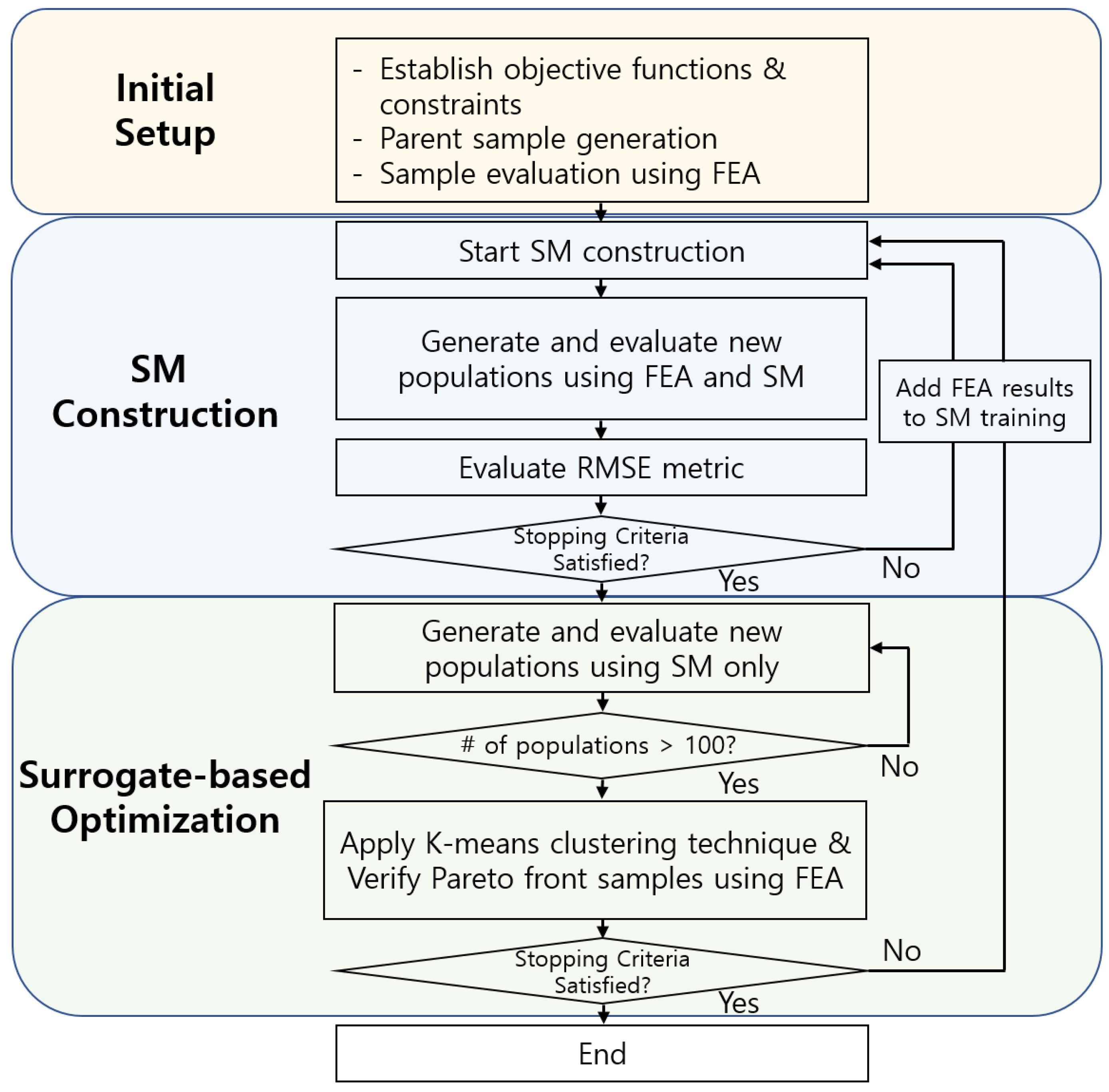
Figure 1. Flowchart of surrogate-assisted design optimization process for electric machines.
Energies 16 00392 g001
Figure 2. Machine cross-section and key design variables.
Energies 16 00392 g002
Figure 3. Kriging prediction (solid black line) using the observed data (red dots) with the original function (red dashed line) and 95% confidence interval (gray area).
Energies 16 00392 g003
Figure 4. ANN structure with multilayer feedforward architecture.
Energies 16 00392 g004
Figure 5. A structure of one-dimensional support vector regression. (a) Before mapping the dataset into a higher-dimensional feature space. (b) After mapping the dataset into a higher-dimensional feature space.
Energies 16 00392 g005
Figure 6. An example showing the impact of Bayesian optimization-based hyperparameter tuning. (a) SM vs. FEA without hyperparameter tuning. (b) SM vs. FEA with hyperparameter tuning.
Energies 16 00392 g006
Figure 7. An example of Criterion 1 not being met when the accuracy target is set too low.
Energies 16 00392 g007
Figure 8. Two examples of completing the iterative SM building process (point of convergence marked with gray circle). (a) Case 1: Criterion 1 is met. (b) Case 2: Criterion 2 is met.
Energies 16 00392 g008
Figure 9. Filtered RMSE trends according to the number of FEA calculations. (a) Total machine mass (kg). (b) Active material cost ($). (c) Average torque (Nm). (d) Torque ripple (%). Grey circles indicate convergence points.
Energies 16 00392 g009
Figure 10. Torque ripple prediction accuracy using three SMs according to the number of FEA calculations. Grey circles indicate convergence points.
Energies 16 00392 g010
Figure 11. 2D objective space projections of the Pareto non-dominated designs after running the design optimization process using NSGA-II algorithm. (a) FEA-based results. (b) SM-based results.
Energies 16 00392 g011
Figure 12. Optimization result evaluation: (a) 2D objective space projection of the Pareto front (colored dots) and extracted representative samples (black X), (b) Torque density prediction of each representative sample point, (c) Active material cost prediction of each representative sample point, (d) Torque ripple prediction of each representative sample point.
Energies 16 00392 g012
Table 1. Key performance requirements, constant parameters, and design variables.
ParameterValue
Peak Current Density15 Arms/mm2
Slot/Pole12/10
Peak Power/Peak Torque15 kW/70 Nm
Peak Current150 Arms
Series Turns17 Turns
Rotor Diameter110 mm
Airgap Length0.75 mm
Magnet Remanence1.1 T at 100 °C
Magnet GradeNMX-36EH (Hitachi)
Lamination Grade35JN300 (JFE)
Design Variables and Their Range h m = [ 4.2 ,   5.4 ]   mm
w m = [ 0.7 ,   0.91 ]
α m = [ 17.5 ,   32.5 ] °
τ m = [ 0.85 ,   0.99 ]
ξ = [ 0.4 ,   0.6 ]
ζ = [ 0.4 ,   0.6 ]
l = [ 50 ,   65 ]   mm
Table 2. Key performance requirements, constant parameters, and design variables.
Type of SMParameter (s)Hyperparameter (s)
KrigingCorrelation matrix, vector θ l
ANNWeight, biasNumber of hidden layers, neurons, and activation function
SVRSupport vectorRegularization hyperparameter, kernel function
Table 3. The number of FEA calculations required to satisfy the stopping criteria.
Objective FunctionKrigingANNSVR
Total Mass505050
Active Material Cost5050100
Average Torque50200350
Torque Ripple7009502500
Table 4. A Summary of Computer Specifications.
Processing UnitAMD Ryzen 9 5900X 12-Core
Processor, 3.70 GHz
Operating SystemWindows 11 Pro (64-bit)
Random Access Memory32 GB DDR4
Data Storage TypeSSD SATA
Graphic CardNVIDIA GeForce GTX 1650
Disclaimer/Publisher’s Note: The statements, opinions and data contained in all publications are solely those of the individual author(s) and contributor(s) and not of MDPI and/or the editor(s). MDPI and/or the editor(s) disclaim responsibility for any injury to people or property resulting from any ideas, methods, instructions or products referred to in the content.