Abstract
As a kind of clean energy, the exploration and development of coalbed methane (CBM) are of great importance and significance. In this paper, the CBM reservoir parameters of a working area in Western Guizhou Province, China, were predicted by using 3D seismic exploration technology, and the sweet-spot area was evaluated based on the prediction results. In terms of data interpretation, while the traditional technology is extended to the study of CBM, new technologies and methods suitable for CBM were also actively explored, especially in the quantitative prediction methods of parameters such as coal seam thickness, CBM content, coal body structure, in situ stress, etc., and a three-highs quantitative prediction technology of CBM sweet spots characterized by high precision, high resolution, and high coincidence was explored, which is based on logging evaluation and petrophysics. In addition, in the comprehensive evaluation of multiparameter sweet spots, the multiparameter weighted step-by-step evaluation method based on inversion was innovatively proposed, which made the prediction of CBM sweet spots more focused, effective, and practical, and the distribution law of sweet spots was more consistent with the geological law, providing enough basis for subsequent well location deployment. Based on this method, the C409 coal seam was selected as the sweet spot.
1. Introduction
China first proposed the strategic goals of a carbon peak in 2030 and a carbon neutral 2060 in 2020 [1]. Therefore, the utilization of renewable energy, sustainable energy, and clean energy is of great importance and significance. Due to the intermittence of photovoltaic, hydropower, and wind energy, the utilization of unconventional natural gas such as CBM and shale gas is also a meaningful way to realize the low-carbon strategy. CBM is a kind of unconventional natural gas with methane as the main component in the coal seam, which is mainly absorbed on the surface of the coal matrix and partially free in pore cracks or dissolved in the coal seam water. It has the characteristics of high calorific value, low emission, and low pollution.
Guizhou Province is a large province of coal resources, as well as CBM, in the south of China, which is very rich in coal resources and contains a large amount of CBM resources for exploitation and utilization. The coal-bearing area of the province is about 77,500 km2, accounting for 44% of the total area of the region. The Upper Permian Longtan Formation is the most important coal-bearing formation in the Western Guizhou area of Guizhou Province. It is widely distributed, well developed, and rich in fossils. The Upper Permian consists of clastic rocks intercalated with carbonate rocks and coal seams, and is rich in coal and CBM resources. According to the Evaluation of CBM Resource Potential in Guizhou Province, the CBM geological resources of the Upper Permian strata in Guizhou Province are 3056.19 billion m3, and the average abundance of CBM resources is 112 million m3/km2. The recoverable geological resources of CBM are 1379.13 billion m3, accounting for 45.31% of the total resources. The gas content of 500 m deep coal seams in the Longtan Formation in Western Guizhou is generally between 8.0 and 25.0 m3/t, with an average of about 12.0–15.0 m3/t.
Seismic exploration technology [2,3,4] is often used to find out the spatial distribution, structural morphology, fracture development, and other characteristics of coal reservoirs, and to analyze and interpret the fracture distribution and in situ stress characteristics of coal reservoirs. Seismic exploration is a geophysical exploration method to infer the nature and form of underground rock strata by observing and analyzing the propagation law of seismic waves generated by artificial earthquakes based on the difference in elasticity and density of the underground medium. Seismic exploration is the most important and effective method to solve oil and gas exploration problems in geophysical exploration [5]. It is an important means of exploration of petroleum and natural gas resources before drilling, and has been widely used in coalfield and engineering geological exploration, regional geological research, and crustal research [6,7,8].
Gong [9] proposed a 3D seismic exploration signal acquisition method in a high-density coal mine area, and it has been well verified. In situ stress is the critical factor to determine the shape, orientation, and extension direction of generated fractures, so the prediction of in situ stress is the basis of CBM reservoir exploitation. Ma et al. [10], considering both the effect of vertical cracks in HTI media and the effect of horizontal bedding in VTI media, derived the expression of in situ stress in orthotropic (OA) media based on orthotropic media theory, and realized the seismic prediction of in situ stress by using azimuth-prestack seismic data. Tiğrek et al. [11] first used reflection coefficient inversion to obtain dynamic parameters, then used the relationship between dynamic and static parameters to obtain the parameters of the geomechanical model, and finally obtained the distribution of in situ stress based on the geomechanical model. Kumar et al. [12] developed a method for evaluating reservoir porosity using poststack seismic data for both excellent and poor impedance porosity correlations. Ali et al. [13] applied poststack seismic inversion techniques to estimate reservoir properties (such as acoustic impedance and porosity) in a gas-bearing reservoir in the Sawan area of the Indus Basin in southern Pakistan. Negm et al. [14], based on poststack inversion and the multiattribute lambda-mu-Rho (LMR) method, predicted the Dutch North Sea gas content. In order to achieve accurate inversion of poststack acoustic impedance, Morozov et al. [15] proposed a synthetic logging curve construction method that clearly and accurately satisfies the convolution equation, the time-depth constraint of seismic data, and the low-frequency model of logging or seismic/geological interpretation background. Based on deep-learning methods, according to Meng et al. [16], compared with traditional geophysical inversion, deep-learning inversion can give inversion results with higher resolution.
In this study, a work area in Western Guizhou Province, China, was chosen as the study case, and 3D seismic exploration was conducted. A progressive reservoir prediction solution consisting of four methods (poststack impedance inversion, poststack geostatistical inversion, simultaneous prestack inversion test, and prestack geostatistical inversion) was selected to interpret the result of 3D seismic exploration. Coal seam thickness, CBM content, coal body structure, and in situ stress were well interpreted. In addition, in the comprehensive evaluation of multiparameter sweet spots, the multiparameter weighted step-by-step evaluation method based on inversion was innovatively proposed, which made the prediction of the CBM sweet spot more focused, effective, and practical, and the distribution law of sweet spots was more consistent with the geological law, providing enough basis for subsequent well location deployment.
2. Geological Conditions of the Work Area
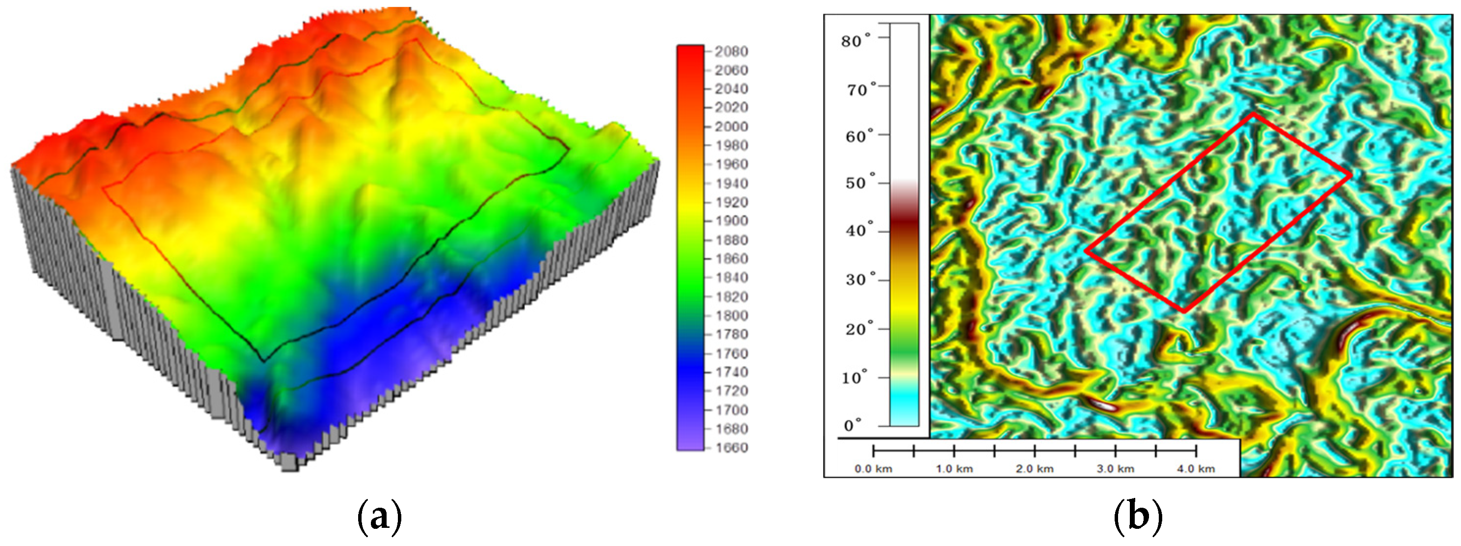
The work area is located in the Wumeng Mountain area in Western Guizhou Province of the Yunnan–Guizhou Plateau. The landform is mainly mountainous and hilly. The overall elevation trend of the work area is high in the west and low in the east, with an altitude between 1600 and 2100 m and a local height difference of more than 300 m (Figure 1a). The surface slope of the work area is relatively slow, mostly at 15–30° and partially above 40° (Figure 1b).
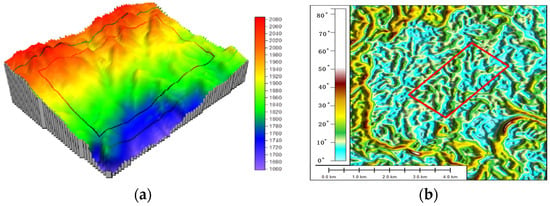
Figure 1.
Elevation map (a) and surface slope plan (b) of work area.
The Middle Permian Qixia Maokou Formation, the Lower Triassic Yongningzhen Formation, and the middle-upper member of the Middle Triassic Guanling Formation in the region are all soluble rocks, with many fissured caves and strong water content, which are essential aquifers. The Emeishan Basalt Formation, the Longtan Formation of the Upper Permian, and the Feixianguan Formation of the Lower Triassic are mostly argillaceous siltstone and silty mudstone with weak water content and permeability, which are the relative water-resisting layer between the above aquifers, as shown in Table 1 [17].

Table 1.
Hydrogeological characteristics of the regional water-resisting layer.
The overlying aquifer of coal measures strata is limestone karst water of the Yongningzhen Formation, and the underlying aquifer is limestone karst water of the Maokou–Qixia Formation (Figure 2), which has large water storage space and strong water content, but it is far away from the coal seam and is blocked by the relative water-resisting layer of the Feixianguan Formation and the Emeishan basalt, which is poor in coal seam replenishment and beneficial to CBM preservation.

Figure 2.
Diagram of position relation between coal-bearing formation and aquifer (Note: RWRL: relative water-resisting layer, T1f3: Member 3 of Feiguan Formation; T1f4: Member 4 of Feiguan Formation; P3c: Changxing Formation, Upper Permian; P3l: Longtan Formation, Upper Permian; P2m: Maokou Formation, Middle Permian).
The prominent outcrops are Triassic (T) and Permian (P), with a small amount of Carboniferous (C) and Quaternary (Q). The lithology of outcrops is mainly carbonate rock (limestone, dolomite), and clay rock, basaltic lava, chert limestone, shale, and quaternary clay are also widely distributed. The carbonate rock area is characterized by poor water content, karst caves and fractures, serious energy loss, fast attenuation of effective waves, and poor excitation and receiving conditions. The coal measure strata are well developed in this area, which has the function of shielding energy and a low signal-to-noise ratio.
According to the previous seismic data, the structure of the study area is relatively complex, generally characterized by comb-like folds, well-developed normal faults, and a wide and gentle anticline and narrow syncline, and minable coal seams are often distributed along the anticline axis or wing parts, with great differences between east and west.
There are some structures in the Liupanshui coalfield, such as the Gemudi syncline, the Weishui syncline, the Okawabe syncline, the Tudiya syncline, and the Yangmeishu syncline. The syncline is the main coal-bearing structural unit in the Liupanshui coalfield, but faults can often destroy the continuity of the coal seams. Faults are well developed in the study area. In the south of the syncline, the faults strike northeast, and most of them are low-angle normal faults. In the north of the syncline, the fault strike is mainly NW, and most of them are high-angle reverse faults. The Weining–Ziyun structural deformation area where the Dahebian syncline is located underwent intense folding and fracture during the Yanshan period, and under the control of basement fracture, an NW-trending deformation area was formed, which made the central–northern axis of the Dahebian syncline NW-trending, and at the same time, various faults in the north NW-trending were formed. In the south of the syncline, the structural line changed from the NW direction to the NE direction due to the interference of the turbine-like structure of the child thrust. The tectonic movement in the study area runs through the whole process of coalbed methane generation, migration, and diffusion. This area’s fault is mostly cemented by argillaceous and calcite veins, with suitable sealing properties. The difference in CBM content between the upper and lower coal seams of the fault and water inflow per unit of pumping test indicates that the fault in this area is relatively closed, which is beneficial to the preservation of CBM.
The exposed strata in the study area mainly include the Upper Permian Emeishan Basalt Formation (P2β), the Longtan Formation (P2l) and Wangjiazhai Formation (P2wj), the Lower Triassic Feixianguan Formation (T1f), the Yongningzhen Formation (T1yn), the Middle Permian Guanling Formation (T2g), and Quaternary (Q). Among them, the Permian and Triassic strata are the most widely distributed [18]. The Liangshan Formation of the Middle Permian, the Emeishan Basalt Formation of the Upper Permian, the Longtan Formation, the Changxing Formation, and the Huobachong Formation of the Upper Triassic are the main coal-bearing strata, among which the Longtan Formation of the Upper Permian has the best coal-bearing property [19].
Two geological sections of the northwest wing and southeast wing of the Dahebian syncline were selected for analysis. The strata in the north of the west wing of the syncline are mainly composed of Quaternary (Q), the Feixianguan Formation (T1f), the Longtan Formation (P2l), the Wangjiazhai Formation (P2wj), and the Emeishan Basalt Formation (P2β), but the Yongningzhen Formation (T1yn) and the Guanling Formation (T2g) are missing. The thickness of the Feiguan Formation (T1f) gradually became thinner from southwest to northeast until it was pointed out, reaching the 2303 borehole in the north of the syncline. The Wangjiazhai Formation (P2wj) was completely denuded, and the Longtan Formation (P2l) was partially denuded, with only the remaining Longtan Formation (P2l) and Emeishan Basalt Formation (P2β) lying in the lower part of Quaternary (Q). In the BB’ section, the strata mainly include Quaternary (Q), the Yongningzhen Formation (T1yn), the Feixianguan Formation (T1f), the Longtan Formation (P2l), the Wangjiazhai Formation (P2wj), and the Emeishan Basalt Formation (P2β), but the Guanling Formation (T2g) is missing, and the strata are exposed completely in the west wing of the syncline.
In the past, there were strong reflection interfaces in the shallow, middle, and deep layers of seismic profiles in the study area. There were many sets of strong reflection interfaces in many coal seams developed in the Permian, and the overlying coal seams can be tracked continuously. Because the upper coal seams have a strong shielding effect on reflected signals, the reflected information of underlying coal seams is weak, and the continuity of reflected waves is slightly poor. The target strata of this study are mainly coal measures strata of the Longtan Formation (P2l) of the Upper Permian, C605-C504 strata (the upper coal seams), and C409-C406 strata (the lower coal seams).
In summary, due to the multistage tectonic movement in the study area, strip segmentation is formed, and the reflection information of the fracture zone is weak. The shallow coal seam in the study area has a strong shielding effect on the deep strata, resulting in energy scattering.
The construction mode of 3D seismic exploration was centralized acquisition after all wells were drilled, and the tasks of drilling and acquisition were assigned by dividing blocks according to the terrain. In the acquisition stage, the whole work area was paved with 5074 detection points, and then the acquisition was started. The SmartSolo 10 Hz node instrument was used to receive the data, and the borehole gun self-excitation system was used to shoot. In the field acquisition process, information such as the position and parameters of each shot file and each array sheet was recorded. After the acquisition was completed, the data were merged and cut with the support of SmartSolo technology. Then, technicians checked the shot information records, various shift reports, original shot sets, and superimposed profiles, and performed quality rating, which fundamentally guaranteed the quality of all original data. The drilling shot points in the work area are in accordance with the predesigned shot points, as shown in Figure 3.
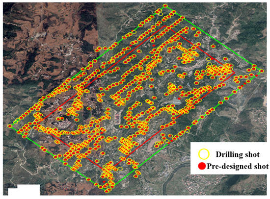
Figure 3.
Drilling shot and predesigned shot map.
3. Methods
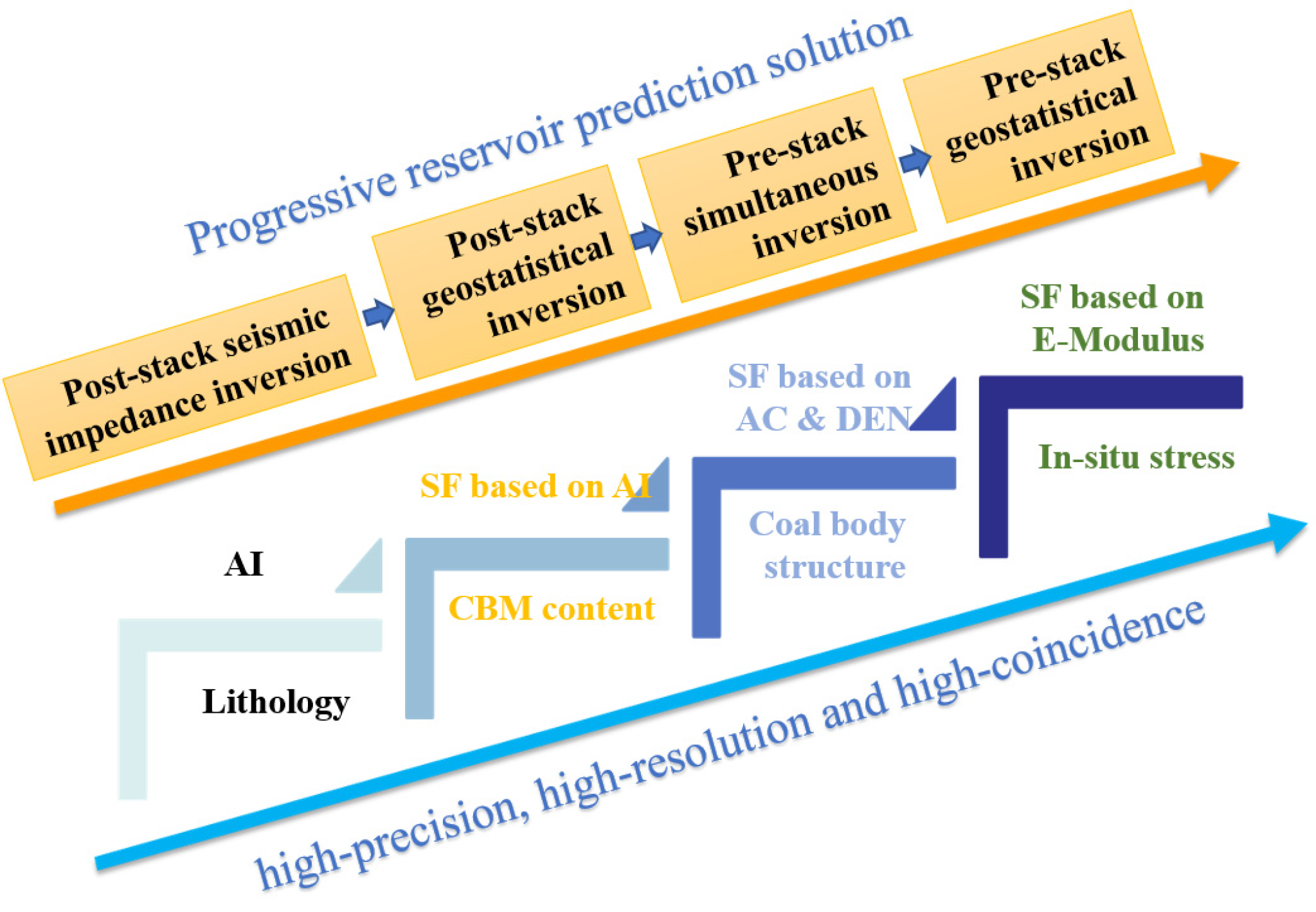
Through fine petrophysical analysis, the sensitive parameters of lithology identification, CBM content identification, coal body structure identification, and in situ stress identification are defined, and the elastic parameters obtained by inversion are P-wave impedance (or P-wave velocity), S-wave impedance (or S-wave velocity), density, etc. This means that the simple poststack impedance cannot meet the demand. At the same time, combined with the geological characteristics of the thin coal seam in this area, deterministic inversion cannot meet the resolution requirements, so geostatistical inversion should be introduced. To perform a high-precision and high-resolution inversion well, it is necessary to test the parameters of the various methods step by step according to the idea of increasing predictable parameters and improving prediction accuracy step by step, so as to understand the prediction ability of seismic data and logging data. Therefore, this study designed a progressive reservoir prediction solution, as shown in Figure 4.
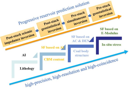
Figure 4.
Diagram of the progressive reservoir prediction solution.
According to the above reservoir prediction ideas, the Jason geological research platform of CGG company was selected to carry out work in this study. The Jason platform has a relatively complete prestack and poststack, deterministic and statistical inversion methods, and a high market share among similar commercial software, so it can meet the needs of this study. At each stage of modeling, the well velocity and synthetic seismic records should be referred to in order to determine the trend of velocity change. At each stage of velocity analysis, whether CRP gathers are straight or not should be taken as the quality control standard. The specific process is as follows: high-quality prestack depth migration imaging depends on the high-precision subsurface macroscopic layer velocity model. The velocity-depth model has two elements: the macroscopic layer velocity interface and the layer velocity values of the corresponding layers. An accurate velocity model must describe the distribution of the underground velocity field within a tectonic framework. Therefore, the method based on stratum has become the most commonly used method in modeling. At present, the prestack depth migration velocity is calculated by iteration.
We conducted a lithology sensitivity analysis, gas content sensitivity analysis, and coal structure sensitivity analysis. The lithology sensitivity analysis shows that DTC and DTS basically have no discrimination ability for sand and mudstone, but they have good discrimination for coal seams. As for Vp/Vs, there is basically no discrimination ability for sandstone and mudstone. Although coal seams can reflect the general trend of low Vp/Vs, they overlap seriously. The gas content sensitivity analysis is shown in Section 4.2. The coal structure sensitivity analysis shows that RT is the most sensitive to coal structure and can be used to determine the classification of coal structure. However, it has been verified by drilling in this area that the logging curves of the primary structure coal are characterized by low CAL value, high Rt value, and low Gr value, but the RT logging curves of fractured coal and structural coal overlap seriously, so it is difficult to effectively distinguish the coal structure in this area by using RT curves. The logging curves of coal seams in this area have the characteristics of high resistance, high acoustic wave, large neutron, low density, low natural gamma, and hole diameter enlargement.
3.1. Poststack Seismic Impedance Inversion Test
Although the conventional poststack seismic impedance inversion [20,21] can only obtain P-wave impedance with a single elastic parameter, it is widely used because of its relatively simple operation, low requirements for basic data, sound wave and/or density logging curves, and poststack seismic data.
Under the condition that P-wave impedance has a certain ability to identify lithology, it can achieve better results. According to the previous petrophysical analysis, the P-wave impedance of the Dahebian syncline coal seam and the non-coal seam is obviously different. Therefore, it is necessary to test the poststack seismic impedance inversion, implement the correlation of well-seismic calibration, and investigate the stability of the wavelet. All these aspects provide basic quality control and input data for subsequent inversion methods, and also clarify the basic prediction ability of seismic and logging data. Therefore, although parameter prediction does not depend on the results of poststack seismic impedance inversion, testing it is an important workflow.
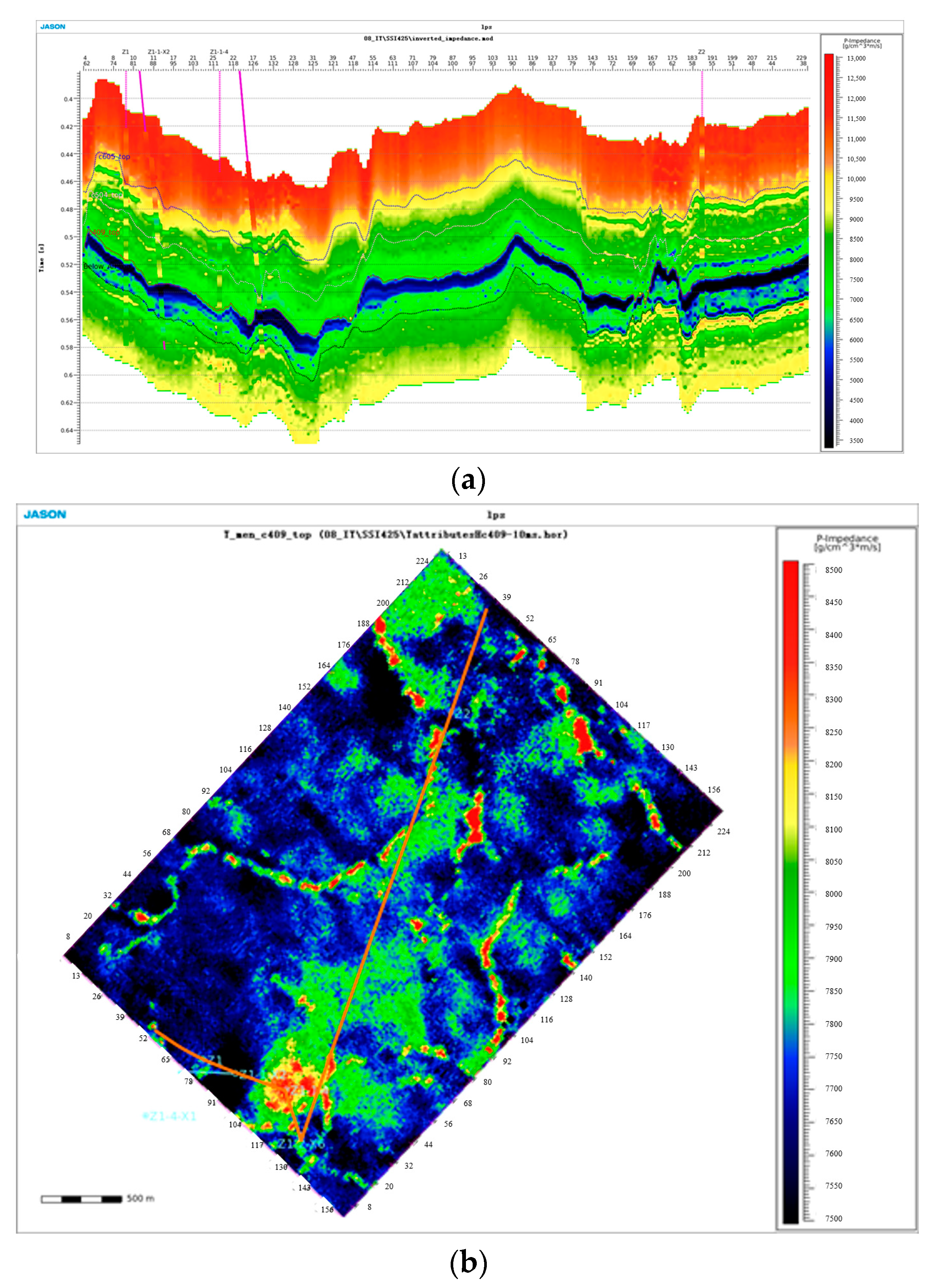
As shown in Figure 5a, the cross-section of the poststack seismic impedance inversion well connection in this work area shows that the coal seam can be well identified, but there is basically no ability to distinguish sand–mudstone, which is consistent with the petrophysical analysis conclusion. As shown in Figure 5b, from the P-wave impedance plan of the thickest C409 coal seam in this area, poststack seismic inversion can predict the change characteristics of coal seam thickness to a certain extent, which shows that this poststack seismic inversion test achieved the expected effect.

Figure 5.
Poststack seismic impedance inversion section (a) and plan (b) of Dahebian syncline.
3.2. Poststack Geostatistical Inversion Test
Statistical inversion [22] is an inversion method that combines stochastic simulation theory with seismic inversion. It consists of two parts, namely, the random simulation process and the process of optimizing the simulation results to match the seismic data. In practical work, geostatistical inversion first uses the deterministic inversion method to obtain the wave impedance body to know the approximate distribution of the reservoir, which can be used to determine the horizontal variogram function. Then, starting from the well points, cross-well wave impedance is generated by random simulation, and then wave impedance is converted into a reflection coefficient and convoluted with a wavelet obtained by the deterministic inversion method to generate a synthetic seismic trace. It is iterated repeatedly until the synthetic seismic trace matches the original seismic trace to a certain extent. This method effectively integrates geological, logging, and 3D seismic data. The inversion results are realized by several equal probability wave impedance data volumes, which are in line with the geostatistical characteristics of input data and constrained by geological models. It has the advantages of high vertical resolution of logging data and high lateral resolution of seismic data, and can be used for uncertainty evaluation.
Geostatistical inversion [23] has a high spatial resolution and is widely used in thin reservoir prediction. Depending on the characteristics of the geostatistical inversion method, it has a higher coincidence with the information on the well, and the reservoir characteristics and spatial distribution law are clearer.
Poststack geostatistical inversion [24] can directly obtain high-resolution elastic parameter P-wave acoustic impedance (AI), and other reservoir parameters can be simulated by cosimulation (on the premise that P-wave impedance has petrophysical sensitivity), and lithologic bodies can be directly obtained. As shown in Figure 6.
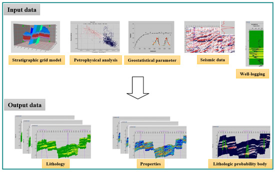
Figure 6.
Input–output diagram of poststack geostatistical inversion.
The accuracy of geological statistical inversion is greatly influenced by the geological framework model, longitudinal/transverse range, and spatial distribution trend of rocks. Therefore, it is necessary to test the vertical thickness and horizontal distribution of the geological bodies of coal seams and non-coal measures strata in this area by testing the poststack geostatistics inverse evolution difference function for parameter preparation for subsequent prestack geostatistical inversion.
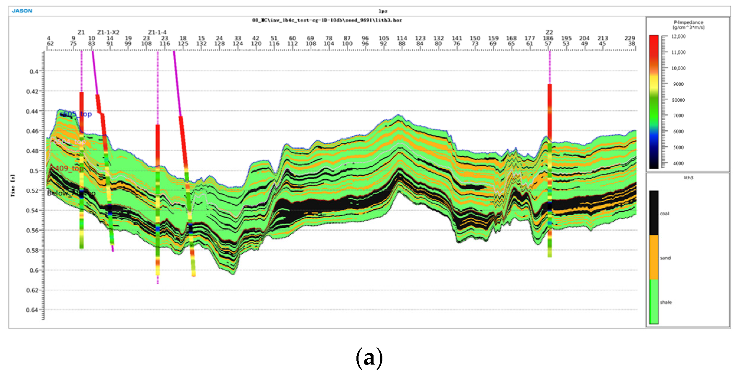
This poststack geostatistical inversion passed several rounds of parameter tests, and a good inversion result was obtained when the longitudinal range was 0.004 ms and the transverse field was 1000 m. From the profile of the well connection, as shown in Figure 7a,b, the vertical resolution of lithology realization and impedance realization is reasonable, and the horizontal distribution range of geological bodies is reasonable, with good accuracy. Therefore, this geostatistical inversion parameter test achieved the expected purpose.

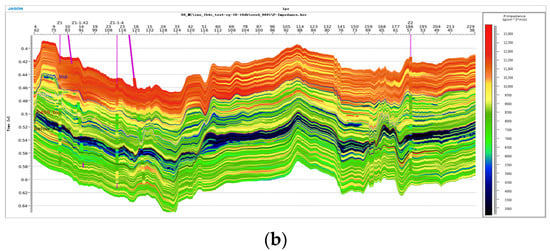
Figure 7.
Poststack geostatistical inversion lithology section and AI section: (a) lithology; (b) AI.
3.3. Prestack Simultaneous Inversion Test
Seismic waves carry a lot of characteristic information closely related to reservoir properties when they propagate in real earth media, and they have played a very important role in oil and gas exploration to use seismic data to predict reservoir lithology. Prestack seismic data contain abundant information about the variation of the seismic wave amplitude with offset. Through prestack seismic inversion, information such as P-wave velocity, S-wave velocity, and density can be obtained, and lithology-sensitive elastic parameters can be further calculated. Therefore, inversion of lithology-sensitive elastic parameters with prestack seismic data has become the primary technical means for lithologic reservoir prediction.
Simultaneous inversion of multiangle gathers (AVO/AVA-constrained sparse pulse simultaneous inversion) is based on the conventional constrained sparse pulse inversion technique applied to elastic inversion or wave impedance inversion. At the same time, according to the selected elastic parameter configuration, multiple seismic data volumes with different angles or offsets are simultaneously inverted to generate models such as P-wave impedance, S-wave impedance, and S-wave velocity ratio. The same convolution model is applied to each stack gathering data, and the reflection coefficient suitable for each stack gather data is determined by applying the Knott–Zoeppritz equation [25,26] or the Aki–Richards approximation equation [27]. At the same time, the inversion uses the same constrained sparse pulse inversion engine as the single-channel set data volume inversion, but there are extra data items in the objective function.
The elastic model generated by the AVO/AVA-constrained sparse pulse inversion algorithm has a wider bandwidth than the stack gathers of each input angle with the L1/L2 sparse criterion. The AVO/AVA-constrained sparse pulse inversion algorithm obtains the absolute elastic parameter model. The missing low-frequency components in the measured seismic data cannot be directly obtained by sparse pulse inversion, so it is necessary to establish a low-frequency trend model as the constraint condition of inversion. In the reflectivity domain, first, the unconstrained reflectivity inversion of the angular gather data is carried out. Through weighted superposition, the obtained reflection coefficient is converted into an elastic difference. The obtained elastic difference is further combined with the low-frequency model to form elastic parameters. For elastic parameters, fully constrained simultaneous inversion is carried out to improve the correlation between synthetic seismic records and input angle stack gather data. The combined frequency of the elastic difference and the low-frequency model is selected to ensure that more information can be obtained from the angular stack gather data, and the frequency spectrum gap can be avoided.
Because of the limited bandwidth of seismic data, the result of the sparse pulse is not unique. In order to make the elastic parameters obtained from sparse pulse inversion reasonable in geology and geophysics, it is necessary to minimize the introduction of random noise into the inversion results, and to add appropriate constraints for inversion.
Soft trend constraints include trend constraints, SVD stabilization, difference stabilization, and petrophysical equations.
The soft trend constraint conditions of the selected parameters (such as P-wave impedance, P-wave velocity ratio, and density) will make the result of sparse pulse inversion and the low-frequency trend model not change much. Band-pass filtering is carried out on the inverted model by combining frequencies. If the trends of the inverted elastic models are different, the soft trend constraint becomes a punishment condition to adjust the strength of the constraint condition, which can provide stable low-frequency results without significantly reducing the correlation between synthetic seismic records and seismic data.
SVD stabilization is a method to reduce the influence of noise at the expense of resolution. When the matrix is inverted, some small physical quantities in the matrix will cause instability. The SVD method first analyzes the matrix, and then adds the percentage of the maximum physical quantity to other physical quantities. The SVD constraint will make the result of density inversion more stable, but it greatly influences the velocity ratio of P-wave and S-wave.
Elastic parameters (P-wave impedance, P-wave velocity ratio, and density) for differential stabilization are chosen to make the weighted superposition process between unconstrained differential optimization and constrained elastic parameter optimization more stable.
In simultaneous inversion, unless the angle of stacked gather data changes greatly. If there are three or more substacked gathers, it is often difficult to obtain high-quality density. Therefore, applying Gardner’s and Mudrock’s [28] petrophysical equations as constraints can make the density result more stable. Gardner and Mudrock’s relative difference stabilization can make the weighted superposition process more stable, and it is also used to make the results of difference optimization and elastic parameter optimization more stable. Among them, the stabilization process of the soft Gardner constraint is realized by assuming the relationship between P-wave velocity and density, and the stabilization process of the soft Mudrock constraint is realized by assuming the relationship between P-wave velocity and S-wave velocity.
Relative stabilization is a compromise. Increasing the stabilization parameter will improve the stability of the inversion results, but will reduce the matching degree between synthetic seismic records and seismic data.
The soft space constraint is used to constrain the lateral divergence of inversion results in the lateral direction along the stratigraphic horizon. Random noise can be eliminated in the elastic parameter model, and the lateral continuity of the elastic model can be enhanced. Soft space constraints also help the models of P-wave impedance, S-wave impedance, and S-wave velocity ratio to be more stable and reduce the merging frequency.
In addition, in the case of applying soft space constraints, simultaneous inversion can operate on small pieces of 3D data volume, which makes it possible to simultaneously invert multichannel data instead of single-channel inversion in the traditional sense. By adjusting the strength of soft space constraints, important lateral change information can be retained in the inverted elastic model.
The merging frequency is the cut-off frequency selected when merging the low-frequency trend model and the inversion result. For several seismic traces near the selected well point, under the condition of changing different merging frequencies, the medium-strength soft trend constraint conditions are used for inversion. In a similar way to the previous one, the quality control chart is analyzed to select the best combined frequency value. The parameter selection criterion is as small as possible to avoid gaps in the frequency spectrum of the final inversion result.
Through fine parameter adjustment, this prestack simultaneous inversion achieved good results. From the perspective of the inversion prediction profile, as shown in Figure 8a,b, the P-wave impedance and S-wave impedance wells are in good agreement, and the longitudinal resolution is better than that of poststack impedance inversion, which shows that some stacked data volumes optimized in this study have good AVO amplitude preservation and wavelet extraction is reasonable. The transverse distribution law of geological bodies from the P-wave impedance plan is consistent with the general law of poststack wave impedance inversion, but there are local differences, as shown in Figure 8c,d. The density of this prestack simultaneous inversion is also relatively stable. Generally, when the incident angle is small, it is difficult to obtain stable density by prestack simultaneous inversion, which also shows that the data preparation quality of this prestack simultaneous inversion is high.
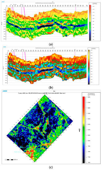
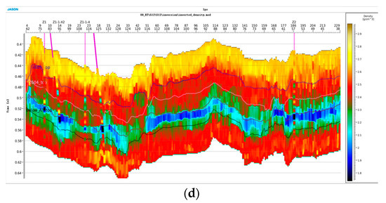
Figure 8.
Prestack simultaneous inversion test: (a) section of P-wave impedance; (b) section of S-wave impedance; (c) plan of P-wave impedance; (d) section of postwave impedance.
3.4. Prestack Geostatistical Inversion Test
At the same time, prestack AVO inverses the accurate rock elastic parameter volumes under seismic resolution, such as P-wave impedance and P-wave velocity ratio. These data volumes conform to the petrophysical model and are faithful to the seismic response, but their longitudinal resolution is limited by the seismic resolution.
For further geological research [29], when seismic data information cannot meet the needs of reservoir research, it is necessary to further organically integrate regional geological concepts and well information with seismic data, so as to make full use of the high predictability of earthquakes horizontally and the high resolution of wells vertically.
The prestack random inversion [30,31] workflow makes full use of logging data and geological statistical data and, on the basis of well matching with seismic data, generates horizontally continuous high-resolution P-wave impedance, S-wave impedance (or P-wave velocity ratio), density body, and discrete lithologic body. This workflow can usually solve the problems of the thin layer below the seismic resolution and lithology multiplicity of single seismic attribute superposition, and improve the resolution of data volume such as porosity and permeability.
Prestack random inversion combines constrained sparse pulse inversion with random simulation technology to become a brand-new random inversion algorithm. By combining seismic data, prior sedimentary facies information, geological statistics information, logging curve, probability density function, and variogram information, a strict probability distribution model is defined.
As shown in Figure 9, the probability density function and variation function are obtained by analyzing logging data and prior geological information. Secondly, according to the probability distribution function (PDF), the statistically correct sample point set is obtained, that is, the kind of results that can be obtained according to the probability distribution function. The built-in constrained sparse pulse inversion engine ensures that within the effective bandwidth of seismic data, the inversion result is to reproduce a real reservoir parameter with clear lithologic bodies with sharp edges at appropriate positions and more details.
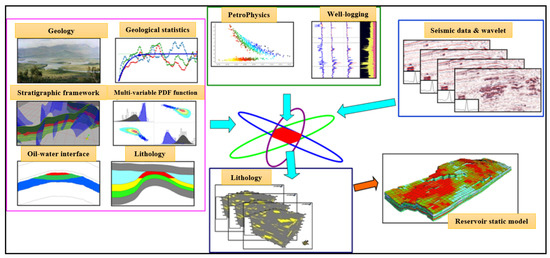
Figure 9.
Schematic diagram of prestack geostatistical inversion workflow.
Thanks to the previous test basis of poststack wave impedance inversion, poststack geostatistical inversion, and prestack simultaneous inversion, we have a better understanding of the vertical and horizontal variation functions of the seismic, wavelet, horizon framework, and geostatistical parameters in this area. Therefore, this prestack geostatistical inversion parameter test is more targeted, and the inversion results are of good quality, as shown in Figure 10a–c. The prestack geostatistical inversion of P-wave impedance (AI), S-wave impedance (SI), and density (DEN) has good correlation with wells, reasonable vertical resolution, clear boundary of geological body, high precision, mainly density result, good stability, and vertical resolution.
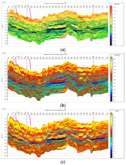
Figure 10.
Prestack geostatistical inversion test result: (a) section of AI; (b) section of SI; (c) section of DEN.
Therefore, the prestack geostatistical inversion results (lithology, AI, SI, DEN, and their combination operations) are preferred for quantitative interpretation of parameters such as lithology, oil–gas potential, in situ stress, and media structure.
4. Results
4.1. Quantitative Interpretation Technology of Coal Seam Thickness
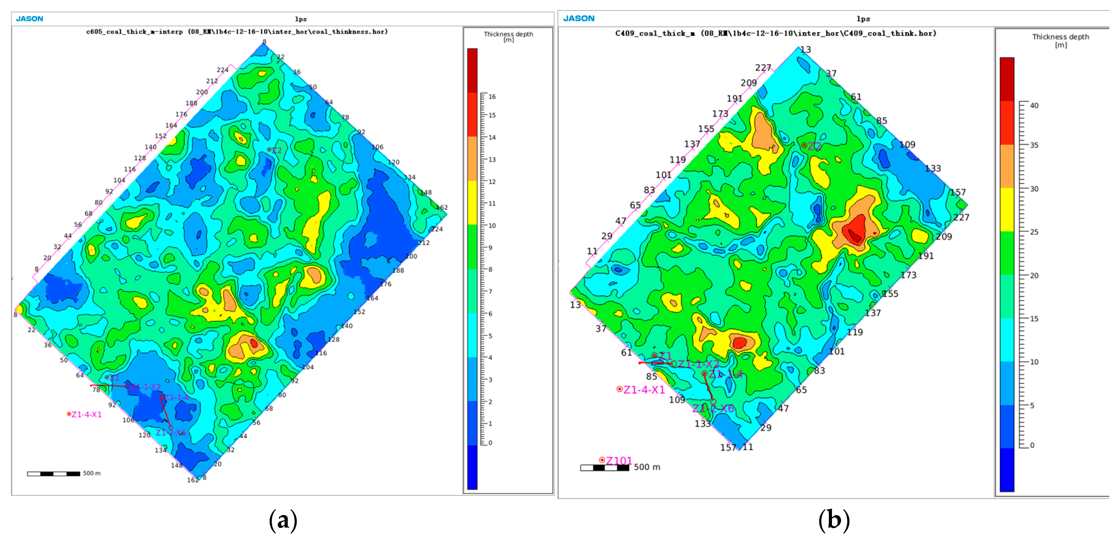
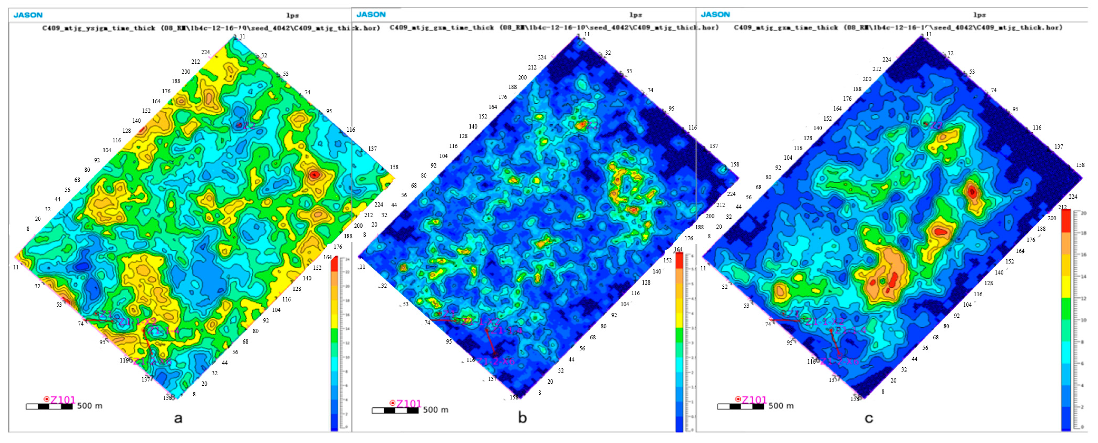
The interpretation of coal seam thickness parameters is based on the inversion of three-dimensional lithologic bodies by prestack geostatistics. First, among multiple realizations, the realization with the best coincidence rate with well, seismic, and geological knowledge is selected, and the inversion coal seam thicknesses of C605-C504 and C409-C406 intervals are counted, respectively.
As shown in Figure 11a, in the enrichment section of the coal seam (upper coal seam) in the C605-C504 interval, the thickness area of the coal seam is located in the middle of the work area, with the southern belt running in the near northwest direction and the northern belt running in the near northeast direction. As shown in Figure 11b, in the enrichment section of the coal seam (lower coal seam) in the C409-C406 interval, the thick area of coal seam thickness is located in the middle of the work area. Except for the area with complex structures, other areas with relatively uniform structures have a relatively stable thick coal seam distribution. It can be seen that the prediction results are consistent with the geological law. The total thickness of the lower coal seam is relatively thick, reaching more than 40 m locally, most of which exceeds 15 m. The total thickness of the upper coal seam is relatively thin, over 15 m locally, 6–10 m in most areas, and less than 4 m in about 1/5 of areas.

Figure 11.
Inversion map of coal seam thickness: (a) C605-C504; (b) C409-C406.
4.2. CBM Content Prediction Technology
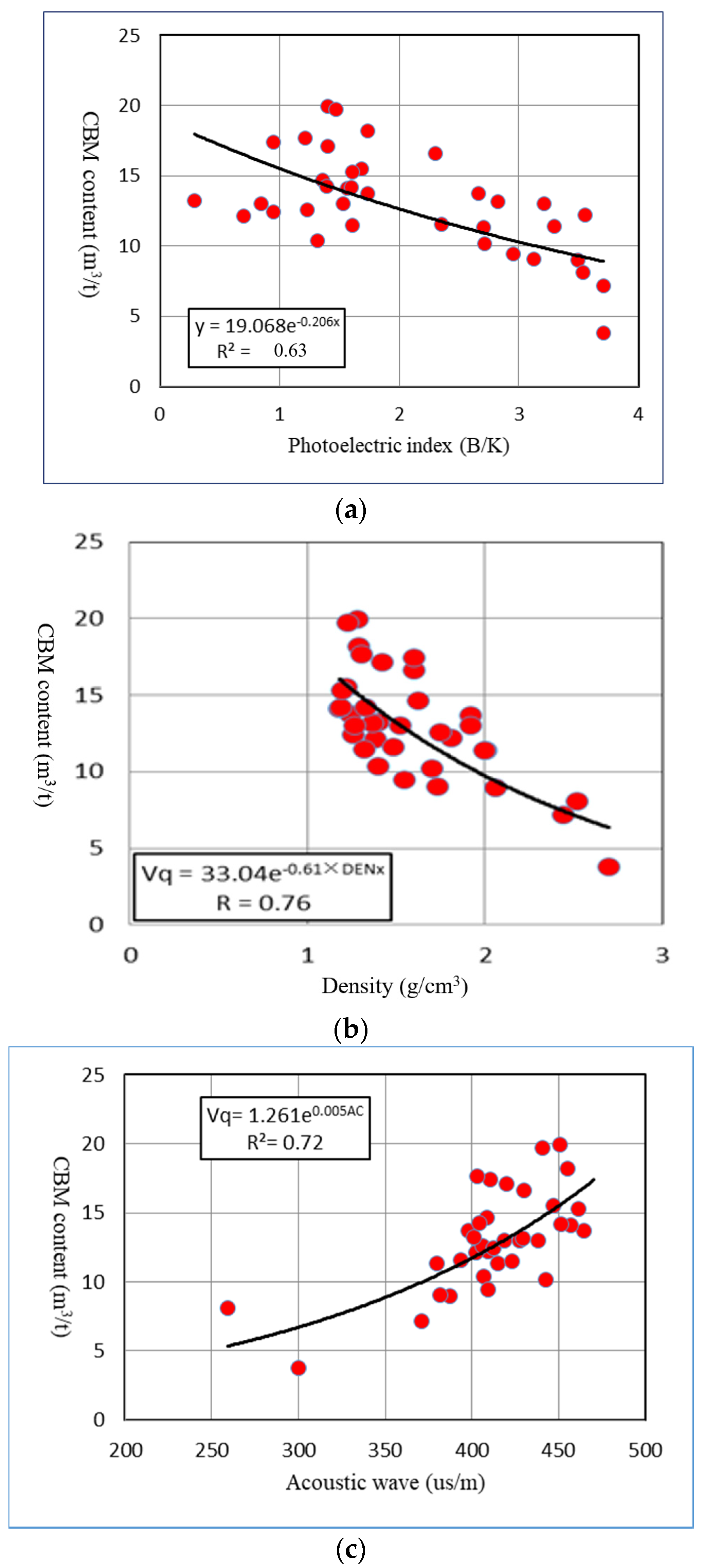
According to the report “Research on Guizhou CBM Logging Evaluation Technology”, compiled in 2016, predecessors used the experimental data of 43 coal cores from 6 wells in the Liupanshui area, established the calculation model of coal composition parameters through coal core calibration logging curves adopting the method of mathematical statistics, and analyzed the correlation between gas content and various logging parameters. The logging curve characteristics in the Liupanshui area have a good correlation with the test results of gas content in the coal core, and the gas content has a good correlation with photoelectric index, density, and sound wave. The correlation coefficients are 0.63, 0.76, and 0.72, respectively (as shown in Figure 12a–c).
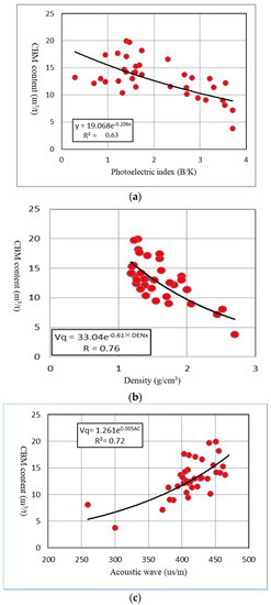
Figure 12.
Relationship between CBM content and (a) photoelectric index, (b) density, and (c) acoustic wave: (a) CBM content and photoelectric index; (b) CBM content and density; (c) CBM content and acoustic wave.
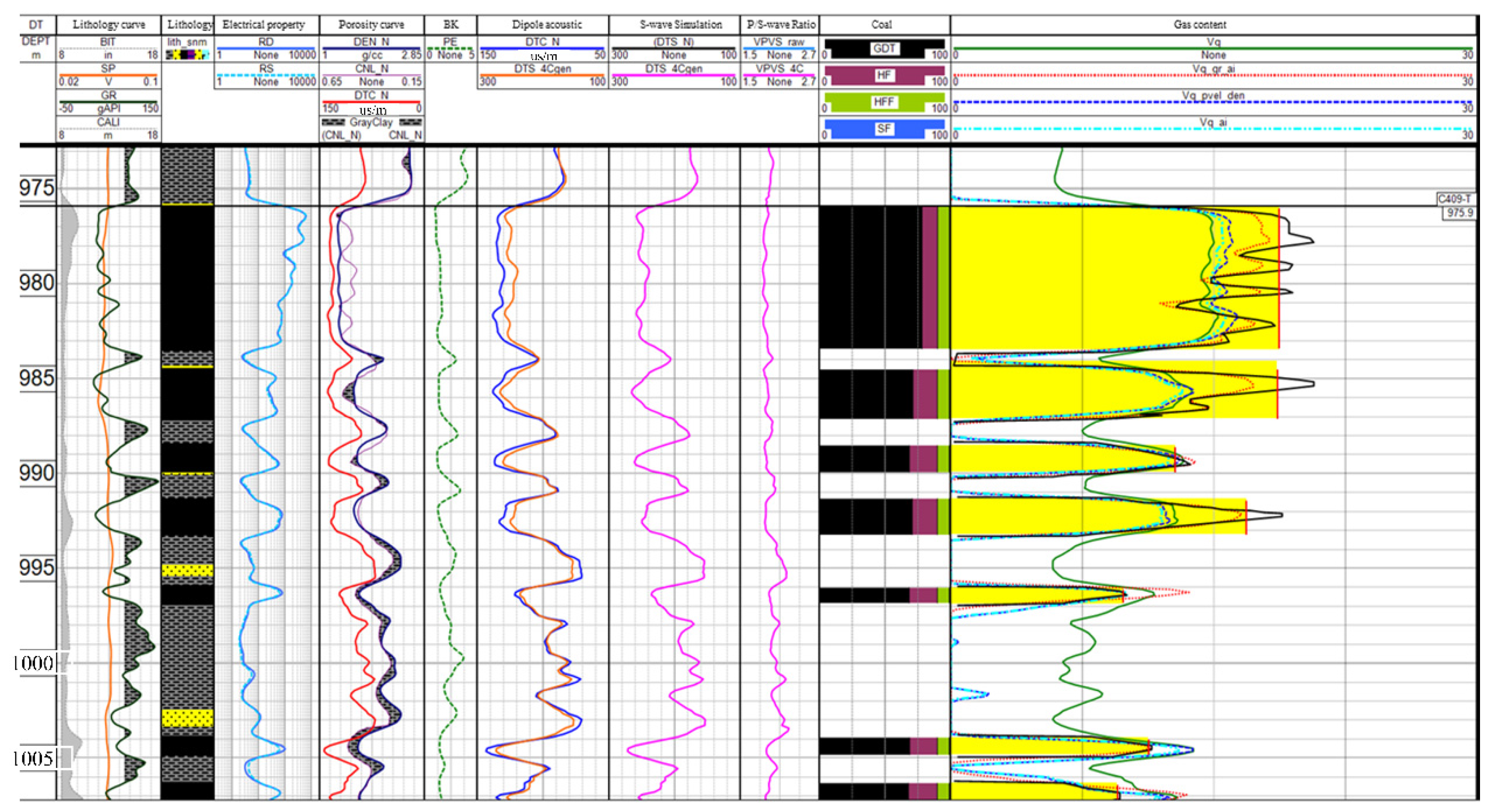
By consulting the logging interpretation report in this area, the following formula is used in the report: VQ = EXP (4.493 + 0.002408 × AC − 0.412 × DEN)/10, where AC and DEN, respectively, represent the acoustic time difference and density curves of logging, but the gas content interpretation result curve (black curve in Figure 13) provided by logging obviously contains a gamma (GR) curve. Because the above equation provided in the logging interpretation report is used, only the AC and DEN curves are used to calculate the gas content (green curve in Figure 13), and the correlation with the gas content curve provided by the logging interpretation is only 83%. If the GR curve is added, three parameters are used to calculate the gas content, as shown by the red curve in Figure 13, and the correlation coefficient with the gas content result curve provided by the logging interpretation reaches 91%, so observe the details of the gas content interpretation of the C409 coal seam. It also coincides with the shape of the GR curve, indicating that the calculation formula of the gas content interpretation model provided in the logging interpretation report does not coincide with the gas content interpretation curve in the logging interpretation result curve. Considering that the correlation coefficient between the GR curve and the coalbed methane gas content is not high, only 38%, and the GR curve is not sensitive to the coalbed methane gas content from the logging mechanism, introducing the GR curve to calculate the coalbed methane gas content will introduce uncertainty.
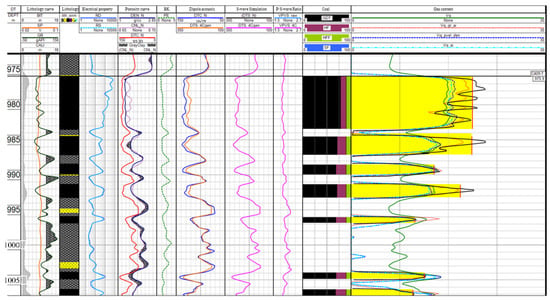
Figure 13.
Comparison between CBM content prediction and measured curve.
Therefore, it is necessary to re-establish the CBM logging interpretation model. Based on the elastic parameter acoustic wave × density = longitudinal wave impedance (AI), which is the most commonly used elastic parameter, the calculation model of the gas content is re-fit: Vgas = 28.8241 − 0.00441113 × AI. (Figure 13 cyan curve). The uncertainty caused by the GR curve is avoided, and only the elastic curve is included, which is beneficial to obtain the spatial distribution characteristics of the gas content by seismic inversion prediction. According to the numerical value of the gas content interpretation of each coal seam in the logging interpretation result table, the gas content interpreted by the new model is in good agreement with the logging interpretation result.
The conversion formula of the sensitive factor of the coalbed methane gas content is established by elastic parameter AI: Vgas = 28.8241 − 0.00441113 × AI, which has high sensitivity. Based on this conversion relationship, the longitudinal wave impedance obtained by seismic inversion can be converted into a three-dimensional volume of the coalbed methane gas content, and the quantitative interpretation of the coalbed methane gas content in this area can be carried out.
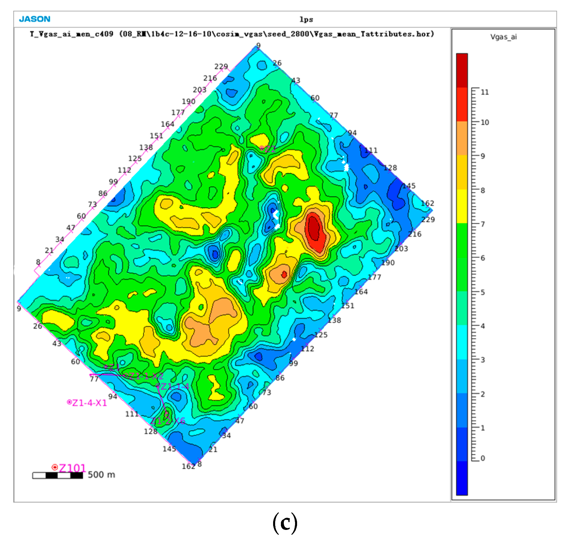
As shown in Figure 14a, the profile of the gas content in the three-dimensional well connection by using longitudinal wave impedance conversion shows that the gas content is in high agreement with the gas content interpreted by logging at well points, and the variation between wells can conform to the law of seismic data, with high longitudinal resolution and certain response to thin layers. It can be seen from the figure that the areas with high gas content are mainly concentrated in the middle of the lower coal seam. Based on this three-dimensional data volume, the gas content plans of the C605-C504 and C409-C406 layers (as shown in Figure 14b,c) are calculated, respectively. As shown in Figure 14b, the high-value area of gas content in the C605-C504 interval is distributed in the south–central part of the work area, showing a strip-like distribution with a nearly north–south trend. As shown in Figure 14c, the area with high gas content in the C409-C406 interval is distributed in the middle of the work area, with relatively low gas content near the fault and relatively high gas content in areas where the fault is undeveloped. The predicted results are in good agreement with geological laws. The local gas content in the C605-C504 interval can reach 5 t/m3, and the gas content In most areas is 1–5 t/m3. The local gas content of the C409-C406 interval exceeds 11, and the gas content of most areas is 4–11 t/m3, which is much higher than that of the C605-C504 interval coal seam.
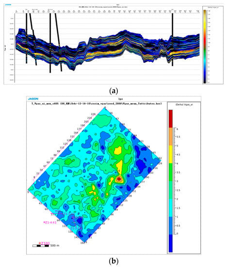
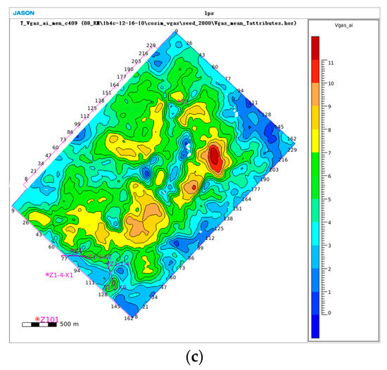
Figure 14.
CBM content prediction result: (a) section of CBM content prediction based on prestack geostatistical inversion; (b) plan of C605-C504; (c) plan of C409-C406.
4.3. Coal Body Structure Prediction Technology
The quantitative interpretation template of the coal structure is established by the elastic parameters acoustic time difference (DT) (reciprocal of velocity) and density (DEN). This prestack geostatistical inversion can directly invert the velocity and density 3D body, which form the basis of the quantitative interpretation of the coal structure.
Take the reciprocal of the acoustic time difference and convert it into P-wave velocity (VEL) in m/s, and the second elastic parameter density in g/cm3. The interpretation version of the coal structure is as follows: primary structure coal: DEN ≥ 1.5 and VEL ≥ 2438, fragmented coal: 1.3 ≤ DEN < 1.5 and 2257 ≤ VEL < 2438, structure coal: DEN < 1.3 and VEL < 2257. Using the above explanation template, the thickness of the distribution of the three types of coal bodies in C605-C504 and C409-C406 in this area was quantitatively explained.
As shown in Figure 15, the coal bodies; thickness distribution plan of C605-C504 is predicted. The thickness of the primary structure coal is the largest among the three types, and the thickness area is mainly distributed in the west of the work area, showing a strip-like distribution in the axial direction near the northwest. In comparison, the thickness distribution of the other two types of coal structure is relatively scattered. As shown in Figure 16, the prediction plan of the thickness distribution of coal bodies in the C409-C406 interval shows that the thickness of the primary structure coal is also the largest among the three types. The thick value areas are mainly distributed in the areas with few fractures in the work area, the fragmented coal is scattered, and the structure coal is mainly distributed in the south of the work area in a banded pattern.
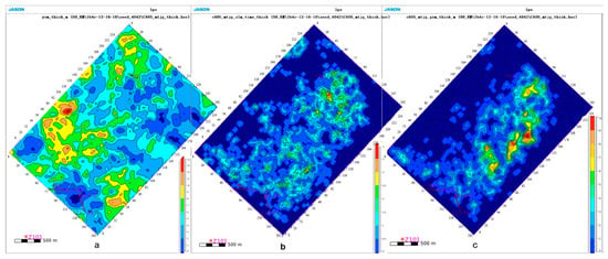
Figure 15.
Plan of coal structure thickness distribution predicted by inversion of C605-C504: (a) primary structure coal; (b) fragmented coal; (c) structure coal.

Figure 16.
Plan of coal structure thickness distribution predicted by inversion of C409-C406: (a) primary structure coal; (b) fragmented coal; (c) structure coal.
4.4. In Situ Stress Prediction Technology
The following describes the method of in situ stress prediction based on seismic data from three aspects: reflection coefficient inversion, seismic curvature attribute, and petrophysical modeling.
4.4.1. In Situ Stress Prediction Technology Based on Reflection Coefficient Inversion
Tiğrek et al. [11] established the objective function by analyzing the relationship between the PP wave reflection coefficient, the PS wave reflection coefficient, and in situ stress. By optimizing the function iteratively, the dynamic parameters of the underground medium can be inverted. Tiğrek et al. [11] pointed out that the static parameters of the underground medium can better reflect the stress state of the underground medium. First, the ratio of dynamic and static parameters in the target area should be obtained through experimental measurement, and the static parameters should be obtained on the basis of reflection coefficient inversion. Then, a geomechanical model should be established by using the static parameters. Finally, the stress distribution of the underground medium should be calculated based on this model.
4.4.2. In Situ Stress Prediction Technology Based on Curvature Attributes
The curvature of strata is closely related to strain, and Hooke’s law relates strain and stress together. Hunt et al. [32] established the relationship between formation curvature and in situ stress. The product of Young’s modulus and curvature can be used to approximate the stress properties of the formation and provide a reliable basis for the prediction of fracture density.
Under the assumption of thin-plate theory, He et al. [33] derived the expression of in situ stress based on curvature. Young’s modulus and Poisson’s ratio of the underground medium are obtained by seismic inversion, and the curvature attribute is calculated from seismic horizon data so that the in situ stress distribution of the underground medium can be predicted.
Xiong et al. [34] also gave a method of in situ stress prediction based on curvature: first, Young’s modulus and Poisson’s ratio of the underground elastic parameters are inverted by using seismic data. Then, the velocity of the underground medium layer is obtained by using seismic data and velocity analysis, and then the formation pressure is calculated. Subsequently, the curvature attribute is calculated by using prestack seismic data and horizon data, and the horizontal tectonic strain is calculated by using the curvature attribute. Finally, the above calculation results are substituted into the linear isotropic combined spring model to predict the underground stress distribution. The calculated Young’s modulus is a dynamic one [35,36].
4.4.3. In Situ Stress Prediction Technology Based on Rock Physical Model
The rock physical model establishes the relationship between seismic data and reservoir parameters. Through comprehensive analysis of seismic data and other geological and logging data, physical parameters such as porosity and lithology in the work area can be obtained. Based on this, a petrophysical model can be established, and the stiffness matrix of the underground medium can be obtained, thus realizing the prediction of the in situ stress distribution. Zhang et al. [37] studied the prediction of in situ stress based on the petrophysical model. Taking shale as an example, first, according to seismic data and other prior information, the parameters such as minerals and porosity in the work area are comprehensively analyzed, and a petrophysical model is established. Then, based on the petrophysical model, the stiffness matrix of the underground medium is calculated, and the P-wave velocity and S-wave velocity are selected. Shale can be regarded as a VTI medium, so the VTI medium model can be used to predict in situ stress.
Based on the above investigation on the method of seismic prediction of in situ stress, combined with the geological characteristics of this area, the method of curvature and Young’s modulus combined prediction of in situ stress is selected to predict the in situ stress in this area.
Firstly, the curvature of the C605-C504 and C409-C406 layers in this area is calculated. As shown in Figure 17, the maximum positive curvature of the C605 top surface and the C409 top surface curvature plan are in good agreement with the fracture.
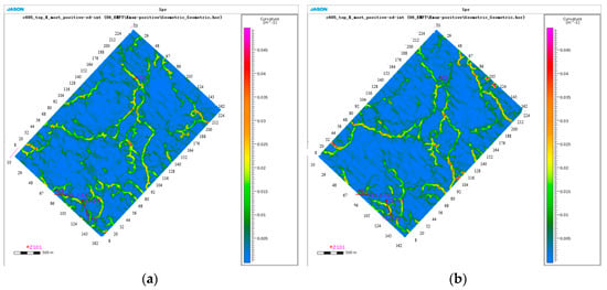
Figure 17.
Plan of maximum positive curvature of coal seam top boundary: (a) C605-C504; (b) C409-C406.
Next, Young’s modulus of C605-C504 and C409-C406 layers in this area is calculated. The main parameters used are P-wave velocity, S-wave velocity, and density, which are directly obtained by prestack geostatistical inversion, as shown in Figure 16, the C605-C504 and C409-C406 layers, the low Young’s modulus area (blue area in Figure 18), and fracture.
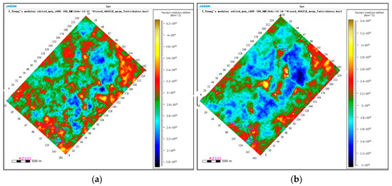
Figure 18.
Plan of mean Young’s modulus: (a) C605-C504; (b) C409-C406.
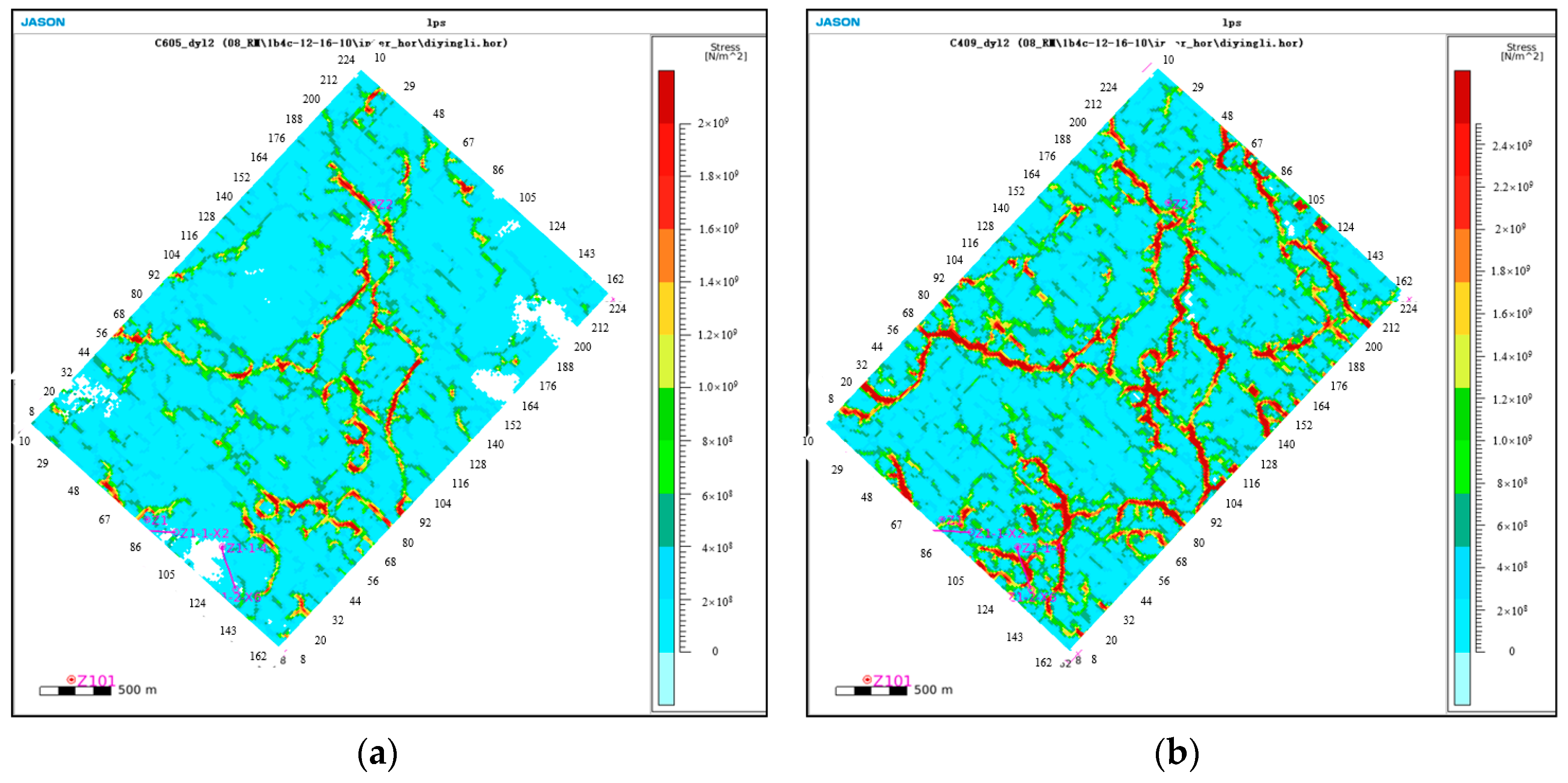
After obtaining the curvature and Young’s modulus, the coal seam thickness of the main coal seam development section predicted by inversion is used to calculate the in situ stress. The result is as shown in Figure 19. The high-value area of in situ stress is consistent with the distribution height of faults, and the high-value area of in situ stress can be avoided by considering avoiding faults within 200 m in the subsequent well location deployment.

Figure 19.
Plan of in situ stress: (a) C605-C504; (b) C409-C406.
5. Discussion: CBM Sweet-Spot Comprehensive Evaluation Technology
Through seismic inversion prediction, several evaluation parameters of CBM, such as coal seam thickness, coal seam CBM content, coal body structure, in situ stress, etc., are obtained. If the above parameters are comprehensively utilized, the real sweet spot of CBM development can be predicted, which will make the predicted sweet spot more practical and focused.
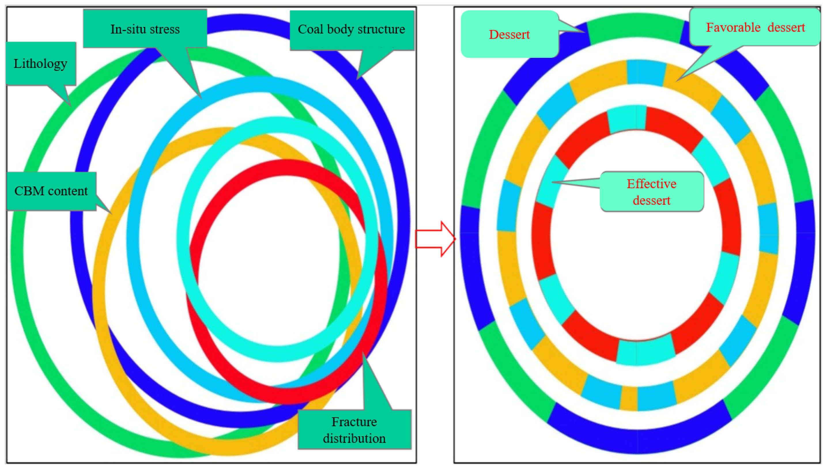
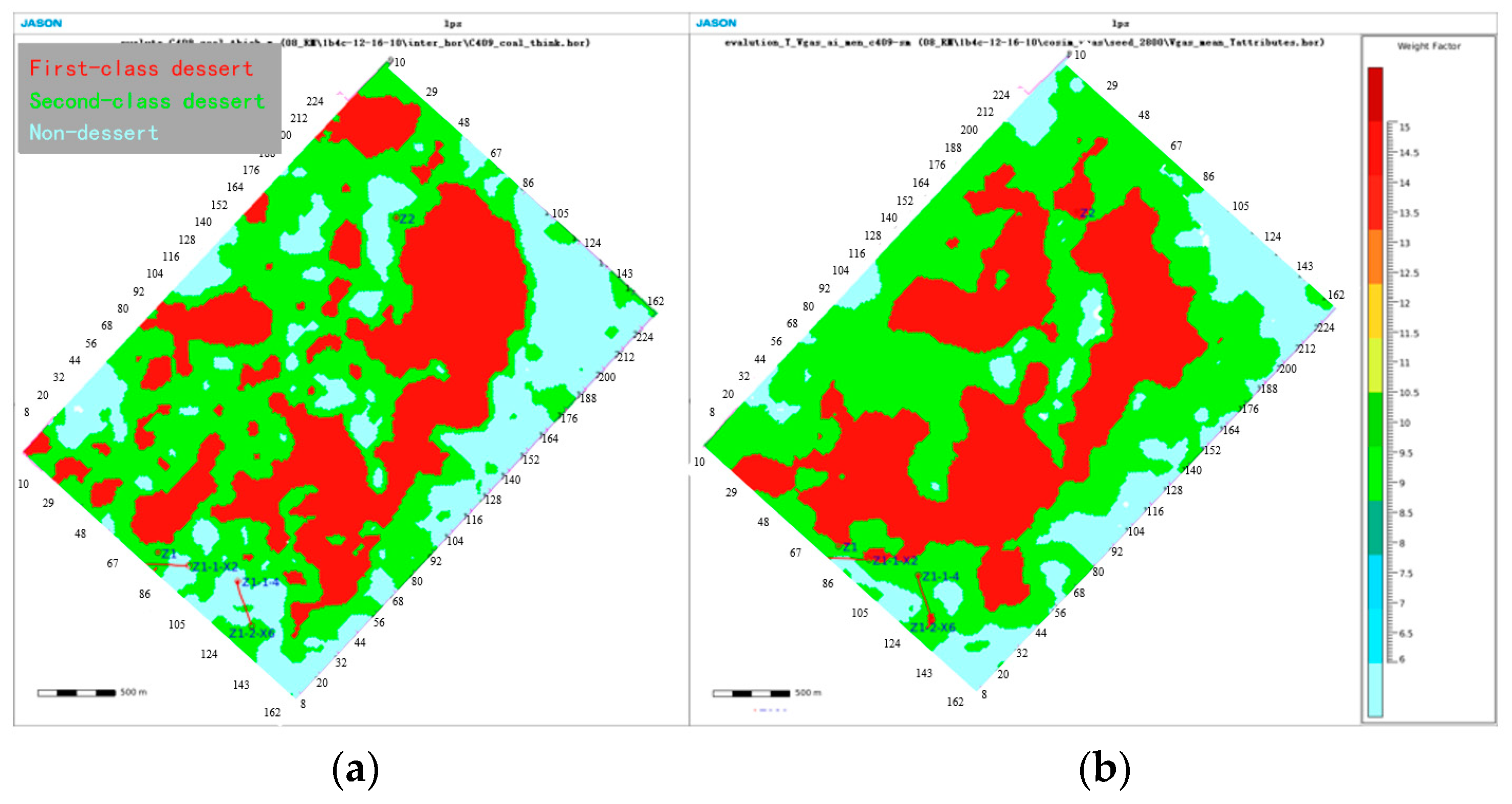
According to the experience of sweet-spot evaluation in the past, the simple stacking of evaluation parameters cannot find out the real sweet spot. Only by giving each parameter an appropriate weight can we focus on the real effective sweet-spot area. Therefore, based on the previous experience of CBM development in Guizhou Province, the evaluation parameters are determined. Based on this understanding, this study innovatively puts forward the multifactor weighted step-by-step evaluation method (as shown in Figure 20) to comprehensively evaluate the distribution characteristics of the CBM sweet spot. Specific evaluation parameters are shown in Table 2.
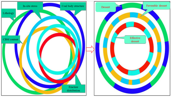
Figure 20.
Schematic diagram of the multifactor weighted step-by-step evaluation method.

Table 2.
Parameter table of multiparameter CBM sweet-spot evaluation for reservoir prediction.
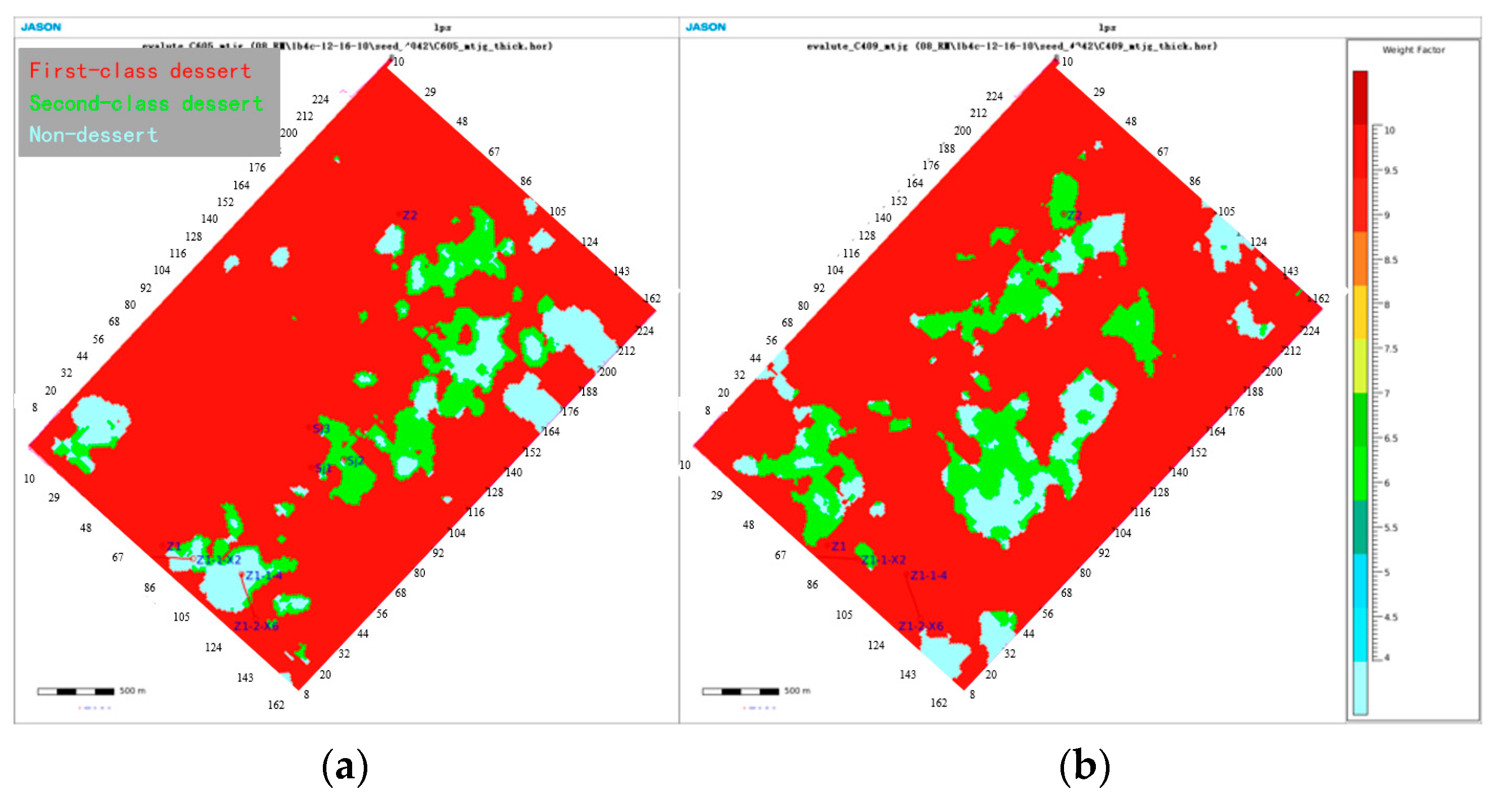
Based on this standard, the single-parameter sweet-spot plan is calculated for the three evaluation parameters of coal seam thickness, gas content, and coal body structure. As shown in Figure 21, the sweet-spot areas of coal seam thickness are mainly distributed in the middle of the work area, showing a strip-like distribution. As shown in Figure 22, the sweet spots of coal seam CBM content are mainly distributed in the south–central part of the work area, which is distributed in strips. As shown in Figure 23, the coal structure of the coal seam is mainly primary structure coal, while the other two types account for a relatively small proportion.

Figure 21.
Sweet-spot map based on coal seam thickness: (a) C605-C504; (b) C409-C406.

Figure 22.
Sweet-spot map based on coal seam CBM content: (a) C605-C504; (b) C409-C406.

Figure 23.
Sweet-spot map based on coal body structure: (a) C605-C504; (b) C409-C406.
After weighing each evaluation parameter separately, the plan of sweet-spot evaluation weight factor with multiple parameters is formed by the method of accumulation.
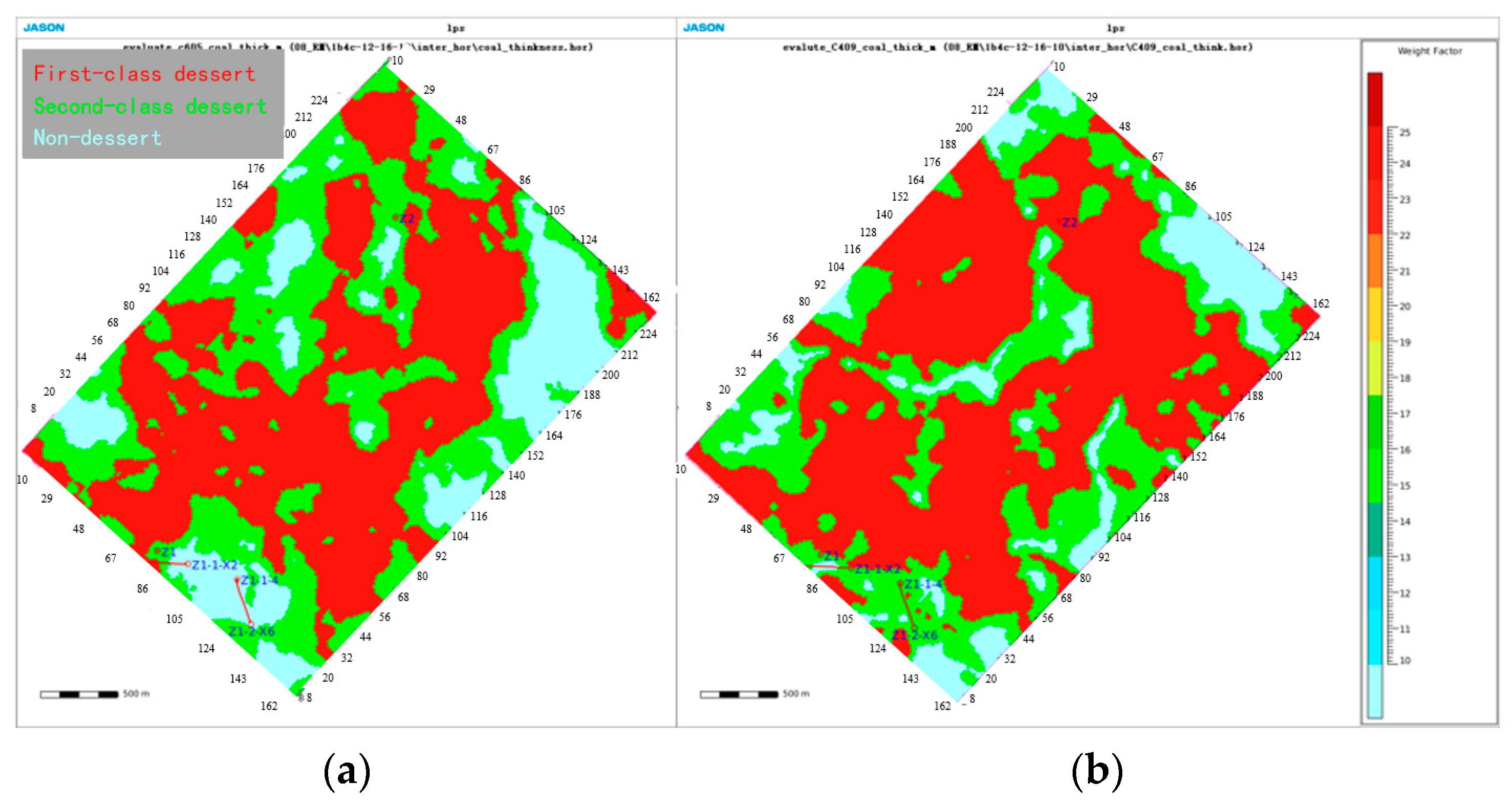
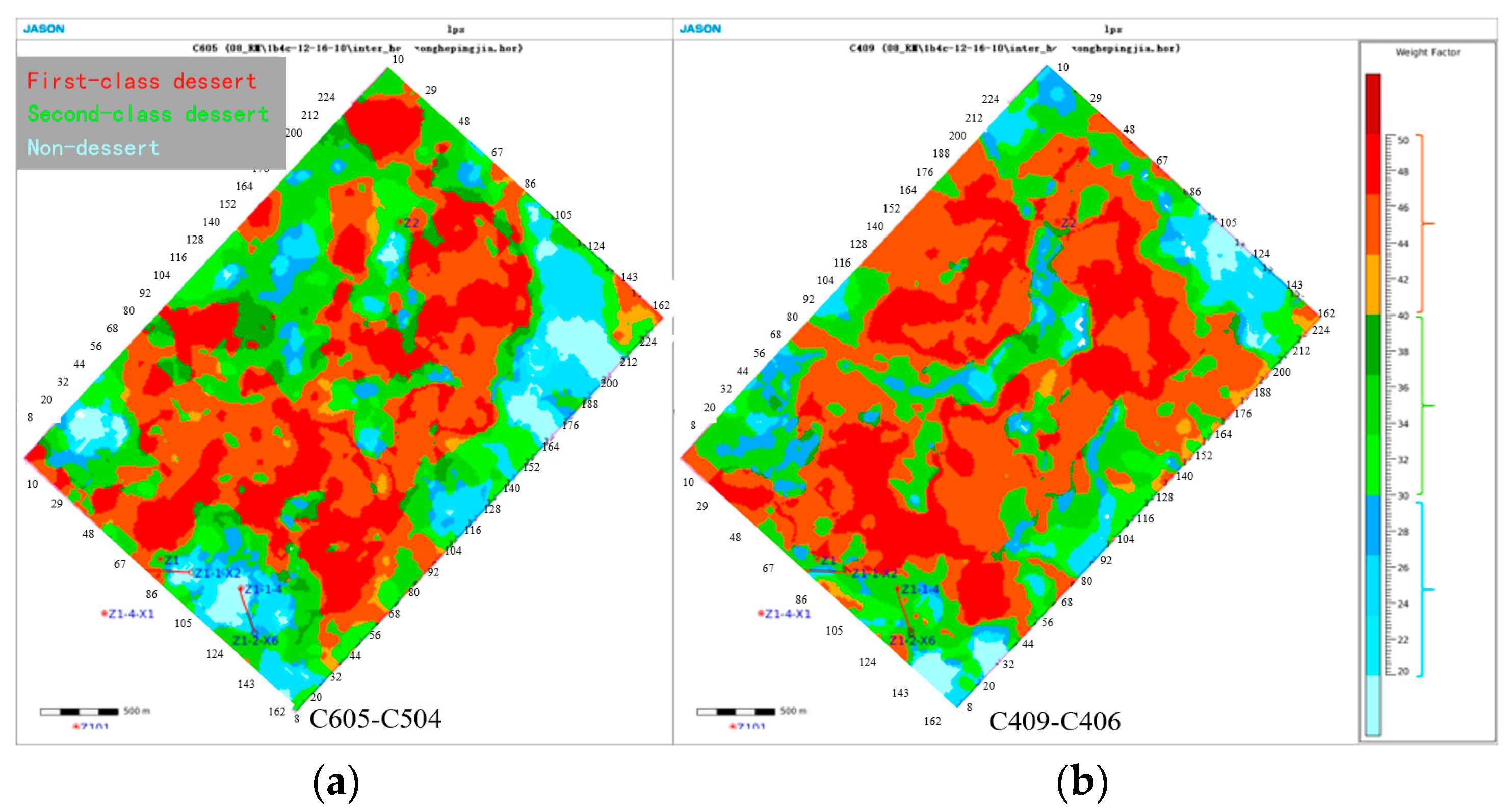
As shown in Figure 24, the comprehensive sweet-spot prediction plan of CBM in this area combines the characteristics of classified evaluation of three evaluation parameters, namely, coal seam thickness, CBM content, and coal body structure. It can be seen that the evaluation parameters of sweet spots in this plan range from 20 to 50, with 10 as an equal part. Those with scores between 40 and 50 are classified into first-class sweet spots, those with scores between 30 and 40 are classified into second-class sweet spots, and those with scores between 20 and 30 are classified into non-sweet spots. From the comprehensive sweet-spot plan, it can be seen that the characteristics of the three evaluation parameters of coal seam thickness, CBM content, and coal body structure are reflected, and each has its own emphasis due to the size of the weight value, which is a reasonable division scheme. The C409 coal seam has the largest distribution area in the desert area.
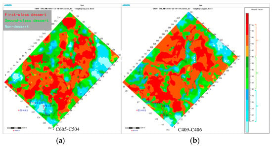
Figure 24.
Comprehensive sweet-spot evaluation map of main coal seam: (a) C605-C504; (b) C409-C406.
6. Conclusions
(1) In the aspect of data interpretation, while extending the traditional technology to the research types of coalbed methane, it also actively explores new technologies and methods applicable to coalbed methane, especially in the quantitative prediction methods of coal seam thickness, CBM content, coal structure, in situ stress, and other parameters.
(2) Based on logging evaluation and petrophysics, a series of three-highs quantitative prediction technologies for CBM sweet spots, featuring high precision, high resolution, and high coincidence, is explored by applying various reservoir prediction methods at the same time.
(3) In addition, the multiparameter weighted step-by-step evaluation method based on inversion is innovatively put forward in the comprehensive evaluation of multiparameter sweet spots, which makes the prediction of sweet spots of CBM more focused, effective, and practical, and the distribution law of sweet spots is more in line with the geological law, providing sufficient basis for the subsequent well location deployment. Based on this method, the C409 coal seam was selected as the sweet spot.
Author Contributions
Conceptualization, Y.W. and W.L.; methodology, L.Z. and Z.W.; software, S.Y.; validation, X.Z., Z.G. and Z.W.; formal analysis, X.Z. and L.Z.; investigation, L.Z. and Y.W.; resources, Y.W. and L.Z.; data curation, S.Y. and X.Z.; writing—original draft preparation, Y.W.; writing—review and editing, X.Z.; supervision, W.L.; funding acquisition, Y.W. and L.Z. All authors have read and agreed to the published version of the manuscript.
Funding
This work was supported by the Guizhou Provincial Geological Exploration Fund under grant 208-9912-JBN-UTS0, and 52000021MGQSE7S7K6PRP, and Guizhou Provincial Fund Project under grant Nos. (2022)ZD001.
Data Availability Statement
Not applicable.
Conflicts of Interest
The authors declare no conflict of interest.
References
- Zhang, X.; Liu, W.; Chen, J.; Jiang, D.; Fan, J.; Daemen, J.; Qiao, W. Large-scale CO2 disposal/storage in bedded rock salt caverns of China: An evaluation of safety and suitability. Energy 2022, 249, 123727. [Google Scholar] [CrossRef]
- Krivoshchekov, S.; Kochnev, A.; Kozyrev, N.; Ozhgibesov, E. Factoring Permeability Anisotropy in Complex Carbonate Reservoirs in Selecting an Optimum Field Development Strategy. Energies 2022, 15, 8866. [Google Scholar] [CrossRef]
- Zhang, M.; Li, Z.; Liu, Q.; Yi, J.; Li, K. A study on the characteristics of seismic wave propagation in fractured marlstone reservoirs based on mechanical principles. Arab. J. Geosci. 2021, 14, 1437. [Google Scholar] [CrossRef]
- Gyulai, Á.; Baracza, M.K.; Szabó, N.P. On the application of combined geoelectric weighted inversion in environmental exploration. Environ. Earth Sci. 2014, 71, 383–392. [Google Scholar] [CrossRef]
- Rodrigues, P.M.S.M.; Antão, A.M.M.C.; Rodrigues, R. Evaluation of the impact of lithium exploitation at the C57 mine (Gonçalo, Portugal) on water, soil and air quality. Environ. Earth Sci. 2019, 78, 533. [Google Scholar] [CrossRef]
- Wang, Y. Seismic impedance inversion using l1-norm regularization and gradient descent methods. J. Inverse Ill-Posed Probl. 2011, 18, 823–838. [Google Scholar] [CrossRef]
- Wu, H.; Li, S.; Chen, Y.; Peng, Z. Seismic impedance inversion using second-order overlapping group sparsity with A-ADMM. J. Geophys. Eng. 2019, 17, 97–116. [Google Scholar] [CrossRef]
- Wu, B.; Meng, D.; Zhao, H. Semi-Supervised Learning for Seismic Impedance Inversion Using Generative Adversarial Networks. Remote Sens. 2021, 13, 909. [Google Scholar] [CrossRef]
- Gong, W.; Wen, X.; Zhou, D. Characteristics and Seismic Identification Mode of Ultra-Deep Carbonate Fault-Controlled Reservoir in Northwest China. Energies 2022, 15, 8598. [Google Scholar] [CrossRef]
- Ma, N.; Yin, X.Y.; Sun, C.Y.; Zong, Z.Y. The in-situ stress seismic prediction method based on the theory of orthorhombic anisotropic media. Chin. J. Geophys. 2017, 60, 4766–4775. [Google Scholar]
- Tiğrek, S.; Slob, E.; Dillen, M.; Cloetingh, S.; Fokkema, J. Linking dynamic elastic parameters to static state of stress: Toward an integrated approach to subsurface stress analysis. Tectonophysics 2005, 397, 167–179. [Google Scholar] [CrossRef]
- Kumar, R.; Das, B.; Chatterjee, R.; Sain, K. A methodology of porosity estimation from inversion of post-stack seismic data. J. Nat. Gas Sci. Eng. 2016, 28, 356–364. [Google Scholar] [CrossRef]
- Ali, A.; Alves, T.M.; Saad, F.A.; Ullah, M.; Toqeer, M.; Hussain, M. Resource potential of gas reservoirs in South Pakistan and adjacent Indian subcontinent revealed by post-stack inversion techniques. J. Nat. Gas Sci. Eng. 2018, 49, 41–55. [Google Scholar] [CrossRef]
- Negm, S.A.; Khalil, M.H.; Bakr, A. Gas prediction through the LMR method using post-stack inversion and multi-attributes, F3 cube, North Sea, Netherlands. Arab. J. Geosci. 2020, 13, 674. [Google Scholar] [CrossRef]
- Morozov, I.B.; Ma, J. Accurate poststack acoustic-impedance inversion by well-log calibration. Geophysics 2009, 74, R59–R67. [Google Scholar] [CrossRef]
- Meng, D.; Wu, B.; Wang, Z.; Zhu, Z. Seismic Impedance Inversion Using Conditional Generative Adversarial Network. IEEE Geosci. Remote Sens. Lett. 2021, 19, 1–5. [Google Scholar] [CrossRef]
- Tang, Q.; Tang, S.; Luo, B.; Luo, X.; Feng, L.; Li, S.; Wu, G. Seismic Description of Deep Strike-Slip Fault Damage Zone by Steerable Pyramid Method in the Sichuan Basin, China. Energies 2022, 15, 8131. [Google Scholar] [CrossRef]
- Xu, H. Geological Theory and Technology for Coalbed Methane Development with Thin and Medium Coal Seam Zones in Guizhou; China University of Mining and Technology: Xuzhou, China, 2012. [Google Scholar]
- Yang, R.; Tang, X. Coal-bearing Strata Characteristic Analysis in Lupanshui Coalfield, Guizhou Province. Coal Geol. China 2014, 26, 28–32. [Google Scholar]
- Dai, R.; Zhang, F.; Yin, C.; Hu, Y. Multi-trace post-stack seismic data sparse inversion with nuclear norm constraint. Acta Geophys. 2021, 69, 53–64. [Google Scholar] [CrossRef]
- Karslı, H.; Güney, R.; Senkaya, M. Post-stack high-resolution deconvolution using Cauchy norm regularization with FX filter weighting. Arab. J. Geosci. 2017, 10, 551. [Google Scholar] [CrossRef]
- Yu, B.; Zhou, H.; Wang, L.; Liu, W. Prestack Bayesian statistical inversion constrained by reflection features. Geophysics 2020, 85, R349–R363. [Google Scholar] [CrossRef]
- Sun, Y. Integrated research of seismic inversion, geological modeling and reservoir simulation based on geostatistical inversion and its applications. Acta Geophys. 2021, 69, 1789–1797. [Google Scholar] [CrossRef]
- Durrani, M.Z.; Talib, M.; Ali, A.; Sarosh, B.; Rahman, S.A. Characterization of carbonate reservoir using post-stack global geostatistical acoustic inversion approach: A case study from a mature gas field, onshore Pakistan. J. Appl. Geophys. 2021, 188, 104313. [Google Scholar] [CrossRef]
- Lavaud, B.; Kabir, N.; Chavent, G. Pushing AVO Inversion Beyond Linearized Approximation. J. Seism. Explor. 1999, 8, 279–302. [Google Scholar] [CrossRef]
- Booth, A.D.; Emir, E.; Diez, A. Approximations to seismic AVA responses: Validity and potential in glaciological applications. Geophysics 2015, 81, WA1–WA11. [Google Scholar] [CrossRef]
- Hu, G.-Q.; Liu, Y.; Wei, X.-C.; Chen, T.-S. Joint PP and PS AVO inversion based on Bayes theorem. Appl. Geophys. 2011, 8, 293–302. [Google Scholar] [CrossRef]
- Simmons, J.L. Waveform-based AVO inversion and AVO prediction-error. Geophysics 2012, 61, 1575. [Google Scholar] [CrossRef]
- Oh, S. Geostatistical integration of seismic velocity and resistivity data for probabilistic evaluation of rock quality. Environ. Earth Sci. 2013, 69, 939–945. [Google Scholar] [CrossRef]
- Dennis, V.D.B.; Verdel, A.; Wapenaar, K. Ray-based stochastic inversion of prestack seismic data for improved reservoir characterization. Geophysics 2009, 74, R85–R97. [Google Scholar]
- Srivastava, R.P.; Sen, M.K. Stochastic inversion of prestack seismic data using fractal-based initial models. Geophysics 2010, 75, R47–R59. [Google Scholar] [CrossRef]
- Hunt, L.; Beshry, B.; Chopra, S.; Webster, C. Determination of target-oriented parameters for computation of curvature attributes. Interpretation 2018, 6, T485–T498. [Google Scholar] [CrossRef]
- He, Y.; He, Z.; Xiong, X. Fault Identification Based on High-precision Curvature Analysis. J. Oil Gas Technol. 2010, 32, 404–407+541. [Google Scholar]
- Xiong, X.; Cui, Z.; Wu, F.; Gong, S.; Li, X.; Liu, Y. A 3D stress field analysis method based on dip attributes. China Offshore Oil Gas 2018, 30, 62–66. [Google Scholar]
- Konstantinovskaya, E.; Li, Q.; Zhmodik, A.; Ibelegbu, C.; Schultz, R.; Shipman, T. Lateral fluid propagation and strike slip fault reactivation related to hydraulic fracturing and induced seismicity in the Duvernay Formation, Fox Creek area, Alberta. Geophys. J. Int. 2021, 227, 518–543. [Google Scholar] [CrossRef]
- Hui, G.; Chen, S.; Chen, Z.; He, Y.; Wang, S.; Gu, F. Investigation on Two Mw 3.6 and Mw 4.1 Earthquakes Triggered by Poroelastic Effects of Hydraulic Fracturing Operations Near Crooked Lake, Alberta. J. Geophys. Res. Solid Earth 2021, 126, e2020JB020308. [Google Scholar] [CrossRef]
- Zhang, G.Z.; Chen, J.J.; Chen, H.Z.; Ma, Z.G.; Li, C.C.; Yin, X.Y. Prediction for in-situ formation stress of shale based on rock physics equivalent model. Chin. J. Geophys. 2015, 58, 2112–2122. [Google Scholar]
Disclaimer/Publisher’s Note: The statements, opinions and data contained in all publications are solely those of the individual author(s) and contributor(s) and not of MDPI and/or the editor(s). MDPI and/or the editor(s) disclaim responsibility for any injury to people or property resulting from any ideas, methods, instructions or products referred to in the content. |
© 2022 by the authors. Licensee MDPI, Basel, Switzerland. This article is an open access article distributed under the terms and conditions of the Creative Commons Attribution (CC BY) license (https://creativecommons.org/licenses/by/4.0/).

