Article

CFD Calculations of Average Flow Parameters around the Rotor of a Savonius Wind Turbine

Institute of Aeronautics and Applied Mechanics, Warsaw University of Technology, 00-665 Warsaw, Poland
*
Author to whom correspondence should be addressed.
Energies 2023, 16(1), 281; https://doi.org/10.3390/en16010281
Submission received: 1 December 2022 / Revised: 23 December 2022 / Accepted: 24 December 2022 / Published: 27 December 2022

Abstract

:
The geometry of a conventional two-bladed Savonius rotor was used in this study based on a report available in the literature. A two-dimensional rotor model consisting of two buckets and an overlap ratio of 0.1 was prepared. The unsteady Reynolds averaged Navier-Stokes (URANS) equations and the eddy-viscosity turbulence model SST k-ω were employed in order to solve the fluid motion equations numerically. Instantaneous velocities and pressures were calculated at defined points around the rotor and then averaged. The research shows that the operating rotor significantly modifies the flow on the downwind part of the rotor and in the wake, but the impact of the tip speed ratio on the average velocity distribution is small. This parameter has a much greater influence on the characteristics of the aerodynamic moment and the distribution of static pressure in the wake. In the upwind part of the rotor, the average velocity parallel to the direction of undisturbed flow is 29% lower than in the downwind part.

1. Introduction

In recent years, global concern about the consequences of exploiting fossil fuel resources has increased. Some of the effects of this exploitation include global warming and environmental pollution. One of the ways to protect the environment is to invest in renewable energy sources and decentralize energy sources. The Savonius wind turbine can be an alternative for distributed power generation.
The Savonius wind turbine rotor (Figure 1) is a fluid-mechanical device that many researchers have investigated since 1931 [1,2]. There are many different applications of this device, such as driving an electrical generator, providing ventilation, or due to high torque, pumping water. The Savonius rotor is also used to measure the velocity of ocean currents.
Due to the relatively low aerodynamic efficiency at tip speed ratios larger than one, they cannot compete with either a Darrieus or a propeller-type wind turbine. However, it has several advantages compared to typical horizontal axis wind turbines, such as high starting torque [3], low noise emission [4], the ability to operate under complex turbulent flows [5,6], and relatively simple construction at low cost [7,8]. The great interest in Savonius wind turbines is also due to their potential as hydrokinetic devices [9].
The aerodynamic performance of a conventional Savonius turbine depends, among other things, on the aspect ratio, the tips speed ratio, airflow parameters, the number of blades, the overlap, the turbine shaft, the number of steps, end plates, and, to a lesser extent, the Reynolds number [9,10,11]. Depending on these geometric, flow, and operational parameters, the aerodynamic efficiency of the device, the rotor power coefficient, may reach maximum values in the range of around 0.05–0.30 [12]. Generally, the Savonius wind turbine is a device whose axis of rotation is perpendicular to the direction of undisturbed flow (to the direction of the wind). The rotor uses drag to generate torque, although lift is also created on its blades as the rotor rotates. During the operation of the device, the aerodynamic forces acting on its buckets change cyclically during each full rotation of the rotor. Therefore, the torque created by the rotor, at a constant angular velocity, cyclically varies during the device’s rotation [11].
In recent years, thanks to the development of computational fluid dynamics techniques, researchers have devoted much attention to the analysis of the influence of the rotor geometric parameters on its performance. Among other things, the influence of the gap length, 3D effects, blade shapes, shaft, and stages were analyzed [12,13,14].
Zhou and Rempfer compared the aerodynamic performance of Bach and Savonius rotors using a two-dimensional unsteady numerical model [15]. Roy and Ducoin [16] analyzed the instantaneous lateral lift and longitudinal drag forces acting on each of the blades of the conventional and modified Savonius rotor. These authors also performed a time-dependent analysis of the flat flow around the rotors.
Unfortunately, a detailed analysis of the Savonius rotor flow around requires the use of three-dimensional numerical models. In recent years, such studies have been conducted, among others, by Jaohindy et al. [17], Mendoza et al. [18] or recently, Marinić-Kragić [19]. Jaohindy et al. [17] studied the transient aerodynamic loads acting on rotors with different aspect ratios. Mendoza et al. [18] studied the flow around Savonius wind turbines with twisted blades using OpenFOAM. Marinić-Kragić et al. [19] optimized the performance of the multi-blade rotor based on circular arc segments.
In the literature, there are also numerical–experimental studies of the performance of the Savonius wind turbine. Ferrari et al. [14] studied 2D and 3D models using the CFD code—OpenFOAM. These authors provided a tool for the geometric optimization of the rotor. In their work, these researchers analyzed, among other things, the influence of geometric parameters, such as rotor height, on the flow around the wind turbine rotor and its power coefficient. They also studied the influence of the tip speed ratio. Talukdar et al. [9] analyzed both numerically and experimentally the effect of the number of rotor blades on the performance of the Savonius hydrokinetic turbine. These researchers compared the aerodynamic efficiency of both two- and three-bladed rotors. They also investigated the performance of the elliptical blade rotor, confirming its inferior aerodynamic properties compared to a two-bladed Savonius hydrokinetic turbine with conventional semicircular blades. Nasef et al. [20], however, conducted experimental and numerical studies of the influence of the overlap ratio on the aerodynamic characteristics of Savonius. The authors of these studies managed to present, in addition to static and dynamic loads, pressure distributions along the walls. The influence of the buckets overlap ratio of a Savonius wind rotor was also analyzed numerically by Akwa et al. [12].
In recent years, there have also been many CFD studies aimed at improving the aerodynamic performance of Savonius by using various types of aerodynamic devices, such as, for example, deflectors [21] or a system of ducted nozzle [22]. El-Askary et al. [23] proposed three methods of controlling the wind direction around the area of the conventional Savonius wind turbine.
Other contemporary trends in the study of various types of wind turbines, including the Savonius wind turbine, are the investigation of their efficiency in the vicinity of various types of terrain obstacles that may occur, for example, in urbanized areas [24,25] and in wind farms [26,27].
The results obtained using CFD techniques may be sensitive due to the computational grid used and the choice of the turbulence model [28]. However, the ability to solve momentum equations on finite-volume grids makes it possible to analyze the performance of these devices with almost any rotor configuration operating in rugged terrain, for example, in urbanized areas [29,30].
The review of the literature presented above shows that many researchers in their work focus mainly on the analysis of the aerodynamic performance of the Savonius wind turbine—the torque coefficient and the power coefficient of the rotor. The causes of some physical transient phenomena, such as vortex structures flowing off the rotor blades, are explained in these works using instantaneous distributions of flow parameters such as velocity and pressure. Understanding the nature of the flow of such a complicated device as the Savonius wind turbine, however, requires an in-depth study of the fields of both instantaneous and time-averaged flow parameters. To the best of the authors’ knowledge, this paper is the first attempt to estimate the two velocity components, axial and lateral, in the vicinity of a Savonius wind turbine rotor. This work aims to determine what influence both velocity components have on flow deflection and how these values depend on the tip speed ratio. This work is extremely important for several reasons. Firstly, the results of the presented research allow for a deeper understanding of the impact of the two velocity components on the nature of the flow around the working rotor. Secondly, knowledge of the averaged values of velocities and pressures in the rotor area can significantly help in the design of additional devices that improve the efficiency of the rotor, such as deflectors. Third, this article proposes a new method for obtaining these averaged flow parameters. It is possible to use the same procedure for a Darrieus wind turbine and a classical horizontal axis wind turbine. This method, therefore, makes it possible to compare wind turbines of various types in terms of the distribution of averaged flow parameters in the rotor area.

2. Numerical Model of the Savonius Wind Turbine

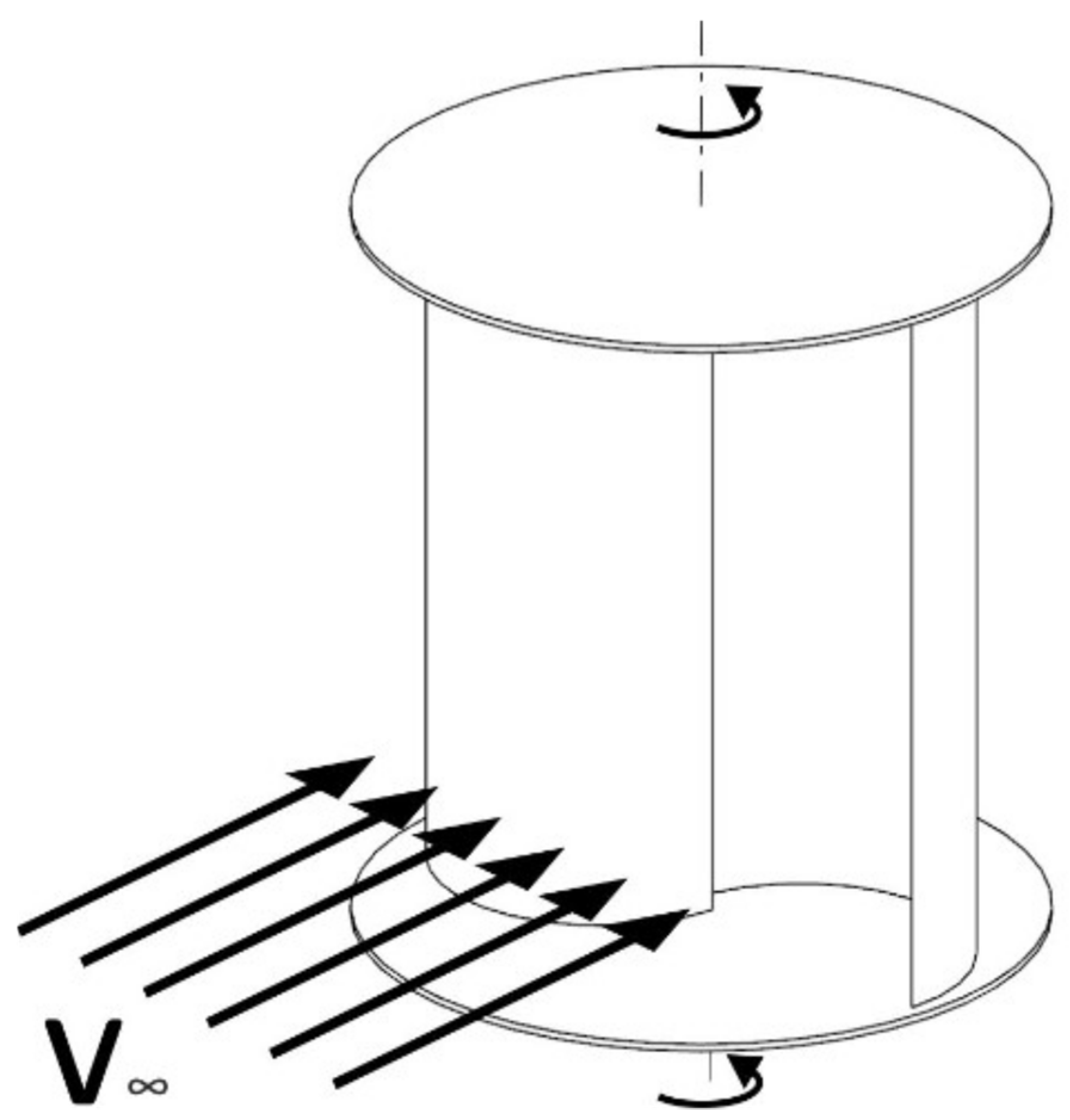
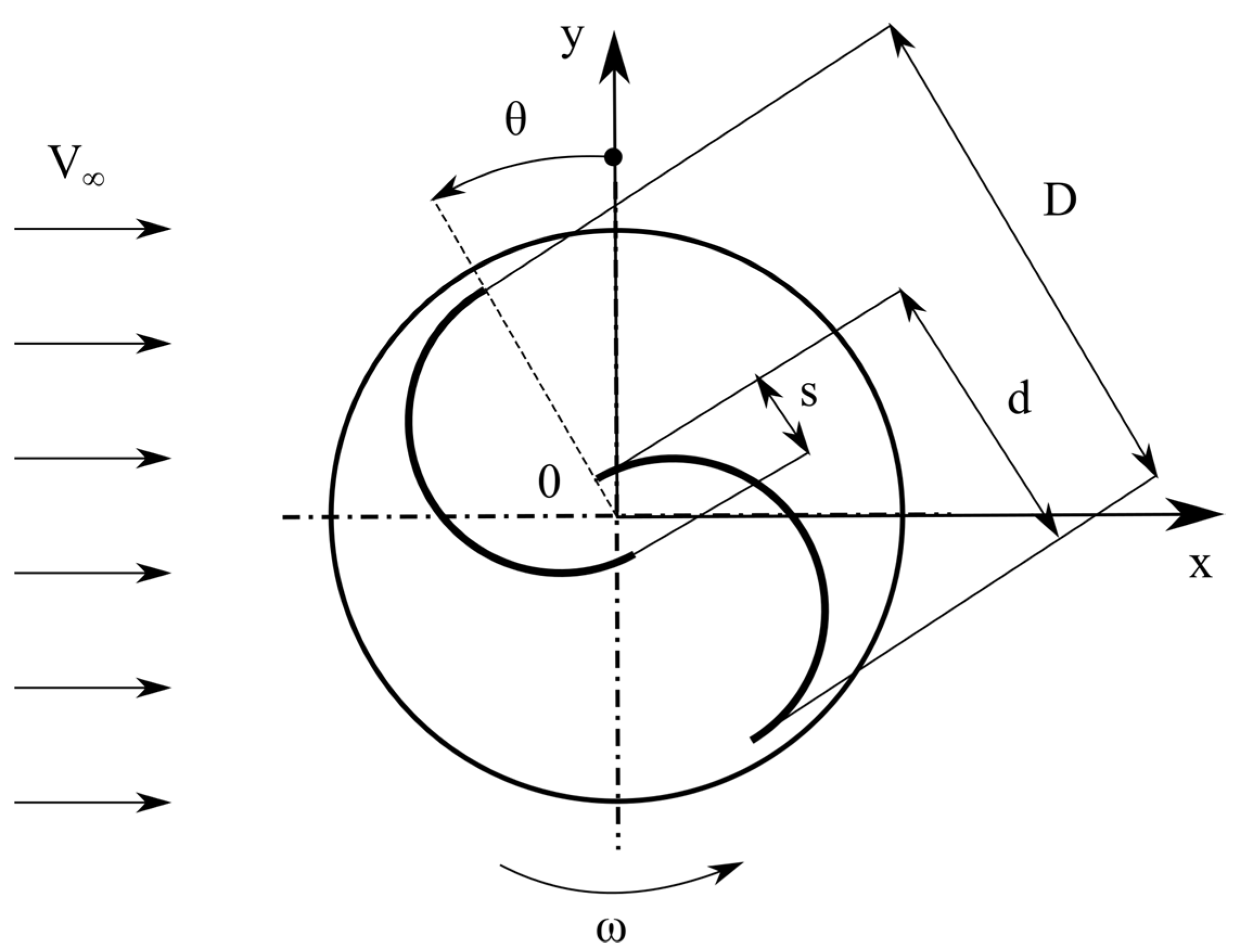
2.1. Description of the Rotor

Two-dimensional modeling for the geometry of the vertical-axis Savonius turbine in operation is performed in Figure 2. The rotor consists of two semicircular blades, whereas the dimensionless overlap ratio of this turbine, s/d, is equal to 0.10. The reason for choosing this overlap is the need to conduct a validation study based on the experimental results published in the report [10]. The dimensions of the vertical-axis Savonius turbine are given in Table 1.

2.2. Benchmark

In order to validate the CFD results, measurement data from the Sandia Laboratories report by Blackwell et al. were used [10,31]. The report by Blackwell et al. [10] is one of the older works on the aerodynamics of the Savonius wind turbine. However, the authors of this report put in a lot of effort to measure fifteen different rotor configurations in the wind tunnel. The aerodynamic performance of two- and three-bladed rotors was compared for different rotor heights, and different overlap ratios, for one- and two-stages and for two Reynolds numbers. The results of these measurements are a benchmark for many researchers [12,13,14,32,33,34,35,36,37]. Roy and Ducoin [16] compared the results of the average torque coefficient for three experiments by D’Alessandro et al. [38], Roy and Saha [39], and Blackwell et al. [10]. Although the experimental conditions for each reference were different, these compared characteristics are very similar. In the studies of Mereu et al. [27], C P and C Q coefficients were compared for 2D and 3D rotor models. It also turns out that the comparison of the results of numerical research using CFD methods with experimental results from different periods gives similar conclusions. That is, if the numerical model of the rotor is two-dimensional, then the obtained C P values are overestimated in comparison with these experiments [9].
Research by Blackwell et al. was carried out for two Reynolds numbers 4.32 × 10 5 and 8.67 × 10 5 . As this larger Reynolds number was much less often taken into account by researchers, all simulations presented in this paper have been performed for the larger Reynolds number. The Reynolds number is based on the rotor diameter and the bulk velocity:
R e = D · V ν
where ν is the kinematic viscosity of air. The validation process is based on dynamic experimental data [10].

2.3. Rotor Aerodynamic Performance

The torque, Q, generated by the rotor at a constant angular velocity, ω, cyclically varies during the rotation of the rotor. The rotor power, P, which is directly related to the torque, is used to evaluate the efficiency of the device. In order to calculate the aerodynamic efficiency of the device, called the power factor C P , the power, P, produced by the rotor should be divided by the power, Pavailable, available in the air stream flowing through the rotor cross-sectional area at the wind velocity V :
C P = P P a v a i l a b l e = Q ω ( 1 / 2 ) ρ A V 3 = C Q · T S R
where: A is the area of the rotor projected at the flow direction, C Q is the torque coefficient and T S R is the tip speed ratio. The last two values are defined, respectively, as follows:
C Q = Q ( 1 / 2 ) ρ A R V 2
T S R = ω R V
where R is the rotor radius. In this paper, the area A in Equations (2) and (3) is equal to:
A = ( 2 d s ) · H = ( 2 d s ) · 1 = 0.95   m 2
where: rotor high H in the present paper equals 1 m.

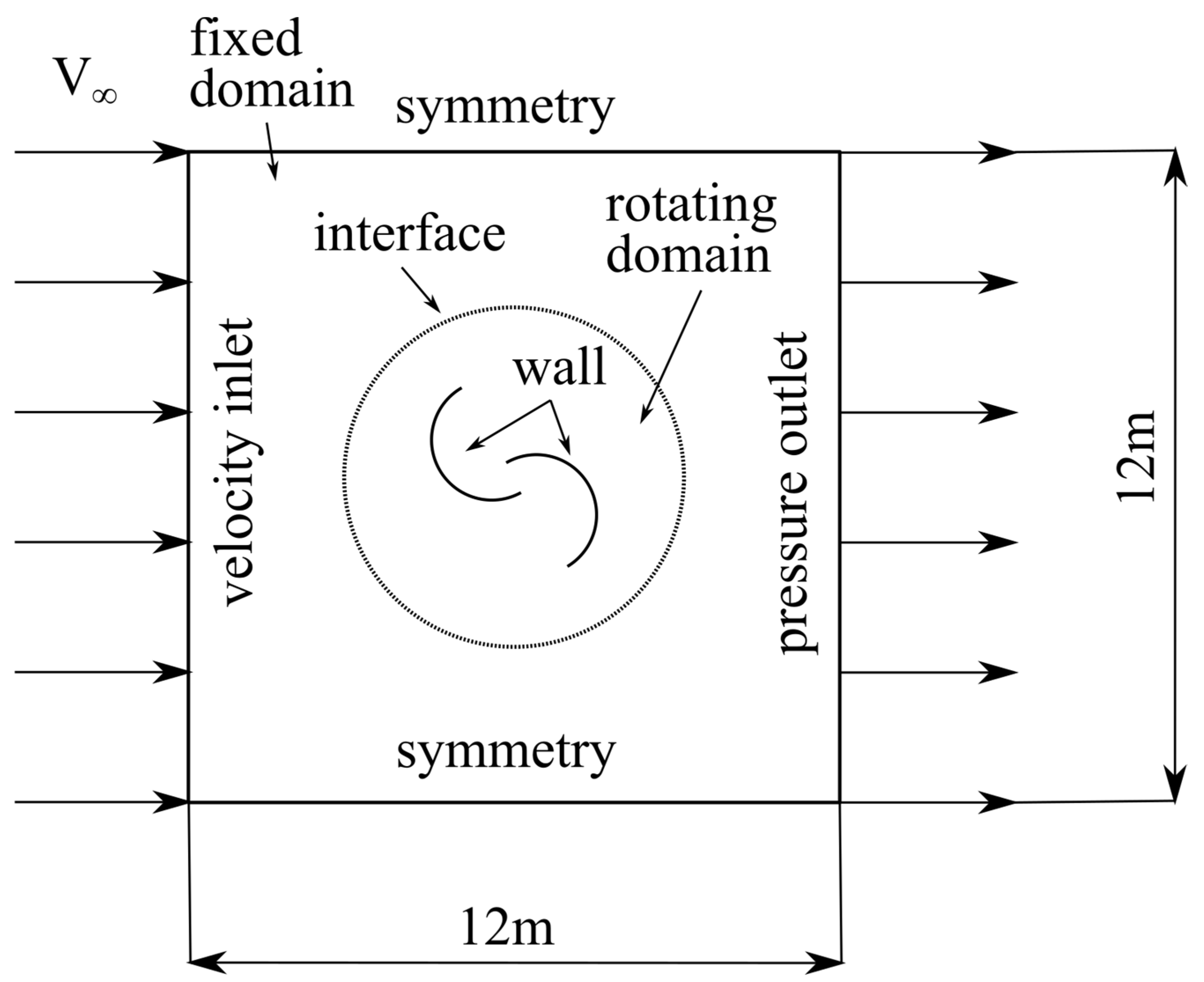
2.4. Computational Domain and Boundary Conditions

The computational domain consists of two parts: a rectangular fixed domain, and a circular rotating domain containing the wind turbine rotor, that rotates with the same angular velocity as the Savonius wind turbine. Too small a computational domain may affect the obtained aerodynamic characteristics. If the domain is not large enough and its boundaries are too close to the rotor, then air is artificially forced into the rotor because there is not enough room to flow around the turbine. This in turn causes an overestimation of the torque and aerodynamic efficiency of the device. Mohamed proved that the minimum distance from the rotor in each direction should be at least ten rotor diameters [40,41]. On this basis, in this study, a square computational domain, Figure 3, with a length of 12 m was selected for the simulation; therefore, the distance from the axis of rotation of the rotor to the boundaries of the domain is D/L = 12.63.
As shown in Figure 3, the velocity inlet boundary condition was assumed on the left vertical edge of the square domain, and on the right edge, the pressure outlet condition. On the other hand, the symmetry condition was defined on the upper and lower edges. The boundary condition “symmetry” can be employed to model zero-shear slip walls in viscous flows [42]. A circular sliding interface was used between the two parts of the domain, fixed and circular [11,12]. The distance between the rotor surfaces and the interface should be large enough that there are no errors in estimating distributions of vorticity [43,44]. To avoid numerical errors on the interface and their impact on the results of the velocity and pressure fields, the diameter of the circular part of the domain was set to 2 m. In Figure 4, the distributions of static pressure and velocity magnitude on the interfaces for the fixed and moving parts of the mesh are shown. This figure clearly shows that both the velocity and pressure profiles are the same on each mesh in the interface zone.

2.5. Solver Settings and Turbulence Model

For all 2D simulations presented in this paper, the time step size is equivalent to 1000 time steps per one complete revolution of the rotor, corresponding to 0.36° per time step. For unsteady Reynolds-averaged Navier-Stokes (URANS) simulations, the well-known SIMPLE algorithm was employed for pressure–velocity coupling. The gradients are computed employing the least-square cell-based method. All variables were calculated using second-order upwind schemes.
In this paper, the average fields of flow parameters in the rotor area are analyzed for three tip speed ratios: 0.75, 1.00, and 1.25. Each of these tip speed ratios corresponds to a different angular velocity of the rotor; the angular velocities for individual tip speed ratios are, respectively, equal to 22.10, 29.47, and 36.84 rad/s. For all the analyses shown in this paper, fifteen full rotations of the rotor were simulated in order to avoid the effect of initial conditions.
Popular CFD solvers such as ANSYS Fluent offer their users a wide choice of different turbulence models. The most popular and most frequently chosen models are the k-ε and k-ω models. These are, of course, the basic variants of these models. In applications with rotating blades and when using unstructured meshes, modified variants of these models are highly recommended, e.g., the realizable k-ε model or the SST k-ω model that blends both k-ε and k-ω turbulence models. The SST k-ω approach was used in this work due to its stability and high accuracy in solving the boundary layer [29]. The governing equations of these turbulence models are not presented in this paper because they are clearly described in the documentation of CFD solvers offering this turbulence model.

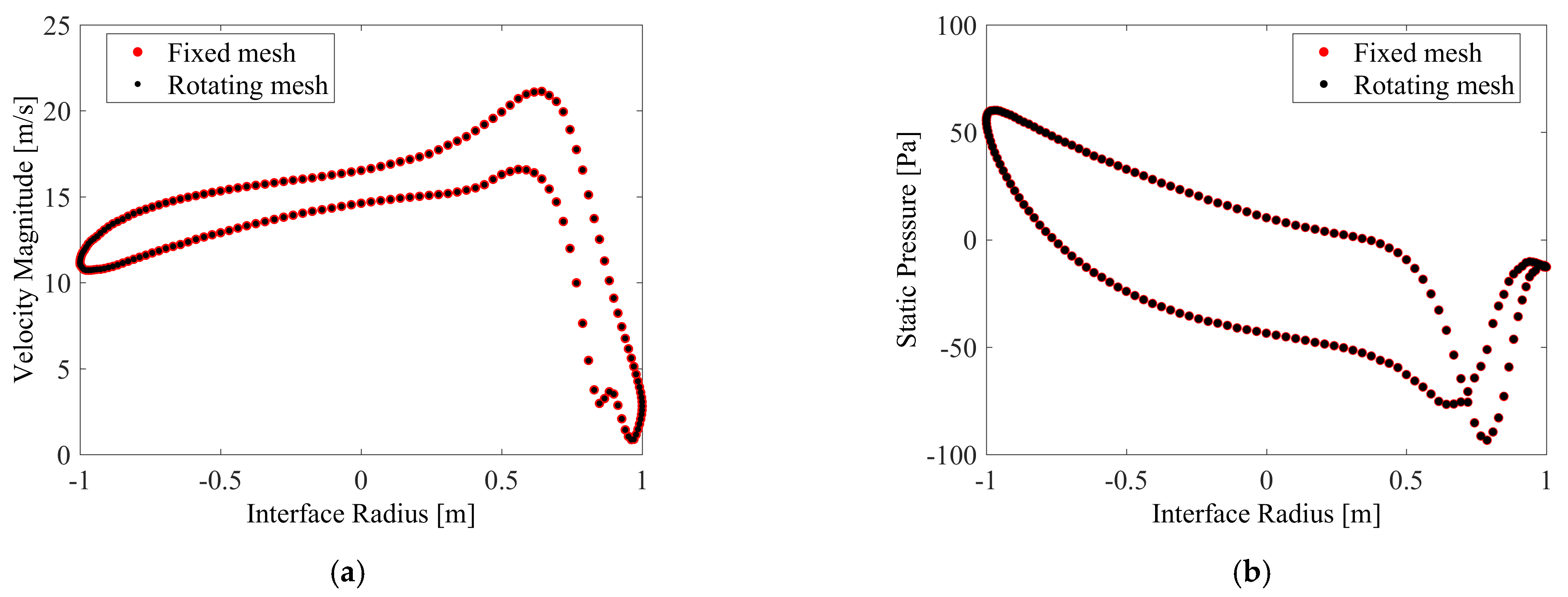
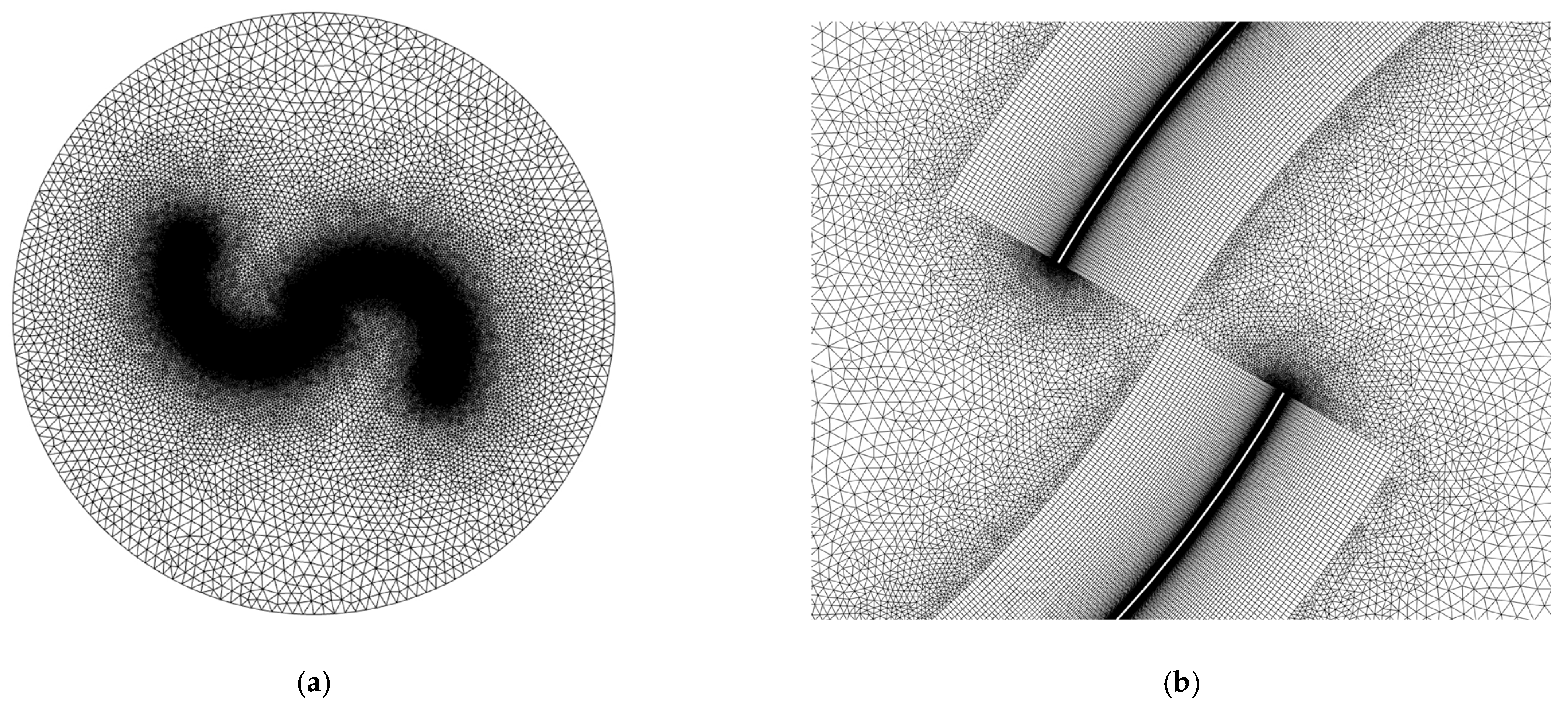
2.6. Mesh Convergence Study
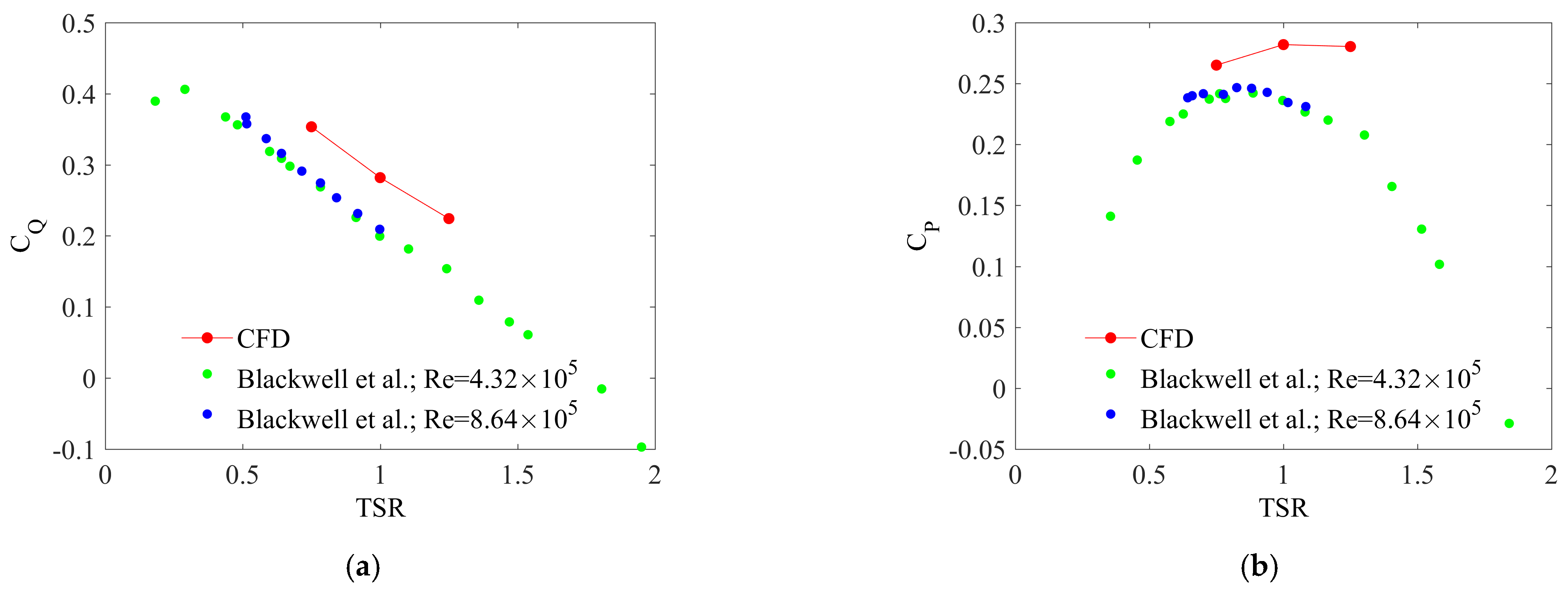
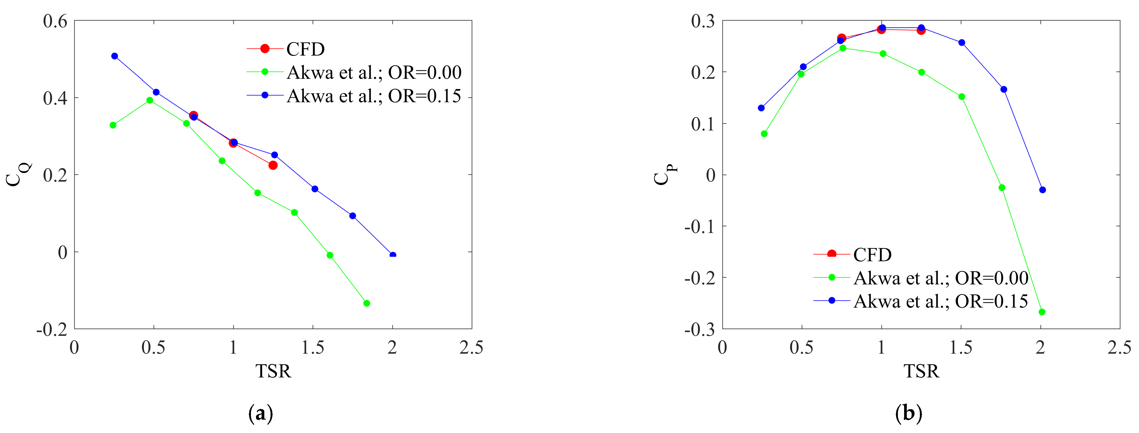
In order to determine an efficient mesh and to prevent divergence generated by an unsuitable mesh refinement strategy, a grid convergence study must be performed. In this paper, the computational domain was discretized using a hybrid mesh that consists of a quadrilateral structured mesh near the blades and a triangular unstructured mesh in the rest of the domain, as it is shown in Figure 5. The growth rate of the unstructured mesh was managed as 1.06; therefore, the grid density changed gradually, starting from the rotating domain. The structured part of the mesh was applied in order to capture the boundary layer viscous effects near the blades. The mesh first layer thickness from the blades was equal to 26 µm, which fulfills condition y+<1 required by turbulence models [40,45]. The number of structural mesh layers was 75, while the bias factor was 50. For a structured mesh, this bias factor corresponds to a growth rate of 1.06. We intended to provide a numerical grid that satisfies three assumptions at once: it will ensure small numerical dissipation of turbulence parameters between the inlet and the rotor; provides a smooth transition between structural and unstructured mesh elements; gives better numerical results of the wake behind the rotor. A grid independence study was performed for the three cases, as shown in Table 2. The three meshes used in the mesh sensitivity test differed in the number of nodes, N, on the edges of the rotor blades. The following three cases were investigated: N = 500, N = 750, and N = 1000. As can be seen from Table 2, the torque and power coefficients obtained for the coarse mesh are not significantly different from those for the fine mesh. Also, two publications proved that the number of nodes on the edges equal to 620 is sufficient for the solution to be independent of mesh density [46,47].

2.7. Validation

In these studies, the validation process was performed based on two data sources. The first source is the experiment [10] (Figure 6a,b), while the second is the numerical results from the publication [12] (Figure 7a,b). However, this second comparison is not direct because the results for a different value of the overlap ratio and a different value of the Reynolds number were compared. The second comparison makes sense, however, for two reasons. Firstly, Blackwell et al. [10] proved in their experiment that the differences in rotor aerodynamic performance are minimal for both Reynolds numbers 4.32 and 8.64. In Figure 6a,b, two sets of experimental data are summarized for these two Reynolds numbers. Second, the CFD results presented in this study were compared with two sets of numerical results by Akwa et al. [12]. These two datasets represent two overlap ratios of 0.0 and 0.15. These values are relatively close to those used in this study. As can be seen from Figure 6a,b, the nature of the numerical results is close to experimental. The obtained CFD values are also slightly different from the numerical results obtained by Akwa et al. [12], in particular, to those with an overlap ratio of 0.15.
Also, significant differences in the CFD (2D model) and experimental results were also observed by, among others, Talukdar et al. [9]. These authors concluded that the dimensionality effect excluded during the CFD simulations may be responsible for this minor discrimination. Ferrari et al. [14] conducted CFD studies of one of the Blackwell et al. [10] configurations (overlap ratio of 0.2 and R e = 4.32 · 10 5 ). Ferrari et al. [14] obtained similar accuracy of the numerical results for the 2D model compared to the experiment as the authors of this paper. Ferrari et al. proved that only the 3D model significantly improves the results.

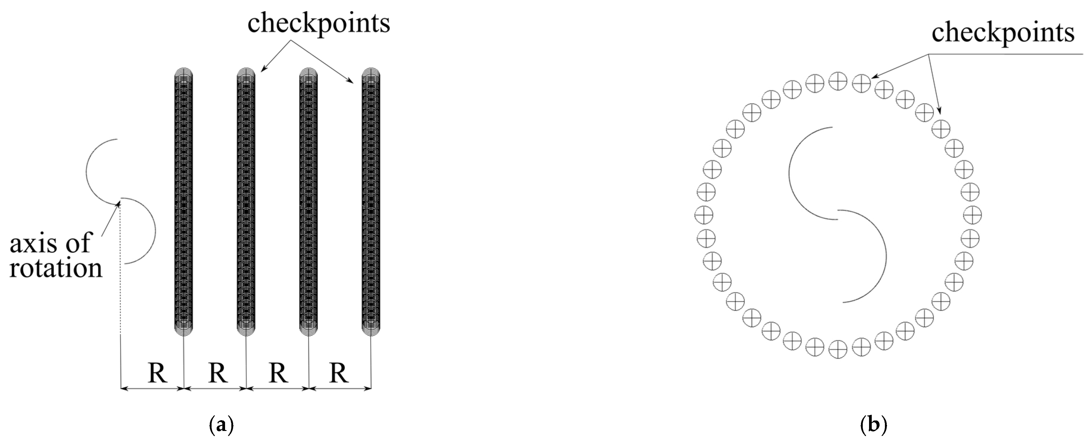
2.8. Flow Parameters Averaging Method

The primary purpose of this paper is to examine the averaged fields of flow parameters in the rotor area and the wake downstream behind the rotor, depending on the tip speed ratio. The averaged flow parameters analyzed in this work are two components of air velocity and static pressure. In order to study these values, two series of points were defined, where these instantaneous flow parameters were calculated, which were then saved to a file and then averaged. One series of checkpoints was typically arranged behind the rotor, as shown in Figure 8a. The second one was located around the rotor every 10 degrees at the distance D/2+d (according to the dimensions given in Table 1) from the axis of rotation of the rotor—Figure 8b. The sampling rate, f, was:
f = 18 · ω π

3. Results

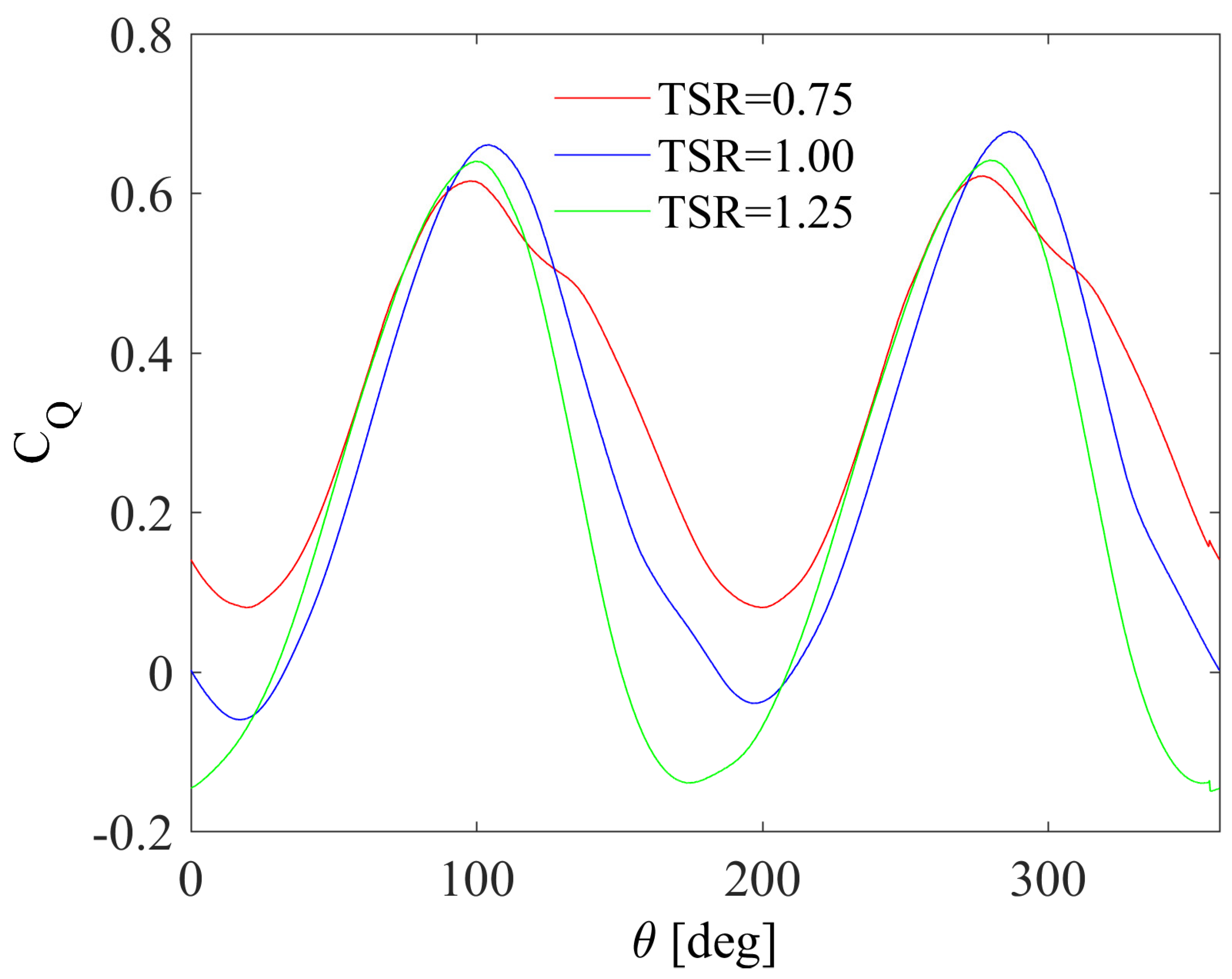
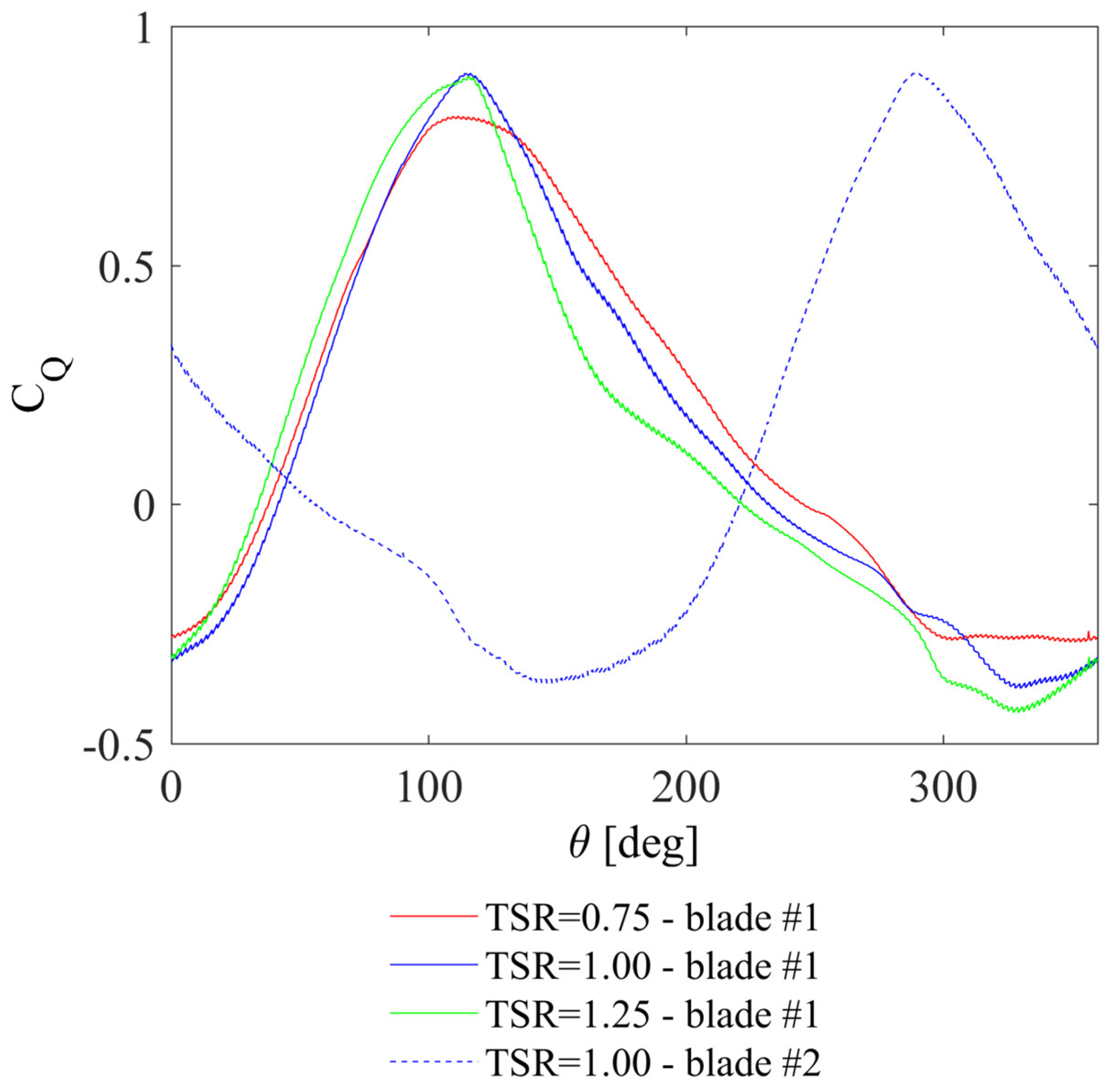
3.1. Torque Coefficient and Forces Acting on the Rotor

The dimensionless torque and power coefficients shown in Figure 6 and Figure 7 are, of course, the result of integrating the aerodynamic torque for one complete revolution of the rotor. Unlike conventional horizontal-axis wind turbines, the Savonius rotor’s aerodynamic moment significantly changes with azimuth. The lower the number of rotor blades, the larger the difference between the minimum and maximum torque. At the same time, the larger the number of rotor blades, the larger the number of torque changes per rotor revolution. Figure 9 shows the rotor aerodynamic moment as a dimensionless coefficient, according to Equation (3). The torque coefficient is also compared for three different values of the tip speed ratio. As can be seen in Figure 9, relatively small changes in the tip speed ratio provide significant differences in the amplitude of changes, i.e., in the difference between changes in the maximum and minimum value of the torque coefficient. The differences of these changes for TSR = 0.75, 1.00, and 1.25 are equal to 5, 10, and 15 respectively. It is also worth noting that at a constant angular velocity, the changes in the power coefficient for the first and second halves of the rotation are the same. Moreover, as can be seen in Figure 9, the maximum values of the torque coefficient are the highest for the optimal tip speed ratio. On the other hand, the modules of the minimum values of this coefficient increase with the increase of the tip speed ratio. It is also clear that the tip speed ratio significantly affects these lower values of the torque coefficient. The last thing worth observing is the faster occurrence of the minimum values of the torque coefficient for higher and higher tip speed ratios.
In addition to the total torque acting on the entire rotor (Figure 9), it is also interesting how the individual blades contribute to this torque. Figure 10 compares the torque characteristics for one blade for three tip speed ratios. In addition, for TSR = 1.0, the torque characteristics were compared separately for the first and second blades. As it turns out, the torque characteristics for each of the blades are not as different from each other as the total torque acting on the rotor. The maximum values of the torque coefficient for the two largest tip speed ratios investigated in this work reach almost the same value. The largest differences between the three curves are visible in the results for the downstream part of the rotor. The most important observation, however, is that each blade produces a positive torque in the azimuth range from 34–38 to 222–245 degrees, depending on the tip speed ratio. That means, as the tip speed increases, the aerodynamic drag acting on the blade in the downstream part of the rotor increases.

3.2. Averaged Flow Parameters

Figure 11 and Figure 12 show the average flow parameters around the rotor. Figure 11a,b shows the two components of the flow velocity, a component, Vx, parallel to the wind direction, and a component, Vy, perpendicular, respectively. In contrast, Figure 12a,b shows the flow angle and the static pressure distribution around the rotor, respectively. The velocities in Figure 11 have been normalized by the undisturbed flow velocity V . This flow angle is defined as t a n   1 ( V y / V x ) [48] and expressed in degrees. All results are compared for three tip speed ratios.
Analyzing the distribution of the Vx component of the flow velocity (Figure 11a), two characteristic decreases in this velocity can be seen. The first is for the windward part of the rotor, for azimuth in the range of 0 to 180 degrees, and the second is for the leeward part, for azimuth in the range of 180 to 360 degrees. Of course, the velocity drop in this second part of the rotor is greater compared to the velocity drop in the windward part. What is evident from these results, however, is that the velocity distribution is not significantly TSR-dependent. The average velocity for all tip speed ratios for the windward part of the rotor is 12.49 m/s and for the leeward part, it is equal to 8.79 m/s. It is worth emphasizing that with increasing tip speed ratio, average Vx decrease, but these differences are negligible. The difference in average velocity Vx for TSR = 0.75 and 1.25 is 0.08 m/s for the windward part and 0.48 for the leeward part. This is therefore a difference of less than one meter per second. This is a different tendency than in the case of the Darrieus wind turbine, for which the distribution of the average velocity Vx depends quite significantly on the tip speed ratio [49,50]. In addition, unlike the Darrieus wind turbine, a significant increase in the average velocity Vx can be seen near the azimuth of 180 degrees. In the case of the Darrieus wind turbine, for this azimuth and for optimal TSR, it can be seen that the local flow velocity Vx reaches or slightly exceeds the wind velocity V [50]. In contrast, in the case of the Savonius wind turbine, the local velocity Vx can increase by up to 32% on average compared to the undisturbed flow velocity V . It is also interesting that the maximum value of this velocity is localized for the azimuth of 190–200 degrees. Thus, it appears already in the downwind part of the rotor. On the other hand, the area for which the velocity ratio V x / V is greater than one and extends in the azimuth range from 140 to 220 degrees. This local increase in the average speed Vx up to the azimuth of about 200 degrees entails a decrease in the rotor torque coefficient (Figure 9), which for the azimuth of 172–200 degrees, depending on the tip speed ratio, reaches a minimum value.
In the downwind part of the rotor, a significant decrease in Vx velocity down to a negative value is visible, which means that locally, the flow velocity is opposite to the direction of the wind (In the leeward part of the rotor, a significant decrease in Vx velocity down to a negative value is visible, which means that locally the flow velocity is opposite to the direction of the wind). This local velocity Vx drop also significantly modifies the velocity component field Vy (Figure 11b), and the static pressure field (Figure 12b). The minimum value of the velocity Vx was obtained with an average of −0.73 m/s, which corresponds to an azimuth of 300 degrees and a maximum flow angle of 122 degrees on average (Figure 11b).
The pressure reaches a local minimum value at the azimuth of 220 degrees, which is shown in Figure 12a. At this azimuth, both blades simultaneously achieve a very similar torque value close to zero, which can be seen in Figure 10. This pressure peak seen in the graph is also directly related to the presence of a vortex structure that is formed at the tip of the blade from an azimuth of about 136 degrees (Figure 13).
Figure 14, Figure 15 and Figure 16 illustrate the distribution of pressure and velocity components in the wake downstream behind the rotor. These results shown in the graphs were calculated on defined rakes located behind the rotor as shown in Figure 8. The instantaneous values were then averaged, as discussed in Section 2.8 of this paper. In contrast to the velocity distributions, the characteristics of the pressures behind the rotor differ significantly more depending on the tip speed ratio. Therefore, in Figure 14 and Figure 15, these relationships are shown separately for each of the rakes. It is clear from these graphs that these results are a function of both the tip speed ratio and the x and y coordinates. The largest pressure drop is visible for the location x/R = 1 and the case TSR = 0.75. However, this research has shown that the greatest impact on the velocity distribution, especially the component parallel to the direction of undisturbed flow, has the distance from the rotor axis. Therefore, in order to save space, only the results for the case TSR = 1.00 are presented in this article in Figure 16. These studies have shown that as the x coordinate increases, the velocity distribution Vx becomes more and more symmetric concerning the y = 0 coordinate. This is due to the weakening of the vortex flowing down from the lower blade.

4. Conclusions

In this paper, the average values of static pressure and velocity components around the rotor were studied. The purpose of this analysis is to examine the effect of the tip speed ratio on the average velocity field and the pressure field around the rotor and to compare the flow parameters for two rotor halves: windward and leeward. Based on the conducted research, the following conclusions were obtained:
  • Aerodynamic performance, rotor power coefficient, directly depends on aerodynamic torque. The aerodynamic torque of the two-bladed rotor changes significantly with azimuth. The operation of the rotor at these tip speed ratios requires, of course, the use of a second additional rotor section with blades rotated 90 degrees relative to the first section;
  • Each blade produces a positive torque in the azimuth range from 34–38 to 222–245 degrees, depending on the tip speed ratio. As the tip speed increases, the aerodynamic drag acting on the blade in the downstream part of the rotor increases;
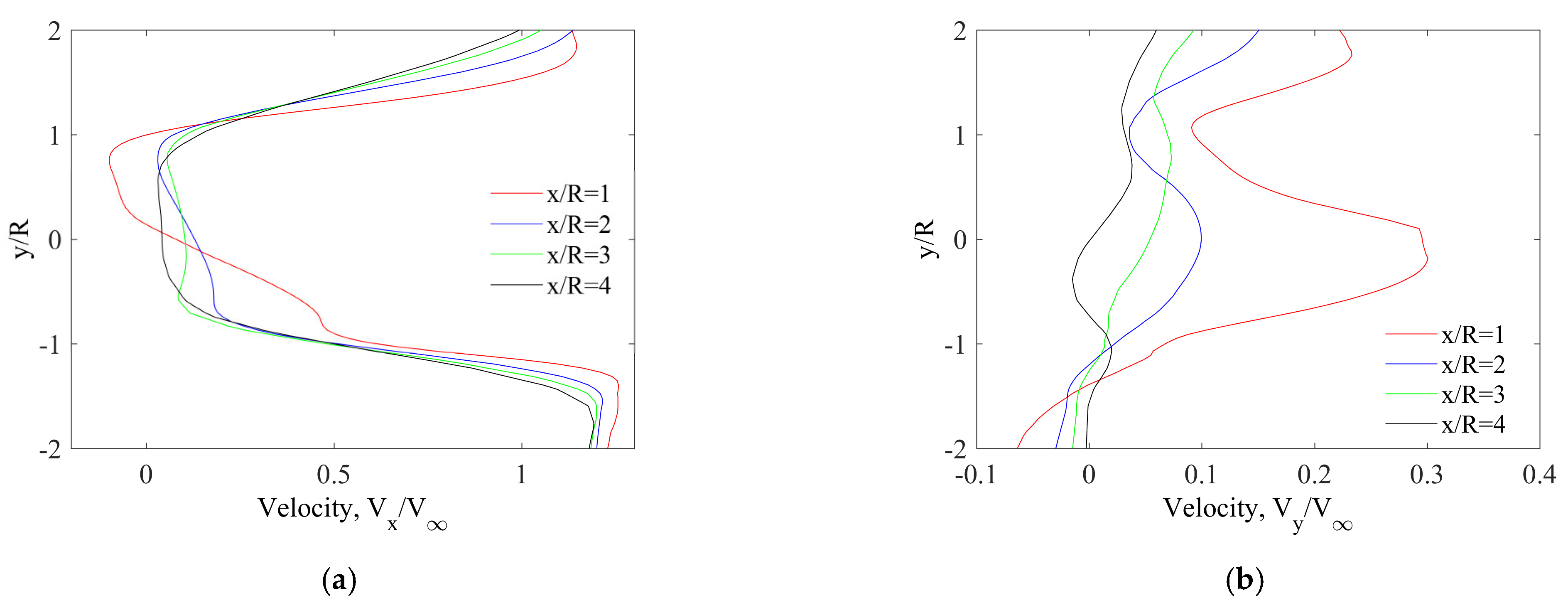
  • Contrary to the Darrieus rotor, in the case of the Savonius rotor, the tip speed ratio has little influence on the average speed distribution around the rotor. This applies to both the velocity component parallel to the direction of undisturbed flow and the perpendicular component. In the upwind part of the rotor, the average velocity parallel to the direction of undisturbed flow is on average 29% lower than in the downwind part;
  • In the case of the Savonius wind turbine, an increase in the Vx velocity can be observed locally in relation to the undisturbed flow velocity. Locally, the velocity component Vx may be as much as 32% higher when compared to the velocity V. In addition, the maximum of the velocity component Vx is observed already in the leeward part of the rotor;
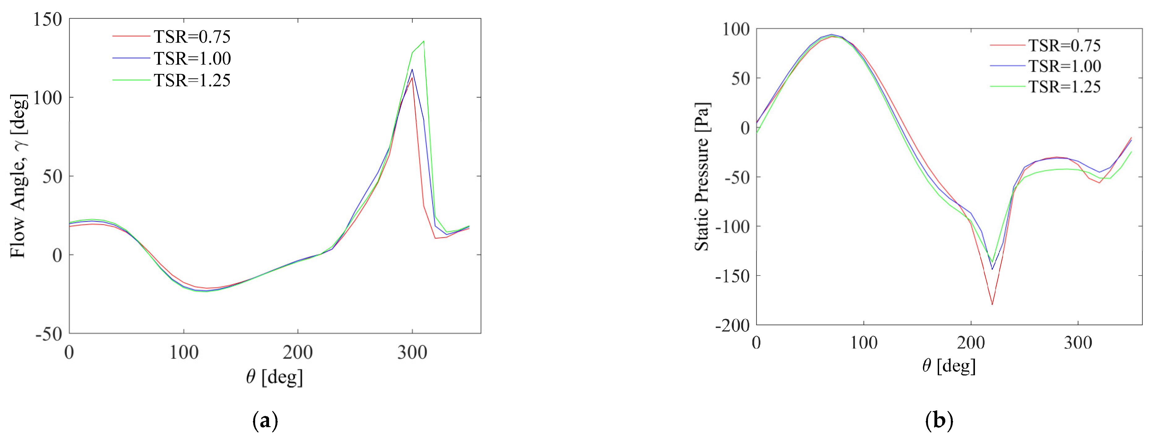
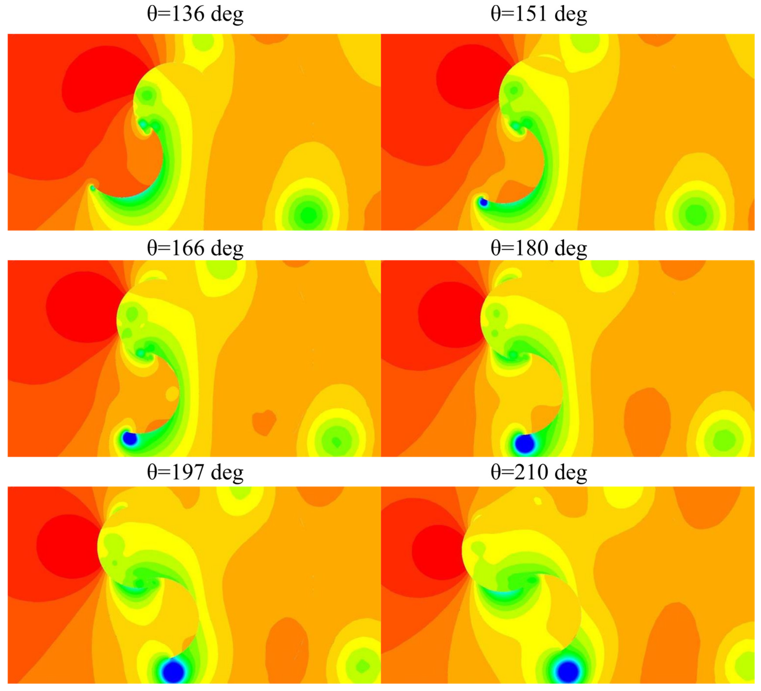
  • In the downwind part of the rotor, the flow is much more complex. Both the pressure and the flow angle reach their extreme values. On the other hand, the velocity component Vx reaches a locally negative value. This is directly influenced by the geometry of the rotor and the aerodynamic performance of the rotor blades;
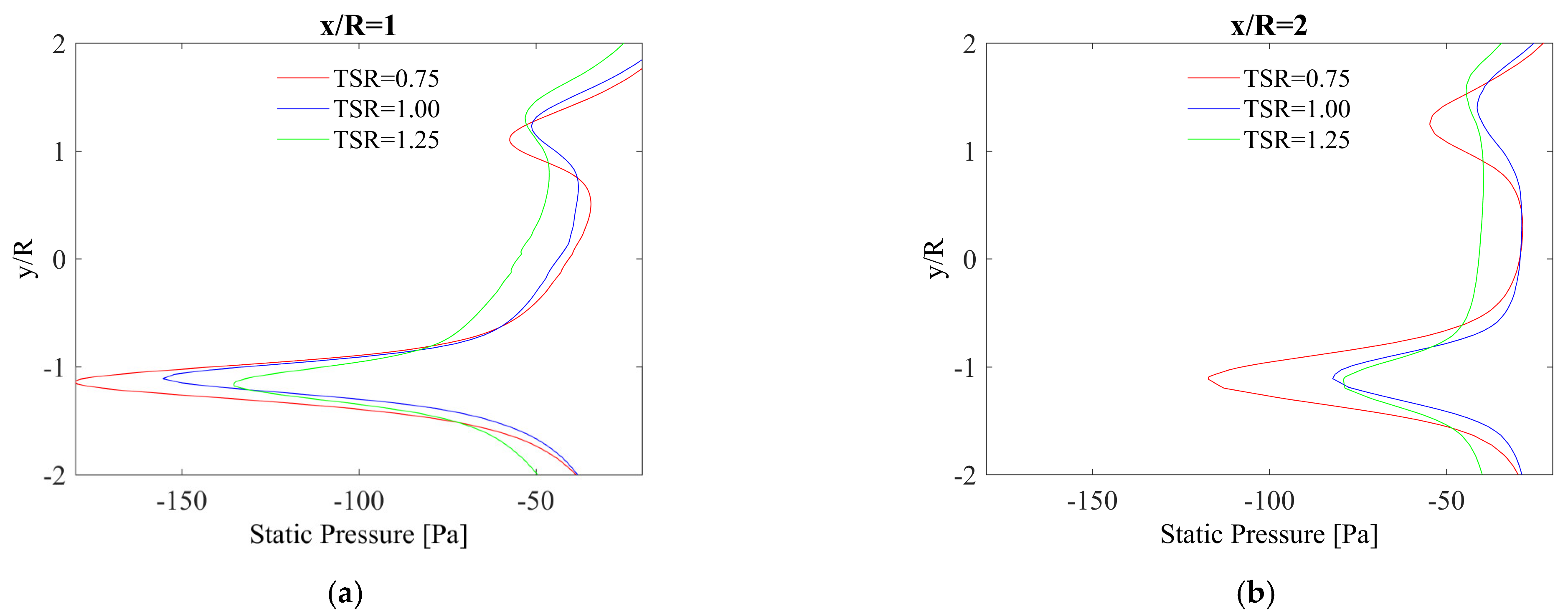
  • Negative static pressure is visible throughout the area on the downwind part of the rotor. This is another significant difference compared to Darrieus wind turbine rotor with high solidity and operating at low tip speed ratios [49];
  • The influence of the tip speed ratio on the pressure distribution in the wake downstream behind the rotor is much larger than in the case of the pressure distribution around the rotor;
  • As in the case of the distribution of velocity components around the rotor, the impact of the tip speed ratio on the velocity distributions in wake is definitely much smaller;
  • Both the static pressure and the tip speed ratio are a function of the distance from the axis of the rotor;
  • As the distance from the rotor axis increases, the velocity Vx distribution becomes more symmetrical with respect to the y = 0 coordinate; and
  • Moving away from the rotor axis has a much greater effect on the pressure distribution than on the velocity distribution.

Author Contributions

Conceptualization, J.M. and K.R.; methodology, J.M. and K.R.; software, J.M. and K.R.; validation, J.M.; formal analysis, J.M. and K.R.; investigation, J.M. and K.R.; data curation, J.M. and K.R.; writing—original draft preparation, K.R.; writing—review and editing, J.M.; visualization, J.M. and K.R.; supervision, K.R.; project administration, K.R.; funding acquisition, K.R. All authors have read and agreed to the published version of the manuscript.

Funding

Research was funded by POB Energy of Warsaw University of Technology within the Excellence Initiative: Research University (IDUB) programme (Grant No. 1820/355/Z01/POB7/2021). This research was supported in part by PL-Grid Infrastructure.

Institutional Review Board Statement

Not applicable.

Informed Consent Statement

Not applicable.

Data Availability Statement

The data presented in this study are available upon request from the corresponding author.

Acknowledgments

The authors would like to thank the editors and reviewers for their valuable comments on this research.

Conflicts of Interest

The authors declare no conflict of interest.

References

  1. Yao, J.; Li, F.; Chen, J.; Yuan, Z.; Mai, W. Parameter Analysis of Savonius Hydraulic Turbine Considering the Effect of Reducing Flow Velocity. Energies 2020, 13, 24. [Google Scholar] [CrossRef] [Green Version]
  2. Savonius, S. The S-Roter and Its Applications. Mech. Eng. 1931, 53, 333–338. [Google Scholar]
  3. Sivasegaram, S. Design parameters affecting the performance of resistance-type, vertical-axis windrotors—An experimental investigation. Wind Energy 1977, 1, 207–217. [Google Scholar]
  4. Shigetomi, A.; Murai, Y.; Tasaka, Y.; Tasaka, Y. Interactive flow field around two Savonius turbines. Renew. Energy 2011, 36, 536–545. [Google Scholar] [CrossRef]
  5. Pope, K.; Dincer, I.; Naterer, G. Energy and energy efficiency comparison of horizontal and vertical axis wind turbines. Renew. Energy 2010, 35, 2102–2113. [Google Scholar] [CrossRef]
  6. Tian, W.; Song, B.; Van Zwieten, J.H.; Pyakurel, P. Computational Fluid Dynamics Prediction of a Modified Savonius Wind Turbine with Novel Blade Shapes. Energies 2015, 8, 7915–7929. [Google Scholar] [CrossRef] [Green Version]
  7. Menet, J.-L. A double-step Savonius rotor for local production of electricity: A design study. Renew. Energy 2004, 29, 1843–1862. [Google Scholar] [CrossRef]
  8. Olabi, A.G.; Wilberforce, T.; Elsaid, K.; Salameh, T.; Sayed, E.T.; Husain, K.S.; Abdelkareem, M.A. Selection Guidelines for Wind Energy Technologies. Energies 2021, 14, 3244. [Google Scholar] [CrossRef]
  9. Talukdar, P.K.; Sardar, A.; Kulkarni, V.; Saha, U.K. Parametric analysis of model Savonius hydrokinetic turbines through experimental and computational investigations. Energy Convers. Manag. 2018, 158, 36–49. [Google Scholar] [CrossRef]
  10. Blackwell, B.; Sheldahl, R.; Feltz, L. Wind Tunnel Performance Data for Two-and-Three-Bucket Savonius Rotors; US Sandia Laboratories Report SAND76-0131; Sandia Laboratories: Springfield, VA, USA, 1977. [Google Scholar]
  11. Nakajima, M.; Iio, S.; Ikeda, T. Performance of double-step Savonius rotor for environmentally friendly hydraulic turbine. J. Fluid Sci. Tech. 2008, 3, 410–419. [Google Scholar] [CrossRef] [Green Version]
  12. Akwa, J.; Junior, G.; Petry, A. Discussion on the verification of the overlap ratio influence on performance coefficients of a Savonius wind rotor using computational fluid dynamics. Renew. Energy 2012, 38, 141–149. [Google Scholar] [CrossRef]
  13. Meziane, M.; Faqir, M.; Essadiqi, E.; Ghanameh, M.F. CFD analysis of the effects of multiple semicircular blades on Savonius wind turbine performance. Int. J. Renew. Energy Res. 2020, 10, 1316–1326. [Google Scholar] [CrossRef]
  14. Ferrari, G.; Federici, D.; Schito, P.; Inzoli, F.; Mereu, R. CFD study of Savonius wind turbine: 3D model validation and parametric analysis. Renew. Energy 2017, 105, 722–734. [Google Scholar] [CrossRef]
  15. Zhou, T.; Rempfer, D. Numerical study of detailed flow field and performance of Savonius wind turbines. Renew. Energy 2013, 51, 373–381. [Google Scholar] [CrossRef]
  16. Roy, S.; Ducoin, A. Unsteady analysis on the instantaneous forces and moment arms acting on a novel Savonius-style wind turbine. Energy Convers. Manag. 2016, 121, 281–296. [Google Scholar] [CrossRef]
  17. Fernando, M.S.U.K.; Modi, V. A numerical analysis of the unsteady flow past a Savonius wind turbine. J. Wind Eng. Ind. Aerodyn. 1989, 32, 302–327. [Google Scholar] [CrossRef]
  18. Mendoza, V.; Katsidoniotaki, E.; Bernhoff, H. Numerical Study of a Novel Concept for Manufacturing SAVONIUS Turbines with Twisted Blades. Energies 2020, 13, 1874. [Google Scholar] [CrossRef] [Green Version]
  19. Marinić-Kragić, I.; Vučina, D.; Milas, Z. Global optimization of Savonius-type vertical axis wind turbine with multiple circular-arc blades using validated 3D CFD model. Energy 2022, 241, 122841. [Google Scholar] [CrossRef]
  20. Nasef, M.H.; El-Askary, W.A.; AbdEL-hamid, A.A.; Gad, H.E. Evaluation of Savonius rotor performance: Static and dynamic studies. J. Wind Eng. Ind. Aerodyn. 2013, 123, 1–11. [Google Scholar] [CrossRef]
  21. Aboujaoude, H.; Beaumont, F.; Murer, S.; Polidori, G.; Bogard, F. Aerodynamic performance enhancement of a Savonius wind turbine using an axisymmetric deflector. J. Wind. Eng. Ind. Aerodyn. 2022, 220, 104882. [Google Scholar] [CrossRef]
  22. Elbatran, A.H.; Elbatran, Y.M.; Shehata, A.S. Shehata. Performance study of ducted nozzle Savonius water turbine, comparison with conventional Savonius turbine. Energy 2017, 134, 566–584. [Google Scholar] [CrossRef]
  23. El-Askary, W.A.; Nasef, M.H.; Abdel-Hamid, A.A.; Gad, H.E. Harvesting wind energy for improving performance of Savonius rotor. J. Wind Eng. Ind. Aerodyn. 2015, 139, 8–15. [Google Scholar] [CrossRef]
  24. Ramarajan, J.; Jayavel, S. Numerical study on the effect of out-of-phase wavy confining walls on the performance of Savonius rotor. J. Wind Eng. Ind. Aerodyn. 2022, 226, 105023. [Google Scholar] [CrossRef]
  25. Longo, R.; Nicastro, P.; Natalini, M.; Schito, P.; Mereu, R.; Parente, A. Impact of urban environment on Savonius wind turbine performance: A numerical perspective. Renew. Energy 2020, 156, 407–422. [Google Scholar] [CrossRef]
  26. Shaheen, M.; El-Sayed, M.; Abdallah, S. Numerical study of two-bucket Savonius wind turbine cluster. J. Wind Eng. Ind. Aerod 2015, 137, 78–89. [Google Scholar] [CrossRef]
  27. Mereu, R.; Federici, D.; Ferrari, G.; Schito, P.; Inzoli, F. Parametric numerical study of Savonius wind turbine interaction in a linear array. Renew. Energy 2017, 113, 1320–1332. [Google Scholar] [CrossRef]
  28. Rogowski, K.; Maroński, R. CFD computation of the Savonius rotor. J. Theor. Appl. Mech. 2015, 53, 37–45. [Google Scholar] [CrossRef] [Green Version]
  29. Larin, P.; Paraschivoiu, M.; Aygun, C. CFD based synergistic analysis of wind turbines for roof mounted integration. J. Wind Eng. Ind. Aerodyn. 2016, 156, 1–13. [Google Scholar] [CrossRef]
  30. Mao, Z.; Yang, G.; Zhang, T.; Tian, W. Aerodynamic Performance Analysis of a Building-Integrated Savonius Turbine. Energies 2020, 13, 2636. [Google Scholar] [CrossRef]
  31. Sheldahl, R.E.; Feltz, L.V.; Blackwell, B.F. Wind tunnel performance data for two-and three-bucket Savonius rotors. J. Energy 1978, 2, 160–164. [Google Scholar] [CrossRef] [Green Version]
  32. Zhang, B.; Song, B.; Mao, Z.; Tian, W.; Li, B.; Li, B. A Novel Parametric Modeling Method and Optimal Design for Savonius Wind Turbines. Energies 2017, 10, 301. [Google Scholar] [CrossRef] [Green Version]
  33. Sun, X.; Luo, D.; Huang, D.; Wu, G. Numerical study on coupling effects among multiple Savonius turbines. J. Renew. Sustain. Energy 2012, 4, 053107. [Google Scholar] [CrossRef]
  34. Alaimo, A.; Esposito, A.; Milazzo, A.; Orlando, C.; Trentacosti, F. Slotted Blades Savonius Wind Turbine Analysis by CFD. Energies 2013, 6, 6335–6351. [Google Scholar] [CrossRef]
  35. Kim, S.; Cheong, C. Development of low-noise drag-type vertical wind turbines. Renew. Energy 2015, 79, 199–208. [Google Scholar] [CrossRef]
  36. Blanco Damota, J.; Rodríguez García, J.d.D.; Couce Casanova, A.; Telmo Miranda, J.; Caccia, C.G.; Galdo, M.I.L. Optimization of a Nature-Inspired Shape for a Vertical Axis Wind Turbine through a Numerical Model and an Artificial Neural Network. Appl. Sci. 2022, 12, 8037. [Google Scholar] [CrossRef]
  37. dos Santos, A.L.; Fragassa, C.; Santos, A.L.G.; Vieira, R.S.; Rocha, L.A.O.; Conde, J.M.P.; Isoldi, L.A.; dos Santos, E.D. Development of a Computational Model for Investigation of and Oscillating Water Column Device with a Savonius Turbine. J. Mar. Sci. Eng. 2022, 10, 79. [Google Scholar] [CrossRef]
  38. Alessandro, D.; Montelpare, S.; Ricci, R.; Secchiaroli, A. Unsteady Aerodynamics of a Savonius wind rotor: A new computational approach for the simulation of energy performance. Energy 2010, 35, 3349–3363. [Google Scholar] [CrossRef]
  39. Roy, S.; Saha, U.K. Wind tunnel experiments of a newly developed two-bladed Savonius-style wind turbine. Appl. Energy 2015, 137, 117–125. [Google Scholar] [CrossRef]
  40. Mohamed, M.H.; Thevenin, D. Performance optimization of a Savonius turbine considering different shapes for frontal guiding plates. In Proceedings of the 10th International Conference of Fluid Dynamics ICFD, Cairo, Egypt, 16–19 December 2010. [Google Scholar]
  41. Mohamed, M.H.; Janiga, G.; Pap, E.; Thévenin, D. Optimal blade shape of a modified Savonius turbine using an obstacle shielding the returning blade. Energy Convers. Manag. 2011, 52, 236–242. [Google Scholar] [CrossRef]
  42. ANSYS, Inc. ANSYS Fluent Theory Guide, Release 19.1.; ANSYS, Inc.: Canonsburg, PA, USA, 2019. [Google Scholar]
  43. Bangga, G.; Hutomo, G.; Wiranegara, R.; Sasongko, H. Numerical study on a single bladed vertical axis wind turbine under dynamic stall. J. Mech. Sci. Technol. 2017, 31, 261–267. [Google Scholar] [CrossRef]
  44. Rogowski, K. Numerical studies on two turbulence models and a laminar model for aerodynamics of a vertical-axis wind turbine. J. Mech. Sci. Technol. 2018, 32, 2079–2088. [Google Scholar] [CrossRef]
  45. Kacprzak, K.; Liskiewicz, G.; Sobczak, K. Numerical investigation of conventional and modified Savonius wind turbines. Renew. Energy 2013, 60, 578–585. [Google Scholar] [CrossRef]
  46. Bouzaher, M.T.; Guerira, B. Impact of Flexible Blades on the Performance of Savonius Wind Turbine. Arab J. Sci. Eng. 2022, 47, 15365–15377. [Google Scholar] [CrossRef]
  47. Mari, M.; Venturini, M.; Beyene, A. Performance Evaluation of Novel Spline-Curved Blades of a Vertical Axis Wind Turbine Based on the Savonius Concept. In Proceedings of the ASME 2016 International Mechanical Engineering Congress and Exposition, Phoenix, AZ, USA, 11–17 November 2016. [Google Scholar] [CrossRef]
  48. Hansen, M.O.L. Aerodynamics of Wind Turbines; Earthscan: London, UK, 2008. [Google Scholar]
  49. Rogowski, K.; Maroński, R.; Piechna, J. Numerical analysis of a small-size vertical-axis wind turbine performance and averaged flow parameters around the rotor. Arch. Mech. Eng. 2017, 64, 205–218. [Google Scholar] [CrossRef]
  50. Madsen, H.; Larsen, T.; Vita, L.; Paulsen, U. Implementation of the Actuator Cylinder flow model in the HAWC2 code for aeroelastic simulations on Vertical Axis Wind Turbines. In Proceedings of the 51st AIAA Aerospace Sciences Meeting Including the New Horizons Forum and Aerospace Exposition, Grapevine, TX, USA, 7–10 January 2013. [Google Scholar] [CrossRef]
Figure 1. Silhouette of the Savonius wind turbine.
Energies 16 00281 g001
Figure 2. Conventional two-bladed Savonius wind turbine.
Energies 16 00281 g002
Figure 3. Computational domain and boundary conditions.
Energies 16 00281 g003
Figure 4. Flow parameters across the two sides of the interface zone: (a) Velocity profiles; (b) static pressure profiles.
Energies 16 00281 g004
Figure 5. 2D mesh for two-bladed rotor: (a) Mesh of the rotating domain; (b) the zoom view on mesh details around the blade.
Energies 16 00281 g005
Figure 6. Comparison of CFD results with the experiment [10]: (a) Torque coefficient; (b) power coefficient.
Energies 16 00281 g006
Figure 7. Comparison of CFD results with numerical results from [12]: (a) Torque coefficient; (b) power coefficient.
Energies 16 00281 g007
Figure 8. Checkpoints for recording speeds and pressures: (a) Points in the wake; (b) points around the rotor.
Energies 16 00281 g008
Figure 9. Torque coefficient as a function of azimuth.
Energies 16 00281 g009
Figure 10. Torque coefficient acting on individual blades.
Energies 16 00281 g010
Figure 11. Average flow parameters around the rotor: (a) Vx velocity component; (b) Vy velocity component.
Energies 16 00281 g011
Figure 12. Average flow parameters around the rotor: (a) Flow angle; (b) static pressure.
Energies 16 00281 g012
Figure 13. Instantaneous static pressure distributions for the tip speed ratio of 1.00.
Energies 16 00281 g013
Figure 14. Static pressure in the wake: (a) Location x/R = 1 behind the rotor axis; (b) location x/R = 2 behind the rotor axis.
Energies 16 00281 g014
Figure 15. Static pressure in the wake: (a) Location x/R = 3 behind the rotor axis; (b) location x/R = 4 behind the rotor axis.
Energies 16 00281 g015
Figure 16. Velocity components in the wake at TSR = 1.00 for four x/R locations: (a) Velocity component Vx; (b) velocity component Vy.
Energies 16 00281 g016
Table 1. Turbine dimensions.
ParameterValue
blade/bucket diameter, d [m]0.5
number of buckets, N2
diameter of the turbine, D [m]0.95
overlap ratio, OR0.1
sheet thickness, δ [m]0.0005
Table 2. Grid analysis.
NameTSRCells C Q C P Err
Fine1498,7660.28150.2815-
Medium1388,3280.28100.2810−0.16%
Coarse1277,8980.28180.28180.11%
Disclaimer/Publisher’s Note: The statements, opinions and data contained in all publications are solely those of the individual author(s) and contributor(s) and not of MDPI and/or the editor(s). MDPI and/or the editor(s) disclaim responsibility for any injury to people or property resulting from any ideas, methods, instructions or products referred to in the content.

