Abstract
We experimentally studied the air–water pressure drop characteristics with inner diameters of 20 mm under stable and transverse vibration conditions in the horizontal circular channel. We experimented with the status of the gas-phase conversion flow velocity Jg at 0.1–20 m/s, and the liquid-phase conversion flow velocity Jw at 0.1–3.0 m/s. In this paper, we discuss the effect of flow velocity, amplitude, and frequency on the transverse vibration pressure drops. With increasing frequency and amplitude, the vibration performance of pressure drops become more intense. Thus, with increasing frequency and amplitude, the frictional pressure drop increases. Moreover, the frictional pressure drop increases linearly with the increasing flow velocity. We compared the experimental results of air–water pressure drop with the calculated results of previous empirical correlations. Based on Chisholm-C correlation, we obtained a modified correlation for factor C in horizontal channels under transverse vibration conditions. The new correlation considers the effect of channel confinement number, amplitude, frequency, and vapor quality. The new correlation has relatively good prediction results for the experiments, and the mean absolute deviation is 8.2%.
1. Introduction
Two-phase flow status widely consists of the power, petroleum, chemical employment, aerospace, and the nuclear energy [1,2,3,4,5] fields. Therefore, the complex free interfacial motion analysis between two phases is significant. In recent years, in-depth research of high-tech technology in surface ships, underwater submarines, and nuclear energy, nuclear-powered ships, underwater submarines, floating nuclear power desalination, and nuclear power plants has rapidly developed. These devices fluctuate, sway, and are subject to transverse vibration under natural conditions such as waves and earthquakes. These devices are also subjected to low frequency and high amplitude vibrations. These additional motions affect the flow status of fluid. For example, the additional inertial force resulted from fluctuation and swing changes the flow pattern and frictional resistance. Thus, it is very significant to analyze the pressure drop characteristics of two-phase fluid under transverse vibration.
Many experts and scholars have conducted experimental and theoretical studies on the steady state pressure drop characteristics. Wu et al. and Pamitran et al. analyzed the flow characteristics using carbon dioxide as the working medium [6,7]. They both found that the mass flux and pipe diameter strongly affected the value of the pressure drop. Choi et al. analyzed the flow characteristics using R-410A as the working medium [8]. Their conclusions show that mass flow velocity and diameter greatly influence the pressure drop characteristics. Yang and Webb [9] analyzed the flow characteristics in the rectangular channels using R-12 as the working medium. Hwang and Kim [10] analyzed the flow characteristics with R-134A. The pressure drop decreased with decreasing mass, mass flow velocity, and pipe diameter. Steiner [11,12] analyzed the flow characteristics using nitrogen as the working medium. The pressure drop decreased with the decreasing fluid velocity. Filippov [13] investigated the helium pressure drop characteristics under different cross-sections in horizontal channels. Chen et al. [14,15] measured pressure drop in a horizontal pipe using liquefied natural gas as the working medium. The heat flux showed small influence on the pressure drop and was identical to the research results of Wu et al. [6] on small-channel CO2 flow. Susanne Buscher [16] studied the pressure drop of two phases with even and uneven gas–liquid distribution in a corrugated channel. The variation characteristics of pressure drop clearly showed the influence of uneven distribution. Bo Cai et al. [17] experimentally investigated pressure drops with the liquid flow velocity of 0.11–2 m/s and gas flow velocity of 0.13–16 m/s. They measured single- and two-phase pressure drop values under various flow regimes. Bryan Doyle et al. [18] solved the two-phase incompressible flow issue by combining the cell-centered finite volume with the discontinuous Galerkin. Ferraris [19] empirically analyzed the pressure drop in the helical channels. These tudies have provided the scientific community with a very reliable prediction theory for predicting the pressure drop in the spiral channels.
Some scholars have studied the resistance characteristics under a swing state. Xing [20] analyzed the influence of rolling motion on the pressure drop. They studied flow characteristics in the rectangular channel with different swing parameters and pump heads. The swing condition strongly affected the pressure drop under low fluid velocity. Yu et al. [21] analyzed pressure difference signals of gas–liquid flow under a swing state in rectangular channels. They extracted swing signals from pressure difference signals and revealed the coupling mechanism between swing parameters and pressure difference signals. Jin et al. experimentally analyzed the pressure drop under rolling motions in a narrow rectangular pipe [22]. The quality, rolling frequency, and amplitude showed influence on the transient pressure drop. Li et al. [23] and Iliuta et al. [24] used a theoretical method to analyze the pressure drop of hydrocarbons in different pipelines under fluctuating vibrations; however, they only obtained the changing trend of pressure drop with vibration. Pendyala et al. [25] investigated riser pipes’ single-phase water flow characteristics under the vibration frequency. Zhou et al. studied the horizontal gas–liquid flow characteristics with the flow condition of nonlinear oscillation [3]. The fluctuation of pressure drops with a heaving motion is greater than the fluctuation under a steady state.
The researchers used methods of varying complexity to analyze the pressure drop characteristics. These methods are divided into two classifications: the homogeneous correlation category, and the semi-empirical correlation category. The homogenization category [26] assumes that the flow velocity of gas equals to the liquid phase velocity, and the gas–liquid mixed fluid is regarded as one fluid with uniform fluid properties. The homogeneous model is generally more suitable for higher system pressure and fluid velocity. Most correlations are developed with the Lockhart and Martinelli correlation [27]. This correlation does not take the interaction of gas and liquid phases into consideration. The Chisholm model of frictional pressure drop for gas–liquid mixture was established with the Lockhart and Martinelli correlation group [28]. The theory’s development differs from previous approaches in that it considers the two-phase interfacial shear force. Friedel [29] considered the basic variables of the two-phase flow as determining factors, such as the critical pressure condition of the one-component mixture. Yan and Lin [30] analyzed the flow characteristics in horizontal circular channels using the R-134A as the working fluid. They proposed an empirical correlation of the friction coefficient based on their own data. Sun and Mishima [31] found that the Reynolds number Re affects the value of C. In addition, as the Rev/Rel ratio increases, the data points become more scattered. Based on statistical analyses, they corrected the Chisholm correlation. Li and Wu [32] discovered that the bond number Bo and the Re link existing experimental results together to form a general model. Therefore, they developed the Chisholm parameters with the Bo and Re. Zhang [33] found that in microchannels, the dimensionless Laplacian constant is the main parameter associated with the C coefficients. Ungar’s experiment investigated the flow characteristics of ammonia [34]. The homogeneous model showed better prediction than the others. Aakenes’ experiment studied the pressure drop of the inhaled carbon dioxide [35]. The Friedel model predicted the experimental results well. Mishima and Hibiki [36] studied the experimental results and a new equation was developed with the Chisholm parameter, and Mudawar [37] developed a general pressure drop prediction tool. The database contains nine working fluids. The developed correlation can predict the entire unified database very well. Qichao Liu et al. [38] studied the gas–liquid flow characteristics under heaving oscillation and the existing correlations showed big errors in calculating the experimental pressure drop values. A new model considering the additional force was established. Milićević et al. [39] obtained a comprehensive mathematical model with the code they wrote, and used Euler–Lagrange method to develop the two-phase flow model in the complex combustion process.
However, research on the two-phase pressure drop characteristics under transverse vibration conditions in horizontal channels is minimal. The gas–liquid transition flow pattern with vibration conditions differs from stable conditions. Because of the difference in the flow patterns transition, the correlation of pressure drop with steady conditions cannot be directly used for air–water flow under transverse vibration conditions. On this basis, we studied the connection between pressure drop and important factors such as flow velocity, amplitude, and frequency in the process of gas–water flow. With the obtained experimental pressure drop results, we evaluated and revised the pressure drop calculation method. Moreover, the correlation of stability conditions was modified to predict the air–water pressure drops under transverse vibration conditions. By studying the frictional pressure drop, we revealed the flow characteristics under transverse vibration, and enriched our understanding on the two-phase pressure drop.
2. Experimental Setup
2.1. Experimental Process
The experimental circuit was connected to the vibration device in this experiment. Both ends of the experimental section were fixed on the vibration table, which provided transverse vibration conditions. The experimental test section reciprocated horizontally in the horizontal flow direction. The experimental system and vibration device are shown in Figure 1 and Figure 2. The experimental test pipe, as shown in Figure 2, is the essential portion of the system where we examined the air–water flow characteristics. The pipe diameters of the experimental test pipe were 20 mm. The length of the experimental test pipe was 1400 mm. Pressure extraction holes were set at 300 mm points from the entrance and exit of the experimental pipeline. The spacing between the two measuring points was 800 mm. The vibration table generated a simple harmonic motion with adjustable frequency and amplitude.
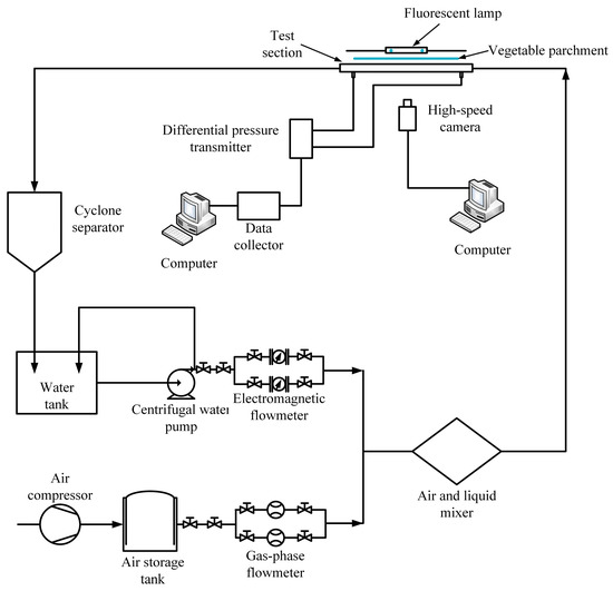
Figure 1.
Experimental system.
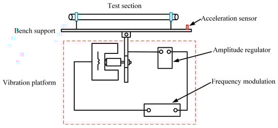
Figure 2.
Vibration device.
We extracted the water from the water tank using the water pump and passed it via a stop valve, electromagnetic flowmeter, and needle valve before entering the gas–water mixer. After the centrifugal pump was provided with a bypass to return to water tank, we adjusted the pressure of this water loop by adjusting the degrees of opening of the bypass valve. The pressure of water loop was displayed by a pressure gauge installed on the main channel. An electromagnetic flowmeter measured the flow of water.
The air was compressed by an air compressor and enters the gas loop through the gas storage tank. The pressure of air loop was displayed by a pressure gauge installed on main channel. The pressure valve was installed in front of the pressure gauge. The gas mass flowmeter measured the gas flow.
The air and water fluid fully blended in the liquid mixer, passed through the experimental test channel in a two-phase state, and entered the cyclone separator. The air phase was directly discharged into the atmosphere. The water phase entered the tank for recycling.
The gas phase conversion flow velocity Jg was 0.1–20 m/s, and the liquid phase conversion flow velocity Jw was 0.1–3.0 m/s. The pipe was placed on the vibrating table horizontally. Table 1 shows the selection of vibration frequency H and amplitude A considers the practical significance of the project and analyses in the previous literature.

Table 1.
Vibration frequency and amplitude selection under transverse vibration.
2.2. Measurements
The measured parameters in our experiment were the fluid velocity and air–water pressure drop. Differential pressure transducers measured the total pressure drop, ΔPtotal. Flow meters measured flow velocity of air and water. A data acquisition system simultaneously recorded the data obtained by the pressure difference transducer and flow meters.
3. Data Reduction
This section provides concise and precise descriptions of the data processing method.
The mass flux G equals the value of mass flow rate divided by the channel cross section area.
The ΔPtotal includes the acceleration pressure drop ΔPa, the frictional pressure drop ΔPf, and the gravity pressure drop ΔPg:
where the ΔPa is [40]
where the void fraction α is obtained by Equation (4) [26].
where the vapor quality x can be expressed as
For air–water flow, the ΔPtotal equals the total of the ΔPa, the ΔPf, and the ΔPg. For the flow in horizontal channel, the ΔPg equals 0.
Thus, we subtracted the ΔPa from the ΔPtotal. We calculated the ΔPf using the following formula:
4. Uncertainty Analysis
According to the literature [41], the experiment’s uncertainty includes Class A and Class B uncertainty. Class A uncertainty is evaluated based on statistical methods and expressed by standard deviation, representing the probability density of the frequency distribution of experimental data. Class B uncertainty is evaluated based on the distribution hypothesis, which represents the half-width of a certain confidence level interval and generally reflects the measurement accuracy of the measuring instrument. Class A uncertainty is calculated as follows:
The calculation method of Class B uncertainty evaluation is based on the distribution hypothesis. This paper’s measurement results adopt the uniform distribution hypothesis; that is, the measured values have equal opportunities in all places within the confidence interval [a−, a+]. The half width of the calculated interval is
where a is also the instrument precision, so the calculation method of Class B evaluation of uncertainty is
where k is the confidence factor.
The calculation for the total measurement uncertainty Uc is as follows:
The range and uncertainties of the measuring instruments and parameters in the two-phase experiment are shown in Table 2. The uncertainties of the pipe diameter and length were measuring errors from the instruments.
Table 2.
The range and uncertainties of the measuring instruments and parameters.
5. Results and Discussion
By observing pictures obtained by the highspeed camera and analyzing them, we obtained five air–water flow patterns. Figure 3 shows the air–water flow patterns under transverse vibration situations differ from those under steady-state conditions in horizontal channel. Air–water flow patterns mainly include the bubble flow, slug flow, stratified flow, wave flow, and annular flow. Figure 3 was developed based on the condition of frequency at 0.8 Hz and the amplitude at 80 mm.
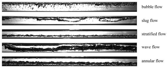
Figure 3.
High-speed photos obtained by the highspeed camera.
5.1. Analysis of the Frictional Pressure Drop
We subtracted the ΔPa and ΔPf and from the ΔPtotal. We also studied the parameters of flow velocity, amplitude, and frequency on the air–water ΔPf.
5.1.1. Flow Fluctuation of the Pressure Drop
Figure 4 and Figure 5 display the fluctuation of the ΔPf of air–water at various frequencies and amplitude, respectively. We analyzed the effects of the frequency and amplitude. Figure 4 shows the vibrational characteristics of ΔPf become more intense with the increase in frequency; this occurs because the increasing frequency increases the instantaneous average speed of air and water. With the increase in the average velocity of air and water, the applied force between the two-phase fluid and the inner wall becomes larger. Then, the vibrational characteristics of ΔPf become intense. As seen in Figure 5, the vibrational characteristics of ΔPf also become more intense with the increase in amplitude because gas–liquid interface collision intensifies with the increasing amplitude. The average speed of air and water becomes larger. Thus, the increasing frequency and amplitude leads to a more intense vibrational characteristic of ΔPf.
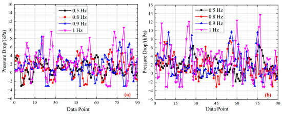
Figure 4.
Different stages of flow instability at various frequency (Jw = 1.1 m/s): (a) Jg = 1.0 m/s, A = 62 mm, (b) Jg = 1.0 m/s, A = 106 mm.
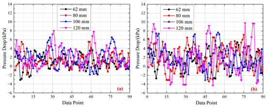
Figure 5.
Different stages of flow instability at various amplitude (Jw = 1.1 m/s): (a) Jg = 1.0 m/s, H = 0.5 Hz, (b) Jg = 1.0 m/s, H = 0.8 Hz.
5.1.2. Comparison of the Characteristics under Vibrational State and Non-Vibrational State
Figure 6 shows the ΔPf of air–water versus the liquid phase conversion flow velocity under vibrational and non-vibrational states. We analyzed the effect of vibration. As seen in Figure 6, ΔPf under the vibrational state is bigger than the value under the non-vibrational state.
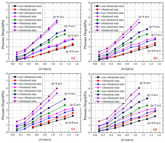
Figure 6.
The pressure drop under vibrational state and non-vibrational state (A = 62 mm): (a) H = 0.5 Hz, (b) H = 0.8 Hz, (c) H = 0.9 Hz, (d) H = 1.0 Hz.
Also, there are some causes for the increased ΔPf caused by vibration. Firstly, the additional vibration force increases the interaction effect between fluid micro-clusters and the wall surface, increasing the friction between the micro-clusters and channel wall. Secondly, the additional vibration force enhances the acting force between air and water, resulting in a more apparent slipping effect between air and water, and even the phenomenon of air shuttling in the water. Thus, the ΔPf under the vibrational state is bigger than the value under the non-vibrational state.
5.1.3. Effect of Flow Velocity
Figure 7 shows the ΔPf of air–water versus the liquid phase conversion flow velocity under various frequencies. We studied the impact of flow velocity on the ΔPf. As shown in Figure 7, ΔPf increases with the increased fluid velocity; this can be interpreted as the air–water average velocity increasing with the increase in fluid velocity. The acting force of the two-phase fluid and the inner wall increases with the air–water average velocity. Thus, the ΔPf increases.
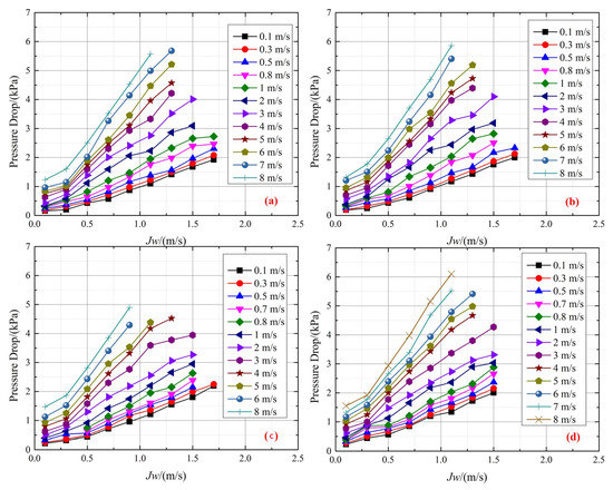
Figure 7.
Effect of flow velocity on the ΔPf (A = 62 mm): (a) H = 0.5 Hz, (b) H = 0.8 Hz, (c) H = 0.9 Hz, (d) H = 1.0 Hz.
Figure 8 shows the ΔPf of air–water versus the liquid phase conversion flow velocity under various amplitudes. As shown in Figure 8, a higher flow velocity results in a bigger ΔPf; thus, a larger flow velocity induces a bigger frictional force between the fluid and the pipe, resulting in a bigger ΔPf. This finding is consistent with most studies [6,14]. As seen in Figure 7 and Figure 8, the ΔPf decreases with the decreasing gas phase conversion flow velocity. The void fraction becomes larger with the increasing gas phase conversion flow velocity, leading to a thinner water film near the pipe wall. The vapor flow velocity is higher at larger void fraction, resulting in a bigger ΔPf.
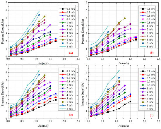
Figure 8.
The effect of flow velocity on the ΔPf (H = 0.8 Hz): (a) A = 62 mm, (b) A = 80 mm, (c) A = 106 mm, (d) A = 120 mm.
Also, when the conversion velocity of air is small, the flow is basically in bubble flow, and the ΔPf is small. The additional force generated by vibration shows little impact on the air–water fluid, so the ΔPf changes slightly.
When the conversion velocity of gas phase conversion is at a high value, the flow is basically in slug and wave flow. Under the impact of the additional force obtained by vibration, the air shuttles in the water, increasing the air and water phase interforce and energy dissipation. As a result, the ΔPf increases significantly.
5.1.4. Effect of the Amplitude
Figure 9 displays the ΔPf versus the liquid phase conversion flow velocity at various amplitudes. We analyzed the effect of amplitude. As seen in Figure 9, the ΔPf increases with the increasing amplitude. The increase in amplitude increases the additional vibration force. Thus, the interaction effect between fluid micro-clusters and the wall surface increases, leading to friction between fluid micro-clusters and the channel wall. Moreover, the additional vibration force enhanced the interaction between the air and water phases, resulting in a more apparent slipping effect between air and water and even the phenomenon of air shuttling in water. Thus, the ΔPf increases with the increasing amplitude.
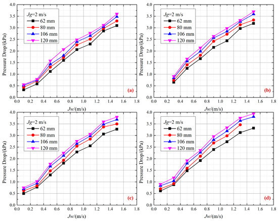
Figure 9.
Effect of amplitude on ΔPf: (a) H = 0.5 Hz, (b) H = 0.8 Hz, (c) H = 0.9 Hz, (d) H = 1.0 Hz.
5.1.5. Effect of the Frequency
Figure 10 shows ΔPf versus the liquid phase conversion flow velocity at various frequencies. We analyzed the effect of frequency. As seen in Figure 10, the ΔPf increases with the increasing frequency. The increase in frequency increases the additional vibration force. Thus, the interaction effect between fluid micro-clusters and the wall surface increases, leading to friction between fluid micro-clusters and the channel wall. Furthermore, the additional vibration force enhances the interaction between air and water, resulting in a more apparent slipping effect between air and water and even the phenomenon of the air shuttling in water phase. Thus, the ΔPf increases with the increasing frequency.
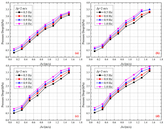
Figure 10.
The effect of frequency on ΔPf: (a) A = 62 mm, (b) A = 80 mm, (c) A = 106 mm, (d) A = 120 mm.
5.2. Analysis on Correlations
5.2.1. Evaluation of Existing Correlations
Lockhart and Martinelli proposed liquid multiplier ϕL2 to characterize the characteristics of two-phase fluid flow. As shown in Equation (11), the liquid multiplier is equal to the ΔPf divided by the liquid-phase pressure drop ΔPL. The liquid multiplier is related to steam mass, fluid density, and viscosity:
where ΔPL is the pressure drop when only liquid flows in the channel, calculated by Blasius correlation. C coefficient is a value that relates to the flow characteristics of the two phases.
Table 2 shows the previous frictional pressure drop correlations. These models can calculate their own experimental results independently; however, the results of air–water experiments under lateral vibration conditions are uncertain and must be studied.
We used the homogeneous mixture and separated model to evaluate the experimental results of ΔPf. The ΔPf calculation formula under the homogeneous mixture model is
A separate flow model was used to predict ΔPf, as well as the Lockhart and Martinelli methods, which can be represented as
The comparison results between the predictive models and experimental data are shown in Figure 11. The ΔPf were calculated with the Lockhart–Martinelli, Dukler [42], Chisholm, Friedel, homogeneous, and Muller and Heck [43] models.
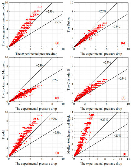
Figure 11.
Comparison between the experimental values and the calculated values based on different correlations: (a) Homogenous; (b) Dukler; (c) Lockhart–Martinelli; (d) Chisholm B coefficient; (e) Friedel; (f) Muller and Heck.
The comparison between the calculated results of these correlations and experimental results with mean absolute deviation (MAD) and mean relative deviation (MRD) is presented. The deviations between the experimental results and the results calculated by these models are listed in Table 3.
Table 3.
The comparison between experiment results and these correlations.
As listed in Table 1, the data calculated by correlations proposed by Dukler and Chisholm can predict the experimental results well, as reflected by a MAD of ±20%. Among these correlations, the one from Dukler predicts the ΔPf of air–water better than the other correlations. The poor predictions from these correlations for the ΔPf, as shown in Table 2, result from deviations in the reduced pressure, channel diameter, shape of the channel, and flow condition between those studies and this study.
5.2.2. The New Proposed Correlation
From the above analysis, the air–water frictional pressure drop value under the transverse vibration condition in the horizontal channel by the existing correlation coefficient is slightly higher or lower. Therefore, we propose a new correlation considering reasonable parameters to improve the prediction accuracy. As shown in Equation (7), the C coefficient improves the correlation’s prediction of experimental data, and the C value relates to the flow characteristics of the fluid. Therefore, to consider reasonable parameters, we established the C coefficient correlation.
The confinement number Co, which listed in Equation (16), is considered in the newly developed correlation.
As shown in Figure 12, C-coefficient changes with the variation in x. Hence, the newly modified correlation should consider the effect of x on the ΔPf.
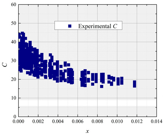
Figure 12.
The comparison of coefficient C of air–water and the vapor quality.
Coefficient C is newly modified as Equation (17). It contains the effect of Co, x, the frequency H, and amplitude A on the frictional pressure drop.
Based on the frictional pressure drop’s experimental values, we calculated those of the liquid-phase multiplier with Equations (11) and (13). The fluid properties at each operating point were obtained by REFPROP 9 software. Therefore, the X, calculated by Equation (11), was obtained. Thus, we obtained the experimental value of C based on Equation (11). We calculated the values of vapor quality x and Co using Equations (5) and (16) at each operating point. Therefore, based on Equation (17), the coefficients of a1, a2, a3, a4 and a5 were obtained; the values are a1 = −0.08135, a2 = 0.96301, a3 = 0.54807, a4 = −79.90416, a5 = 0.83409.
Figure 13 shows the values of the ΔPf calculated by newly developed correlation. Table 4 lists the experimental ΔPf deviation calculated by the developed model. The newly developed model is superior to the Dukler correlation in predicting experimental results under lateral vibration. For the newly developed correlation, the MAD and MRD are 8.2 and 1.4%.
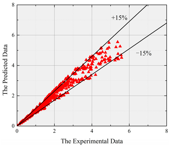
Figure 13.
Comparison of the experimental ΔPf and the calculated results based on modified correlation.
Table 4.
Comparison of the results of the newly modified correlation and Dukler correlation.
The relative deviation (RD) is used to analyze the deviation of each experimental value. It can be expressed as
where p(j)pred is the calculated results, p(j)exp is the experimental results.
Figure 14 displays the variation in RD versus x. The results show that as the newly modified correlation considers the effect of x, the impact of x on the performance of the newly modified correlation is minor.
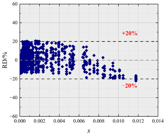
Figure 14.
The relative deviation versus the vapor quality by using the newly developed correlation.
5.2.3. Comparison with Other Literature Data
We amassed published pressure drop databases from two sources in the present study. Details on these studies are shown in Table 5, with 255 pressure drop data points.
Table 5.
Pressure drop data included in the database.
Figure 15 compares the calculated data of newly developed correlation and experimental data from the other literature. The newly modified correlation predicts the other three studies accurately. The MRD and MAD for these studies are −3.6% and 25.8%, respectively.
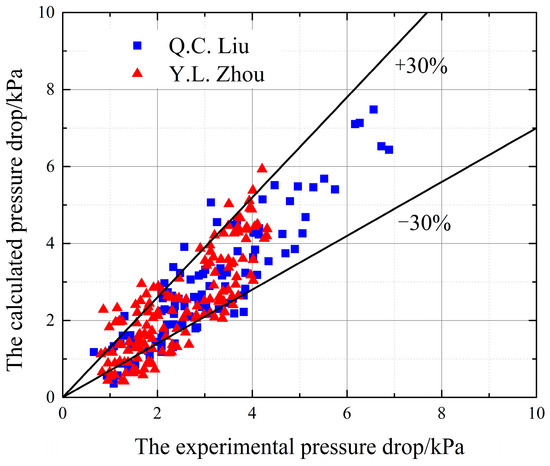
Figure 15.
The comparison between the calculated values of developed correlation and the experimental values.
The content of this research can be summarized as follows: The newly modified correlation can predict the experimental results of the other literatures; however, its error is a little bigger and it lacks a comprehensive study of different pipe diameters, flow directions, and vibration directions. In future studies, we plan to combine the fitting correlation formula in this paper with other vibration conditions to obtain a unified correlation under different vibration conditions. Moreover, we intend to deeply study the variation flow characteristics under different flow patterns and establish a flow pattern recognition theory based on the pressure signal.
6. Conclusions
We experimentally analyzed the air–water flow characteristics under stable and transverse vibration conditions in the horizontal pipes with inner diameters of 20 mm.
- (1)
- With increases in frequency and amplitude, the vibrational characteristics of frictional pressure drops become more intense. The pressure drop under vibrational state is bigger than that under the non-vibrational state. Moreover, the pressure drop values relate to the fluid velocity, transverse vibration frequency, and transverse vibration amplitude. The variation characteristic of the air–water pressure drop is strongly affected by flow velocity. The pressure drop enlarges as the flow velocity become larger;
- (2)
- The previous correlations were divided into homogenous correlation and the separated flow correlation. We evaluated the accuracy of these correlations by comparing these correlations with the present experimental results. Among all these correlations, the Dukler correlation showed the best forecast results with the MAD of 20%;
- (3)
- We proposed a modified Chisholm relation predicting the air–water two-phase pressure drop under transverse vibration conditions. We considered the influence of confinement number, vapor quality, amplitude, and frequency on coefficient C in this modified correlation. The newly modified correlation showed better performance for predicting the experimental results. The MAD and MRD were 8.2 and 1.4%. Moreover, the newly modified correlation predicts the other three studies accurately.
Author Contributions
Methodology, B.S.; Validation, Y.Z.; Formal analysis, B.S. and Y.Z.; Data curation, B.S.; Writing—original draft, B.S.; Writing—review & editing, Y.Z. All authors have read and agreed to the published version of the manuscript.
Funding
This research was funded by Natural Science Foundation of China, grant number 51776033 and 51541608.
Data Availability Statement
Readers can contact the author through the email address for the experimental data.
Conflicts of Interest
The authors declare no conflict of interest.
References
- Gong, H.; Xiao, Y.; Yang, Y.H.; Xiao, Z.J. Experimental research of bubble characteristics in narrow rectangular channel under heaving motion. Int. J. Therm. Sci. 2012, 51, 42–50. [Google Scholar]
- Alonso, B.A.; Meneley, D.A.; Misak, J.; Bleed, T.; van Erp, J.B. Why nuclear energy is sustainable and has to be part of the energy mix. Sustain. Mater. Technol. 2014, 1, 8–16. [Google Scholar]
- Zhou, Y.L.; Chang, H. Gas-liquid two-phase flow in a horizontal channel under nonlinear oscillation: Flow regime, frictional pressure drop and void fraction. Exp. Therm. Fluid Sci. 2019, 109, 109852. [Google Scholar] [CrossRef]
- Kharti, K.M.; Alishahi, M.; Emdad, H. Analysis of pressure field in time domain using nonlinear reduced frequency approach in unsteady transonic flows. Int. J. Num. Methods Heat Fluid Flow 2010, 20, 655–669. [Google Scholar] [CrossRef]
- Yu, J.C.; Li, Z.X.; Zhao, T.S. An analytical study of laminar heat convection in a circular pipe with constant heat flux. Int. J. Heat Mass Transf. 2004, 47, 5297–5301. [Google Scholar] [CrossRef]
- Wu, J.; Koettig, T.; Franke, C.; Helmer, D.; Eisel, T.; Haug, F.; Bremer, J. Investigation of heat transfer and pressure drop of CO2 two-phase flow in a horizontal minichannel. Int. J. Heat Mass Transf. 2011, 54, 2154–2162. [Google Scholar] [CrossRef]
- Pamitran, A.S.; Choi, K.-I.; Oh, J.-T.; Oh, H.-K. Two-phase pressure drop during CO2 vaporization in horizontal smooth minichannels. Int. J. Refrig. 2008, 31, 1375–1383. [Google Scholar] [CrossRef]
- Choi, K.-I.; Pamitran, A.S.; Oh, C.-Y.; Oh, J.-T. Two-phase pressure drop of R-410A in horizontal smooth minichannels. Int. J. Refrig. 2008, 31, 119–129. [Google Scholar] [CrossRef]
- Yang, C.Y.; Webb, R.L. Friction pressure drop of R-12 in small hydraulic diameter extruded aluminum tubes with and without micro-fins. Int. J. Heat Mass Transf. 1996, 39, 801–809. [Google Scholar] [CrossRef]
- Hwang, Y.W.; Kim, M.S. The pressure drop in microtubes and the correlation development. Int. J. Heat Mass Transf. 2006, 49, 1804–1812. [Google Scholar] [CrossRef]
- Steiner, D.; Schlünder, E.U. Heat transfer and pressure drop for boiling nitrogen flowing in a horizontal tube:1. Saturated flow boiling. Cryogenics 1976, 16, 387–398. [Google Scholar] [CrossRef]
- Steiner, D. Heat transfer and pressure drop for boiling nitrogen flowing in a horizontal tube: 2. Pressure drop. Cryogenics 1976, 16, 457–464. [Google Scholar] [CrossRef]
- Filippov, Y.P. Characteristics of horizontal two-phase helium flows: Part II: Pressure drop and transient heat transfer. Cryogenics 1999, 39, 69–75. [Google Scholar] [CrossRef]
- Chen, D.; Shi, Y. Two-phase heat transfer and pressure drop of LNG during saturated flow boiling in a horizontal tube. Cryogenics 2013, 58, 45–54. [Google Scholar] [CrossRef]
- Chen, D.; Shi, Y. Study on two-phase pressure drop of LNG during flow boiling in a 8 mm horizontal smooth tube. Exp. Therm. Fluid Sci. 2014, 57, 235–241. [Google Scholar] [CrossRef]
- Buscher, S. Two-phase pressure drop and void fraction in a cross-corrugated plate heat exchanger channel: Impact of flow direction and gas-liquid distribution. Exp. Therm. Fluid Sci. 2021, 126, 110380. [Google Scholar] [CrossRef]
- Cai, B.; Xia, G.; Cheng, L.; Wang, Z. Experimental investigation on spatial phase distributions for various flow patterns and frictional pressure drop characteristics of gas liquid two-phase flow in a horizontal helically coiled rectangular tube. Exp. Therm. Fluid Sci. 2023, 142, 110806. [Google Scholar] [CrossRef]
- Doyle, B.; Riviere, B.; Sekachev, M. A multinumerics scheme for incompressible two-phase flow. Comput. Methods Appl. Mech. Eng. 2020, 370, 113213. [Google Scholar] [CrossRef]
- Ferraris, D.L.; Marcel, C.P. Two-phase flow frictional pressure drop prediction in helical coiled tubes. Int. J. Heat Mass Transf. 2020, 162, 120372. [Google Scholar] [CrossRef]
- Xing, D.C.; Yan, C.Q.; Sun, L.C.; Wang, C. Effect of rolling motion on single-phase laminar flow resistance of forced circulation with different pump head. Ann. Nucl. Energy 2013, 54, 141–148. [Google Scholar] [CrossRef]
- Yu, Z.T.; Tan, S.C.; Yuan, H.S.; Chen, C.; Chen, X.B. Experimental investigation on flow instability of forced circulation in a mini-rectangular channel under rolling motion. Int. J. Heat Mass Transf. 2016, 92, 732–742. [Google Scholar] [CrossRef]
- Jin, G.; Yan, C.; Sun, L.; Xing, D. Effect of rolling motion on transient flow resistance of two-phase flow in a narrow rectangular duct. Ann. Nucl. Energy 2014, 64, 135–143. [Google Scholar] [CrossRef]
- Li, S.; Cai, W.; Jiang, Y.; Zhang, H.; Li, F. The pressure drop and heat transfer characteristics of condensation flow with hydrocarbon mixtures in a spiral pipe under static and heaving conditions. Int. J. Refrig. 2019, 103, 16–31. [Google Scholar] [CrossRef]
- Iliuta, I.; Larachi, F. CO2 and H2S absorption by MEA solution in packed-bed columns under inclined and heaving motion conditions—Hydrodynamics and reactions performance for marine applications. Int. J. Greenh. Gas Control 2018, 79, 1–13. [Google Scholar] [CrossRef]
- Pendyala, R.; Jayanti, S.; Balakrishnan, A.R. Flow and pressure drop fluctuations in a vertical tube subject to low frequency oscillations. Nucl. Eng. Des. 2008, 238, 178–187. [Google Scholar] [CrossRef]
- Cicchitti, A.; Lombardi, C.; Silvestri, M.; Soldaini, G.; Zavattarelli, R. Two-phase cooling experiments-pressure drop, heat transfer, and burnout measurements. Energia Nucl. 1960, 7, 407–425. [Google Scholar]
- Lockhart, R.W.; Martinelli, R.C. Proposed correlation of data for isothermal two-phase, two-component flow in pipes. Chem. Eng. Prog. 1949, 45, 39–48. [Google Scholar]
- Chisholm, D. A theoretical basis for the Lockhart-Martinelli correlation for two-phase flow. Int. J. Heat Mass Transf. 1967, 10, 1767–1778. [Google Scholar] [CrossRef]
- Friedel, L. Improved friction drop correlations for horizontal and vertical two phase pipe flow. Proc. Eur. Two-Phase Flow Group Meet. 1979, 8, 2. [Google Scholar]
- Yan, Y.Y.; Lin, T.F. Evaporation heat transfer and pressure drop of refrigerant R-134a in a small pipe. Int. J. Heat Mass Transf. 1998, 41, 4183–4194. [Google Scholar] [CrossRef]
- Sun, L.; Mishima, K. Evaluation analysis of prediction methods for two-phase flow pressure drop in mini-channels. Int. J. Multiph. Flow 2009, 35, 47–54. [Google Scholar] [CrossRef]
- Li, W.; Wu, Z. A general correlation for adiabatic two-phase pressure drop in micro/mini-channels. Int. J. Heat Mass Transf. 2010, 53, 2732–2739. [Google Scholar] [CrossRef]
- Zhang, W.; Hibiki, T.; Mishima, K. Correlations of two-phase frictional pressure drop and void fraction in mini-channel. Int. J. Heat Mass Transf. 2010, 53, 453–465. [Google Scholar] [CrossRef]
- Ungar, E.; Cornwell, J. Two-phase pressure drop of ammonia in small diameter horizontal tubes. In Proceedings of the 28th Joint Propulsion Conference and Exhibit, Nashville, TN, USA, 6–8 July 1992. [Google Scholar]
- Aakenes, F.; Munkejord, S.T.; Drescher, M. Frictional Pressure Drop for Two-phase Flow of Carbon Dioxide in a Tube: Comparison between Models and Experimental Data. Energy Procedia 2014, 51, 373–381. [Google Scholar] [CrossRef]
- Mishima, K.; Hibiki, T. Some characteristics of air–water two-phase flow in small diameter vertical tubes. Int. J. Multiph. Flow 1996, 22, 703–712. [Google Scholar] [CrossRef]
- Kim, S.-M.; Mudawar, I.S. Universal approach to predicting two-phase frictional pressure drop for mini/micro-channel saturated flow boiling. Int. J. Heat Mass Transf. 2013, 58, 718–734. [Google Scholar] [CrossRef]
- Liu, Q.; Zhou, Q.; Chen, C. Frictional pressure drop of gas-liquid two-phase flow in vertical and inclined upward tubes under heaving oscillation. Int. Commun. Heat Mass Transf. 2022, 135, 106108. [Google Scholar] [CrossRef]
- Milićević, A.R.; Belošević, S.V.; Tomanović, I.D. Development of mathematical model for co-firing pulverized coal and biomass in experimental furnace. Therm. Sci. 2018, 22, 709–719. [Google Scholar] [CrossRef]
- Thome, J.R. Engineer Data Book III; Wolverine Tube Inc.: Decatur, AL, USA, 2006. [Google Scholar]
- Moffat, R.J. Describing the uncertainties in experimental results. Exp. Therm. Fluid Sci. 1988, 1, 3–17. [Google Scholar] [CrossRef]
- Dukler, A.E.; Wicks, M.; Cleveland, R.G. Pressure drop and hold-up in two-phase flow—Part A: A comparison of existing correlations. AIChE J. 1964, 10, 38–43. [Google Scholar] [CrossRef]
- Müller-Steinhagen, H.; Heck, K. A simple friction pressure drop correlation for two-phase flow in pipes. Chem. Eng. Process. Process Intensif. 1986, 20, 297–308. [Google Scholar] [CrossRef]
Disclaimer/Publisher’s Note: The statements, opinions and data contained in all publications are solely those of the individual author(s) and contributor(s) and not of MDPI and/or the editor(s). MDPI and/or the editor(s) disclaim responsibility for any injury to people or property resulting from any ideas, methods, instructions or products referred to in the content. |
© 2022 by the authors. Licensee MDPI, Basel, Switzerland. This article is an open access article distributed under the terms and conditions of the Creative Commons Attribution (CC BY) license (https://creativecommons.org/licenses/by/4.0/).