
Applications and Modeling Techniques of Wind Turbine Power Curve for Wind Farms—A Review

 , ,
, ,  ,
, 

Abstract
:1. Introduction
- A large portion of the modeling techniques requires optimal (normal) historical data to be available in advance for model learning purposes. Yet, how to attain an optimal (normal) historical data to train and validate the models is completely ignored in the currently available review papers.
- Recent findings have reported a wide range of power curve based anomalies and fault signatures, which is very effective for root cause analysis, diagnosis and prognosis. However, none of the currently available review papers have addressed those recent findings.
- The applications of the wind turbine power curve are explored, including their involvement in the process of wind turbine selection, capacity factor estimation, wind energy assessment and forecasting, and condition monitoring.
- The most common types of power curve based anomaly and fault signatures are investigated and analyzed from a diagnostic standpoint. That includes a wide range of issues, such as those caused by “damaged power measuring instrument”, “communication equipment fault”, “imposed control action”, “load sensor failure”, and “harsh environmental conditions”, among others.
- Data preprocessing and correction schemes, which are usually performed prior to modelling the power curve of wind turbine in order to attain the optimal (normal) historical data, are explored. That includes methods in the framework of filtering, clustering, isolation, and other approaches.
- An updated review of the modeling techniques including parametric and non-parametric algorithms is presented along with the most common performance metrics.
2. Wind Turbine Power Curve
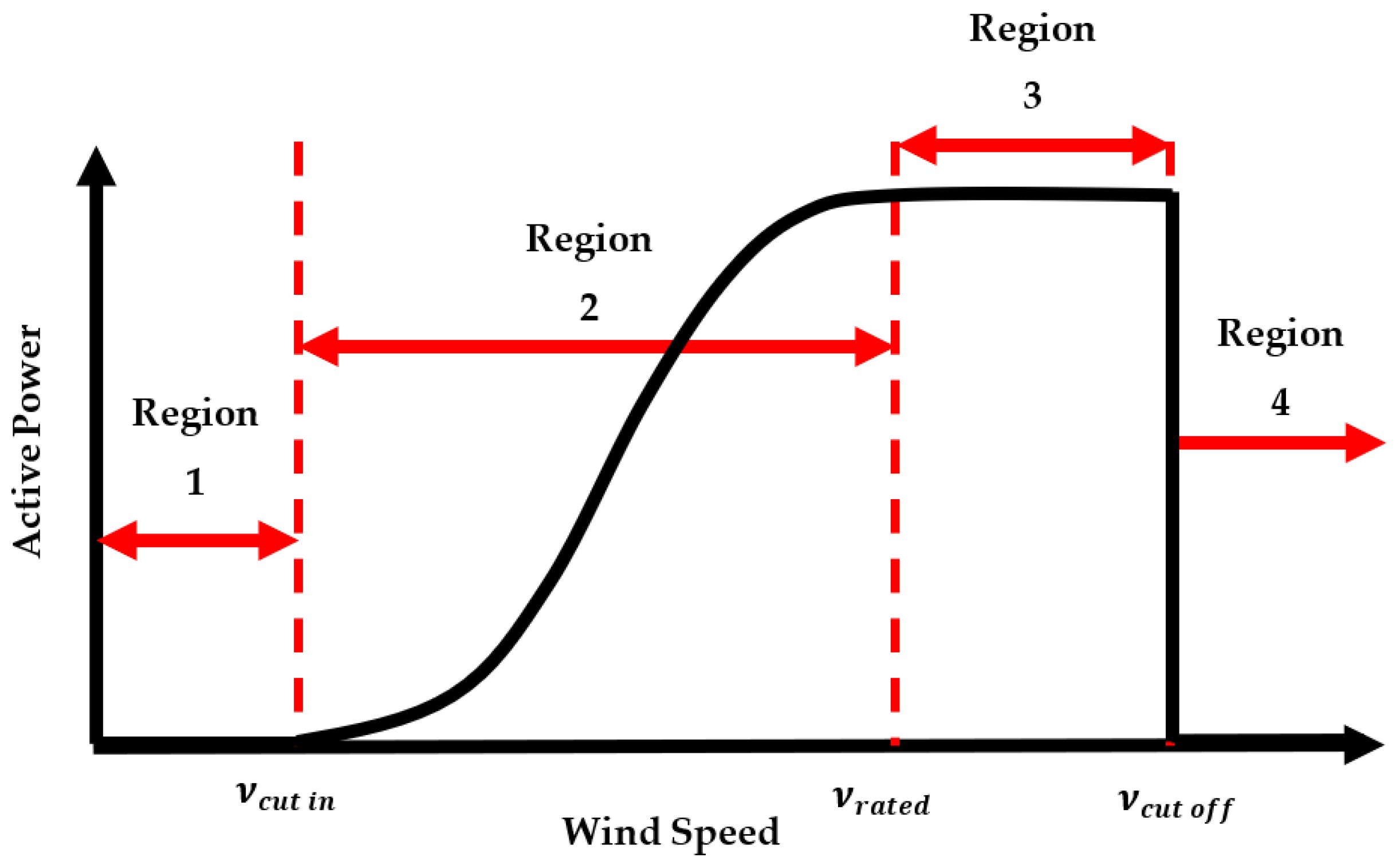
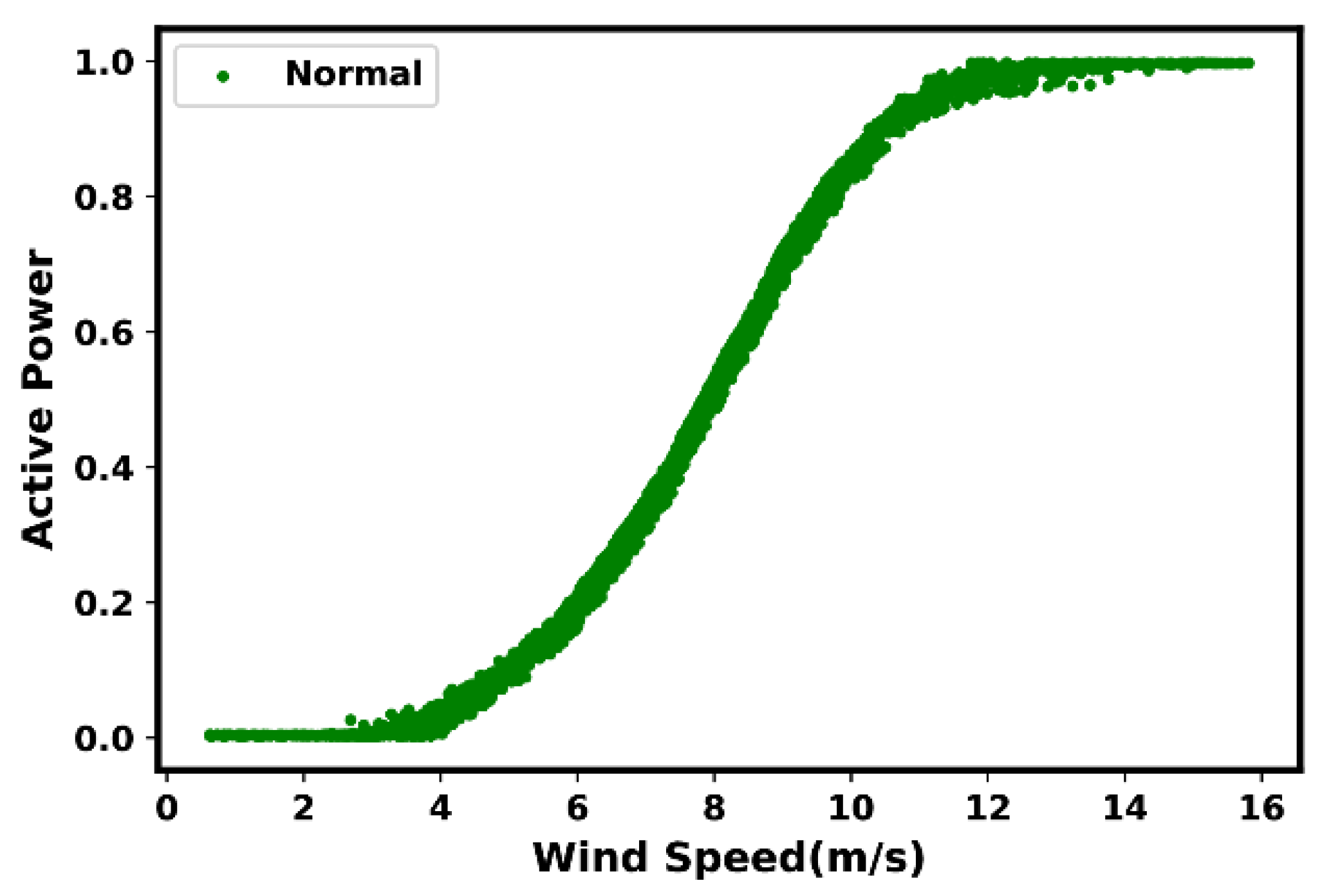
- From a low-level wind speed, the wind turbine doesn’t generate power; power generation commence at the “cut-in speed” ;
- When the wind speed level rises from the “cut-in speed”, the wind turbine generates power at an increasing rate, up to the “rated speed” ;
- Having reached the “rated speed”, the wind turbine generates power at a constant rate, which is the maximum rated power up to the “cut-off speed” ;
- From the “cut-off” speed limit, it is generally turned off as a preventive measure, in order to safeguard the wind turbine from higher speeds which may expose danger and damage the wind turbine seriously.
2.1. Ideal Power Curve
2.2. Actual Power Curve
3. Applications of Power Curve
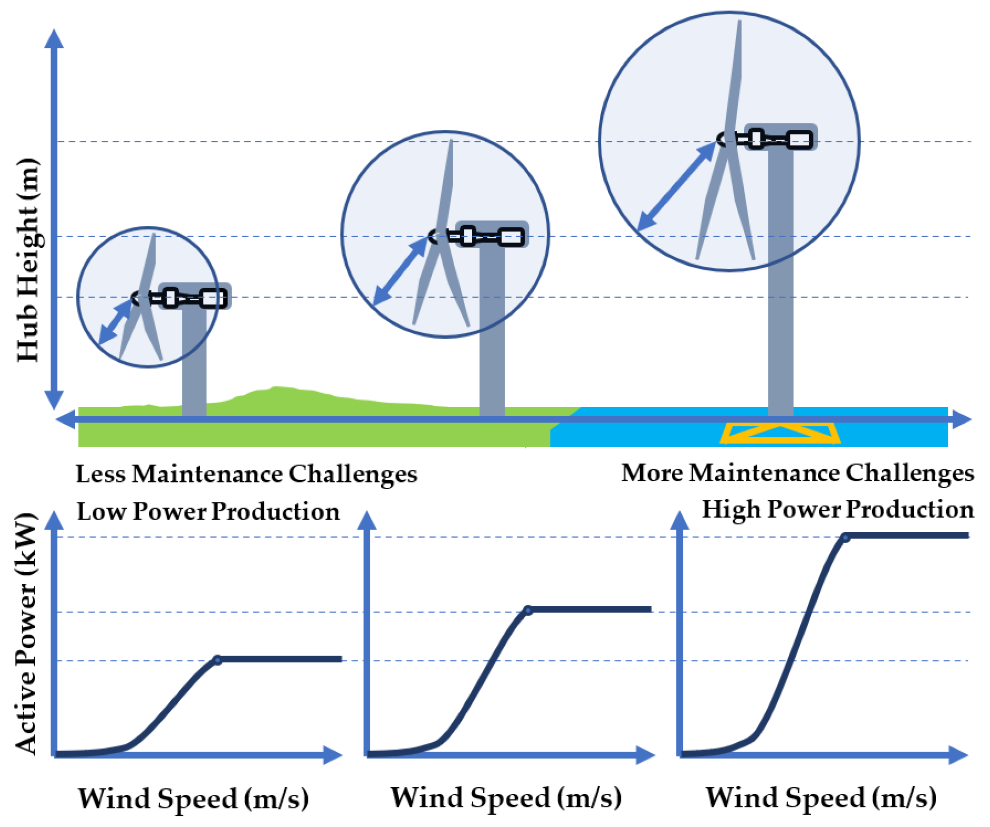
3.1. Wind Turbine Selection
- On one hand, one may notice that, although larger and taller wind turbines are able to produce more power compared with the smaller and shorter ones, larger wind turbines can cause added expenses and delays in maintenance when replacing major components. One of the major challenges is the lack of facilities to lift heavy loads to the top of tall towers.
- On the other hand, smaller wind turbines are apparently easier with regards to maintenance; however, they could provide lower production revenue due to shorter towers or less efficiency in general.
3.2. Capacity Factor Estimation
3.3. Wind Energy Assessment and Forecasting
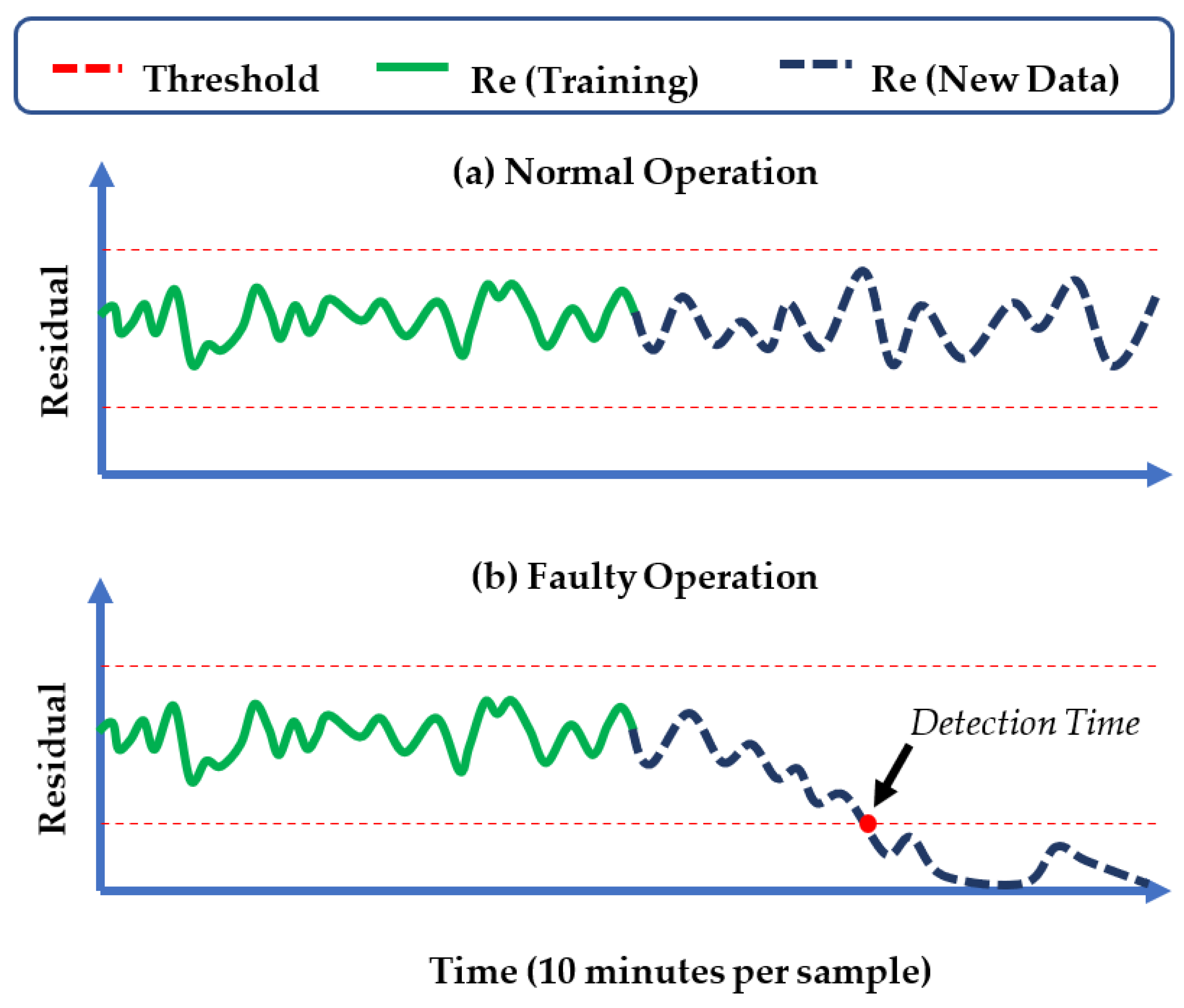
3.4. Condition Monitoring
- If the attained residuals are continuously fluctuating between the established threshold limits, then the wind turbine is considered to be functioning according to the norm;
- Else if the attained residuals rise or descend beyond the established threshold limits, the wind turbine is considered to be experiencing an unusual event. In such cases, the moment when the residual crosses the threshold limit, may be considered as the first detection time.
- Online Condition Monitoring: Online condition monitoring refers to real-time inspections. In this approach, the wind turbine is continuously under observation and often involves automatic systems.
- Offline Condition Monitoring: Offline condition monitoring refers to periodic inspections. In this approach, the wind turbine is required to be “shut down”, and often requires operator’s intervention.
4. Anomaly and Fault Signatures
4.1. Indications of Suboptimal Performance
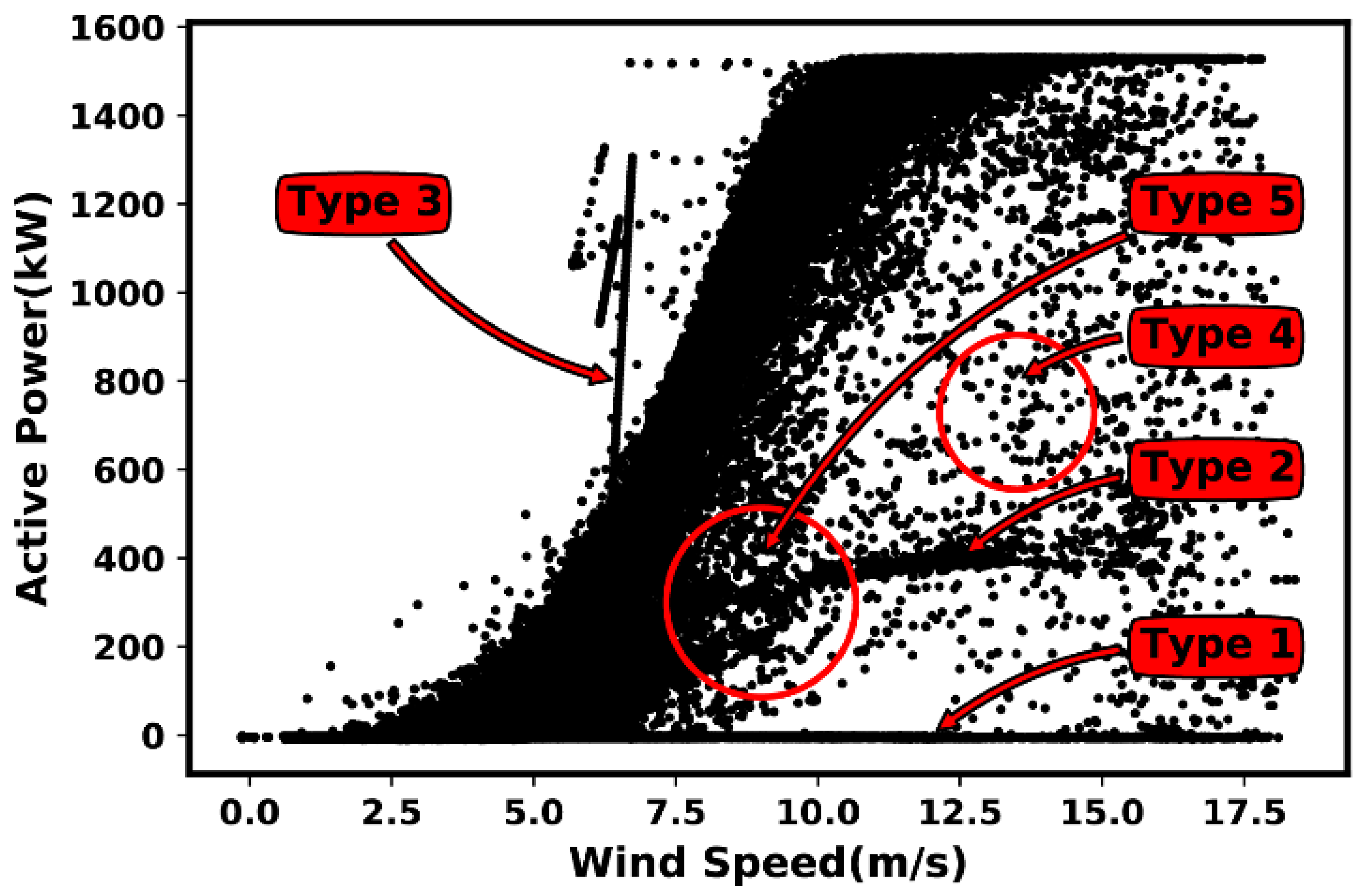
4.2. Most Common Anomaly and Fault Types
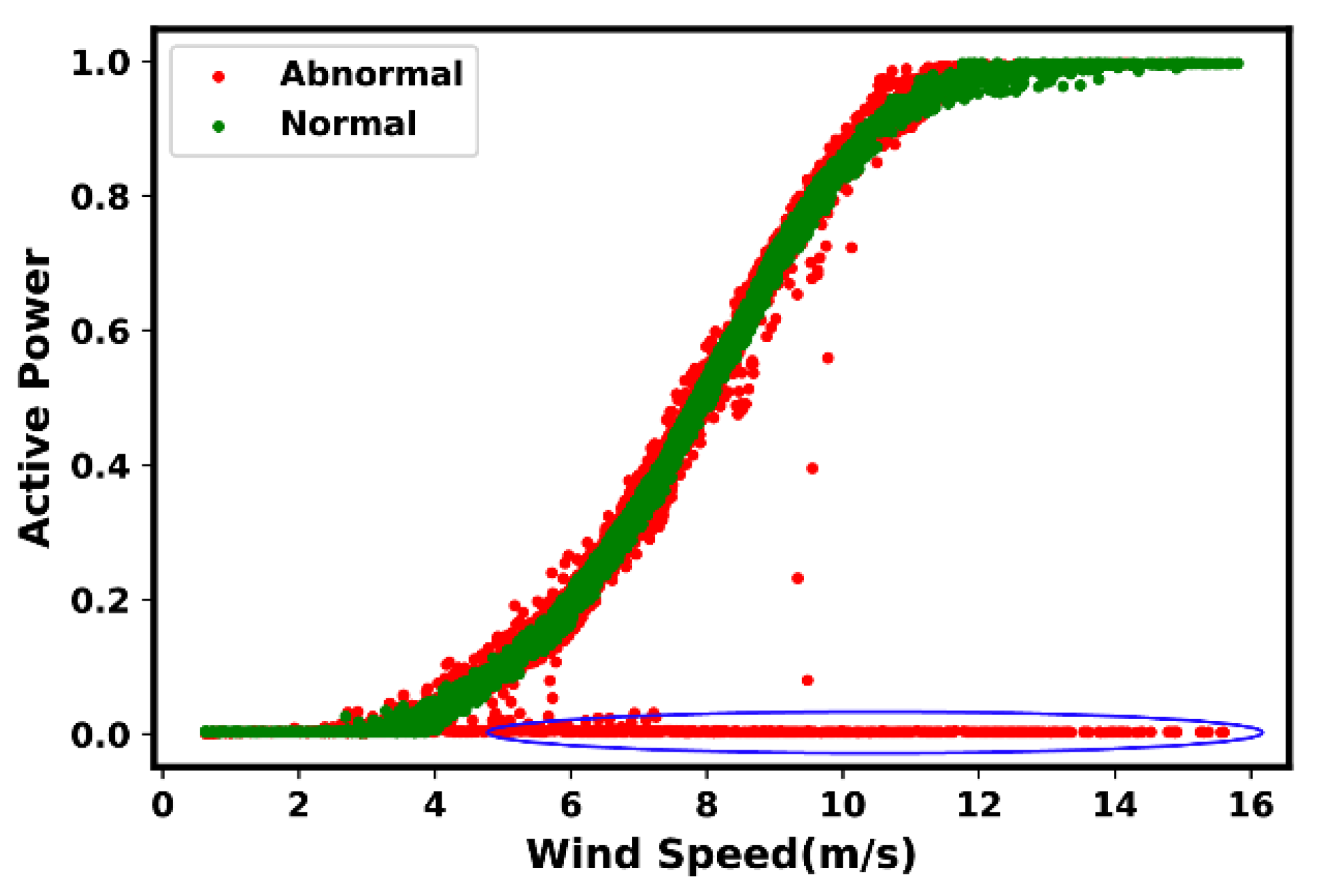
- Type 6: Negative power curve values. Such events are often identifiable through the observed data points below zero.
- Type 7: Overrating. Such situations are true in the presence of data points found above the rated power.
- Blade Fault: Rotor blade surface degradation results in a reduced aerodynamic efficiency, which will cause reduction in power generation of the wind turbine.
- Yaw System Fault: In general, the “yaw system” aims to maintain the wind turbine pointing towards the wind direction properly. Misalignments may result in “lowered airflow” through the wind turbine, and hence, lower power generation. This may take place across the “wind speed” range.
- Pitch System Fault: For pitch regulated wind turbines, and below the “rated wind speed”, the blades generally pitch towards the angle that enables a greater aerodynamic efficiency. Considering “wind speed” above the “rated speed”, the blades pitch to mitigate the fraction of power transferred from the wind and to maintain the rated power. Faulty pitch mechanisms are probably to appear in a greater variability at all “wind speeds” or can result to over-production or under-production of power at higher “wind speeds”.
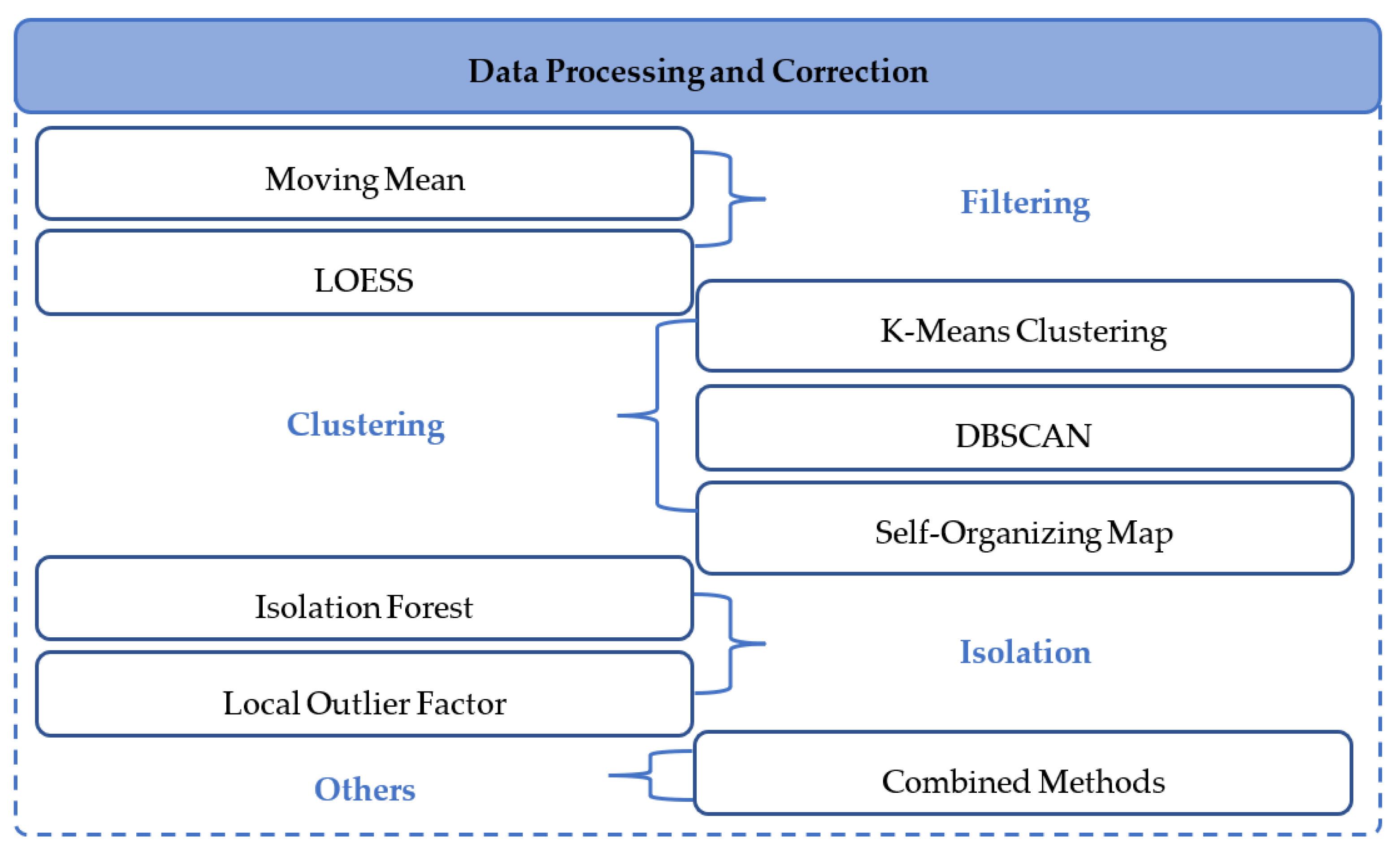
5. Data Preprocessing and Correction
5.1. Filtering Approach
- (a)
- Moving Mean: Extracting a statistical moving mean feature from both signals that essentially constitute the power curve (i.e., “wind speed” and “active power”) can often help to reduced minor stochastic effects found in the dataset. The “moving mean” feature can be obtained by the following mathematical description:
- (b)
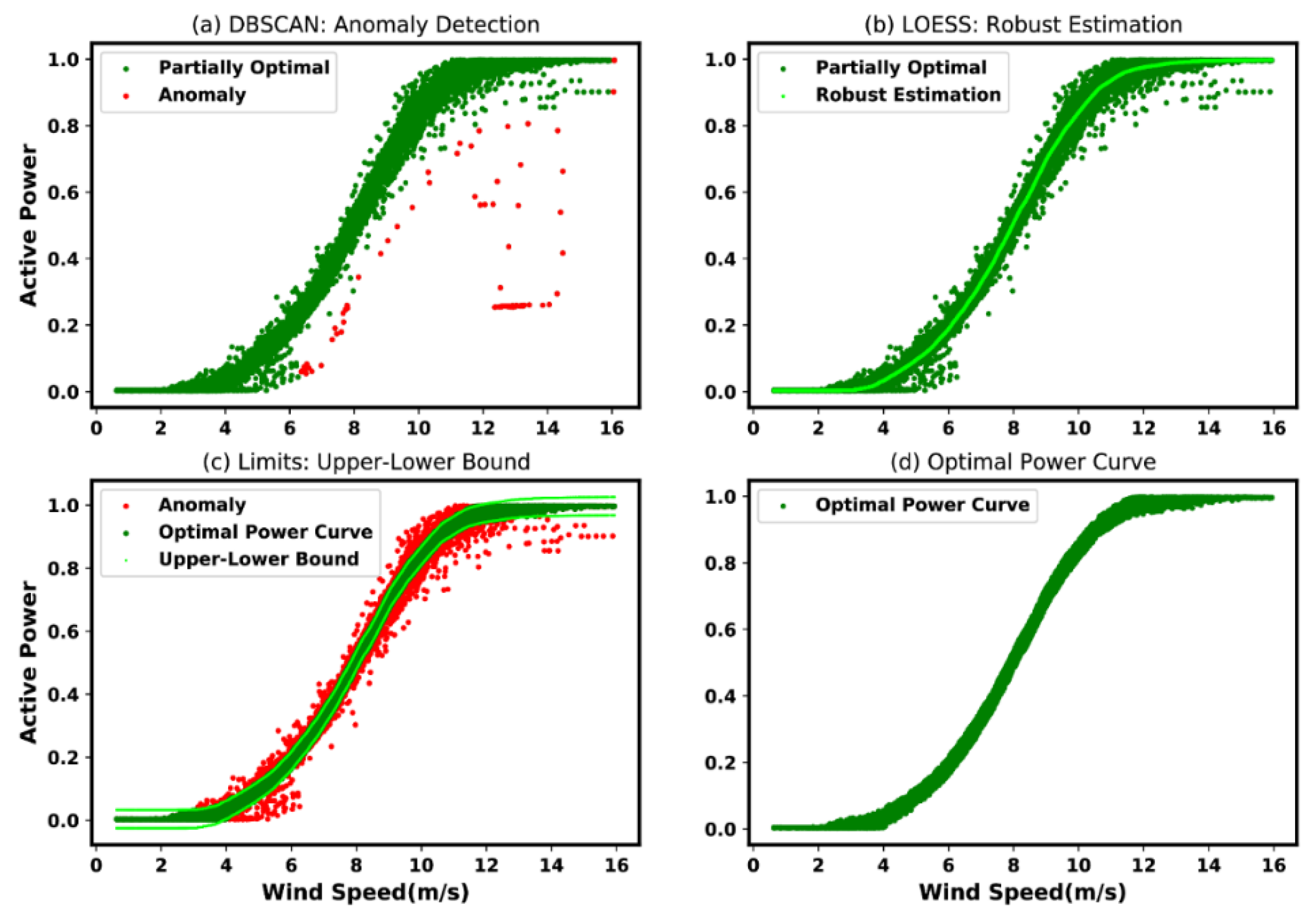
- Locally Weighted Regression (LOESS): Essentially, LOESS is a smoothing algorithm. In LOESS, every smoothened value is determined using the neighboring data points within a given span. The regression weight for each data point in the span is calculated using the following expression:
5.2. Clustering Approach
- (a)
- K-Means Clustering: The “k-means clustering” classifies data by separating samples in clusters of equal variance by applying minimization through a criterion referred to as the “inertia” or “within-cluster sum-of-squares” (WCSS). The number of clusters, however, needs to be specified. In general, it performs well in a large size dataset, and it has been adopted in various application domains. In particular, the “k-means clustering” tends to divide a set of samples into disjoint clusters , each described by the mean of the samples in the cluster. The means of each cluster are generally considered as the centroids of the clusters. The algorithm usually chooses centroids that minimize the WCSS based on the expression:
- (b)
- Density-Based Spatial Clustering of Applications with Noise (DBSCAN): The “DBSCAN” regards clusters as regions of higher density distinct from those with lower density. In this particular approach, which is rather “generic view”, the considered clusters may take on any shapes. In DBSCAN, the “core samples points” are the most essential, which are mainly samples located in the regions of “high density”. Essentially, a considered cluster is, thus, a set of “core samples points” located near each other (calculated based on a “distance metrics”, such as “Eucledian”) and a set of “non-core samples points” that are near to a “core sample point”. The parameters namely, the radius and the minimum sample points, need to be specified in order to define the density. The procedure is shown in Algorithm 1. For instance, this approach (DBSCAN) has been used in [21,74,75] for data correction purpose.
| Algorithm 1: Pseudocode of the original DBSCAN. |
| Input: DB (database), ε (radius), dist(distance function), and minPts(density threshold) |
| Output: labels |
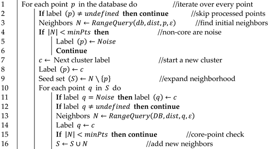 |
- (c)
- Self-Organizing Map (SOM): The so-called SOM is generally an “unsupervised technique” which is usually employed to produce a low-dimensional representation of a higher dimensional dataset while preserving the topological structure of the data. It is widely used for clustering and data dimensionality reduction. The SOM is a typical artificial neural network composed of input layer, output layer, and connection weights. It is trained in an iterative process including competition and convergence. In the th iterative step, the SOM finds the winner in the competition, which is the closest neuron to the input sample . Subsequently, the convergence procedure leads the SOM model adjusting towards the expected order by updating the weight vectors based on the neighborhood relationships with the winner neuron. The neighborhood function that determines the neighbor update scheme for the topology-preserving nature of SOM is usually in the form of Gaussian function:
5.3. Isolation Approach
- (a)
- Isolation Forest (iForest): The iForest is an ensemble of trees; it uses an unsupervised learning approach to detect unusual data points which can subsequently be removed from the training data. Essentially, it performs isolation by a random selection of a feature and subsequently random selection of a split sample between the maximum and minimum samples of the chosen feature. Given the fact that “recursive partitioning” may be depicted by a tree structure, the splitting number needed to perform isolation of a sample is correspondent to the path length from the “root node” to the “terminating node”. This “path length”, averaged over a forest of such random trees, is eventually a “measure of normality and decision function”. Randomly partitioning results in observable short paths for anomalies. Therefore, when a forest of random trees entirely generates shorter-length path for specific samples, it most probably indicates anomalies. iForest derives the “anomaly score” for sample from its “averaged path length”, . The so-called “anomaly score” for sample , in the presence of a set of samples, may be expressed as:
- (b)
- Local Outlier Factor (LOF): The LOF is essentially a “density-based” technique, which is concerned with assigning a degree of outlier-ness to an instance. As the name suggests, the anomaly score of each sample is called the Local Outlier Factor. It measures the local deviation of the density of a given sample with respect to its neighbors. It is local in a way that the anomaly score depends on how isolated the object is with respect to the surrounding neighborhood. More precisely, locality is given by k-nearest neighbors, whose distance is used to estimate the local density. By comparing the local density of a sample to the local densities of its neighbors, one can identify samples that have a substantially lower density than their neighbors. These are considered outliers. The LOF method requires specification of the number of nearest neighbors (minimum points). Subsequently, the LOF of a point is given by the following expression:
5.4. Other Approaches
6. Modeling Techniques
6.1. State of the Art Methods
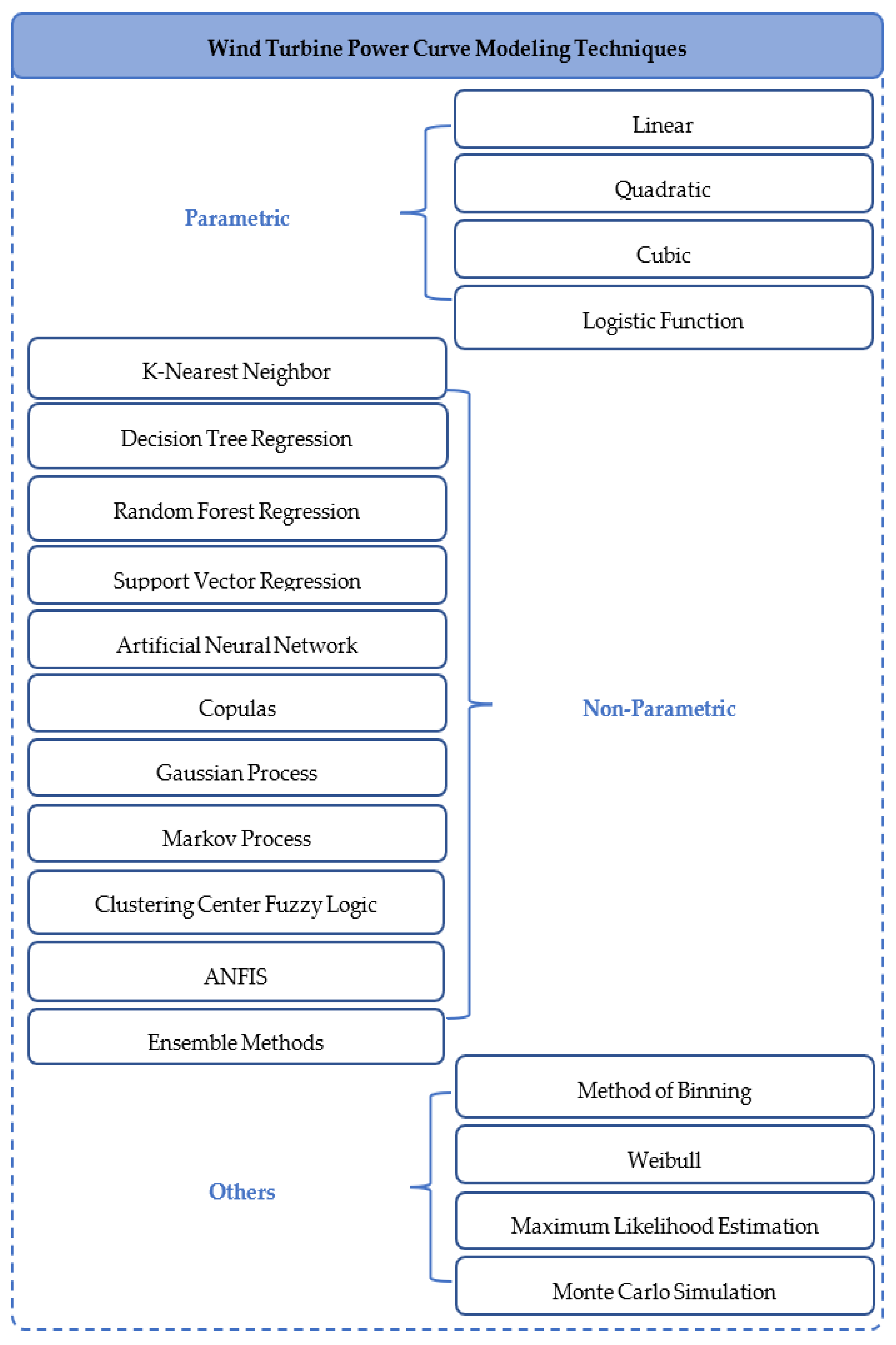
6.1.1. Parametric Algorithms
- (a)
- Linear: The linear model approximates the power curve with a first-degree polynomial. It is indeed the simplest approach to approximate the power curve by a straight line.
- (b)
- Quadratic: The quadratic model approximates the power curve with a second-degree polynomial. In this model, the power curve can be approximated by a slightly curved line.
- (c)
- Cubic: The cubic model approximates the power curve with a third-degree polynomial. In this model, the power curve can be approximated by a further curved line.
- (d)
- Logistic Function: Since the logistic curve is to a certain extent similar to the power curve shape, it can be used to approximate the power curve. For instance, the four-parameters logistic function, can be described as:
6.1.2. Non-Parametric Algorithms
- (a)
- K-Nearest Neighbor (KNN): The “KNN” model is the simplest non-parametric model, which has found success in many applications, including wind turbine power curve modeling. The fundamental principles of the “nearest neighbor” approach is to find a predetermined number of learning samples near (in terms of distance) to the considered sample, and subsequently estimate the label. It is often necessary to define the “number of samples”, which can be a “user-defined” constant “k-nearest neighbor learning” or alter with regards to the local density of points “radius-based neighbor learning”. In general, the distance metric measure is the standard Euclidean distance. According to the reviewed literature, this approach (KNN) is one of the most widely used techniques due to its simplicity. It was employed in [38,44,99,100] for power curve modeling.
- (b)
- Decision Trees Regression (DTR): The “DTR” is essentially a “supervised learning” method which can be used for regression problems such as power curve modeling. It tends to predict the values of a target variable by learning fundamental “decision rules” deduced from the dataset. A so-called “tree” may be considered as a “piecewise constant approximation”. Considering the training data, a “decision tree” employs a recursive partition of the feature space in a way that samples with equivalent targets are gathered. The “quality of a candidate split” of node is calculated through a so-called “impurity function” or “loss function” ,
- (c)
- Random Forest Regression (RFR): The “RFR” is essentially a “meta estimator” which fits several classifying “decision trees” on several subsets of the dataset and employs averaging to enhance the “predictive accuracy” and restrain over-fitting. It is often necessary to specify the number of estimators (trees in the forest) along with the criterion (the function to measure the quality of split), and the maximum depth of the tree. This approach (RFR) was used in [100,101].
- (d)
- Support Vector Regression (SVR): The “SVR” is a model from the family of the “support vector machine” (SVM) used for regression tasks. It is appropriate for modeling from a small-size dataset owing to its powerful ability for generalization. It is often necessary to specify the “kernel” type to be used, for instance, “linear”, “polynomial”, “radial basic function” (RBF), or “sigmoid”. The free parameters for such a model include the “regularization parameter” and “epsilon” which essentially specify the “epsilon-tube” where no “penalty” is syndicated in the learning “loss function” with samples estimated within a distance epsilon from the actual sample. The approximation function is expressed as:
- (e)
- Artificial Neural Network (ANN): The “ANN” is generally comprised of four different parts, namely, the “input layer”, “hidden layers”, “activation function” and “output layer”. The input layer receives the data and transfers to the hidden layers where the information is transformed into higher representation through a nonlinear transformation expressed as , where and denote the vectors of input and hidden representations, respectively, and and represent the weight matrices and bias vectors, respectively. Furthermore, represents the nonlinear activation function; the softmax function calculates the output expressed as:
- (f)
- Copula: The copula model is a probabilistic approach for modeling the wind turbine power curve. Its representation of a power curve may be considered if the power curve is regarded a “bivariate joint distribution”. The function to estimate the copula can be expressed as:
- (g)
- Gaussian Process (GP): The GP model is a “Bayesian non-linear regression” approach widely used to deal with probabilistic regression problems. This approach has also been explored to model the wind turbine power curve. The GP is completely specified by its mean value and covariance function which can be expressed as:
- (h)
- Markov Process (MP): The “MP” is a stochastic model where its condition property demands that the dynamic of the process has no memory, and thus, is solely based on the previous event, and not the entire history. This can be described in terms of its condition probability density function (PDF), expressed as:
- (i)
- Clustering Center Fuzzy Logic (CCFL): The “CCFL” is typically a “fuzzy logic-based” model which has also been explored for modeling the power curve of wind turbine. In this application, datasets are initially clustered and “center of clusters” are established; these “center of clusters” are subsequently employed to represent the power curve of the wind turbine. This approach was used in [44,114,115], where in the prior, the authors found out that, four or five “cluster centers” were sufficient in representing the power curve of wind turbine.
- (j)
- Adaptive Neuro-Fuzzy Interference System (ANFIS): Similar to the “CCFL”, the “ANFIS” is a “fuzzy logic-based” model, which contains a typical fuzzy inference system structure, membership functions, and a set of rules; the approach requires fewer parameters which generally results into a faster training. This approach was used in [44] for power curve modeling purpose.
- (k)
- Ensemble Learning: An ensemble model is an approach of combining different models to improve the overall accuracy to a certain extent which cannot be attained solely by an individual (single) model. Such methods are becoming more and more popular in recent years. An example of such a model can be mathematically expressed as:
6.1.3. Other Algorithms
- (a)
- Method of Binning: The binning method has been already introduced in Section 2.1. It was adopted as the standard by the “international electrotechnical commission” (IEC), and thus, widely used in wind energy technology, for instance by the wind turbine manufacturers for wind turbine certification, and also in academic research. Examples can be found in [100] and in particular in [116] where the power curve reference was attained through the “method of binning”.
- (b)
- Weibull: The “Weibull” is often employed in a typical “probabilistic” power curve estimation model. Assuming that the “wind speed” variable in the dataset follows the “Weibull distribution” with two parameters, the “probability density function” (PDF) for the “wind speed”, , is mathematically described as:
- (c)
- Maximum Likelihood Estimation (MLE): The “MLE” is often used for determination of parameters of power curve models. For instance, in [97] the equations for the “scale and shape parameters” in the “Weibull” wind speed distribution were obtained by maximizing likelihood function, :
- (d)
- Monte Carlo Simulation (MCS): The “MCS” is a probabilistic technique capable of modeling a system under uncertainty. The “Monte Carlo simulation” relies on historical “wind speed” data from wind farm sites. This approach has been used in [117,118]. In particular, it was used in [118] to make a simulation of data in order to complete insufficient real-world dataset and in order to perform analysis in terms of “long-term assessment”.
6.2. Performance Metrics
- (a)
- Mean Absolute Error (MAE): The MAE computes “mean absolute error”, which is a risk metric corresponding to the expected value of the absolute error loss. Assuming that is the actual value and is the predicted value of the th sample, and denotes the number of samples, then the MAE is defined as in Table 8.
- (b)
- Root Mean Squared Error (RMSE): The RMSE is an extension of “mean squared error” (MSE), as the squared root of the error is calculated. MSE computes mean square error, which is a risk metric corresponding to the expected value of the squared (quadratic) error or loss. Assuming that is the actual value and is the predicted value of the th sample, and denotes the number of samples, then the MSE estimated over samples is defined as , hence, the RMSE is defined as in Table 8.
- (c)
- Mean Absolute Percentage Error (MAPE): The MAPE is also known as the “mean absolute percentage deviation” (MAPD). The idea of this metric is to be sensitive to relative errors; it for example does not change by a global scaling of the target variable. Assuming that is the actual value and is the predicted value of the th sample, and denotes the number of samples, then the MAPE is defined as in Table 8.
- (d)
- R-SquaredScore: The R-squared performs the coefficient of determination. It provides an indication of goodness of fit, and therefore, a measure of how well unseen samples are likely to be predicted by the model through the proportion of explained variance. Assuming that is the actual value and is the predicted value of the th sample, and denotes the number of samples; then, is defined as in Table 8.
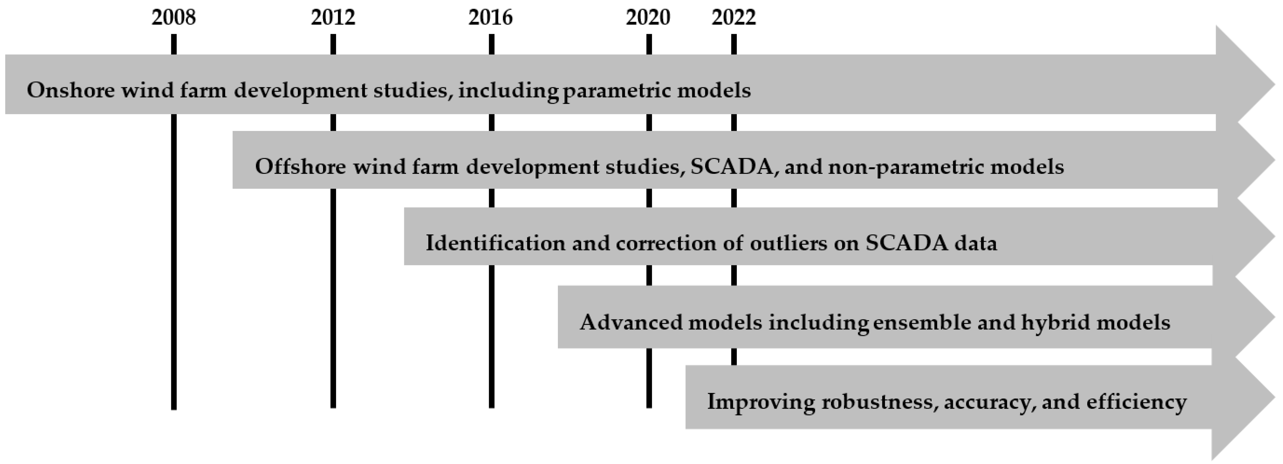
7. Overall Assessment: Past, Present, and Future
8. Discussion and Prospects
- With regards to applications, several key applications of wind turbine power curves, including wind turbine selection, capacity factor estimation, wind energy assessment and forecasting, and condition monitoring, have been discussed in Section 3. According to the reviewed literature, the power curve plays a critical role in wind farm technology, even from the beginnings, when deciding and selecting the characteristics of the wind turbine type to invest in. Capacity factor estimation and wind energy assessment and forecasting provide useful information for operators and wind energy management system; in particular, an accurate implementation of wind energy forecasting can improve services in terms of scheduling and dispatching. Power curve based condition monitoring can provide a general assessment of the entire wind turbine with regards to a wide range of anomaly and fault types, which is very effective for root cause analysis and diagnosis.
- With regards to modeling techniques, a wide range of algorithms, mostly including parametric and non-parametric algorithms, have been explored in Section 6. According to the reviewed literature, most parametric algorithms are based on a typical polynomial expression which is essentially a natural extension of the linear regression (i.e., linear, quadratic, and cubic); a logistic function with four parameters, for instance, is also frequently used. Although they are simple to implement, remarks also indicate that most parametric models do not consider several important factors, hence, they may often result in large errors. Alternatively, non-parametric algorithms including KNN, DTR, RFR, SVR, ANN, Copula, GP, MP, CCFL, ANFIS, and ensemble learning algorithms, among others, are derived from actual wind farm data and mostly attain from the SCADA system; hence, they seem to minimize the prediction error. However, they also are not exempt from limitations; in particular, some non-parametric algorithms can suffer from time-cost due to the required data processing and model training procedures.
- Prospects in this active field is soaring towards robustness; the volatile nature of the wind, not only causes challenges in the utilities and wind energy management system, but also in developing an accurate model. With the recent development of data acquisition systems, researchers are working towards solutions such as multivariate and multi-target models; that is, involving other important condition indicators in addition to the “wind speed” as input variables, and multiple indicators as target variables in addition to “active power”. On another note, the wind energy industry is expanding from onshore to offshore; extensive studies tailored to specific offshore scenarios are expected to appear more frequently. The technology to harvest the wind energy is also improving and advanced wind turbines are being manufactured; hence, there is still room for studies, analysis, and investigations on specific aspects.
9. Conclusions
Author Contributions
Funding
Data Availability Statement
Conflicts of Interest
Nomenclature
| EMS | Energy Management System |
| CMS | Condition Monitoring System |
| SCADA | Supervisory Control and Data Acquisition |
| IEC | International Electrotechnical Commission |
| LCOE | Levelized Cost of Electricity |
| NBMs | Normal Behavior Model |
| LOESS | Locally Weighted Regression |
| DBSCAN | Density-Based Spatial Clustering of Applications with Noise |
| SOM | Self-Organizing Map |
| iForest | Isolation Forest |
| LOF | Local Outlier Factor |
| WCSS | Within Cluster Sum-of-Squares |
| KNN | K-Nearest Neighbor |
| DTR | Decision Tree Regression |
| RFR | Random Forest Regression |
| SVR | Support Vector Regression |
| ANN | Artificial Neural Network |
| GP | Gaussian Process |
| MP | Markov Process |
| CCFL | Clustering Center Fuzzy Logic |
| ANFIS | Adaptive Neuro-Fuzzy Interference System |
| MLE | Maximum Likelihood Estimation |
| MCS | Monte Carlo Simulation |
| Probability Density Function | |
| MAE | Mean Absolute Error |
| RMSE | Root Mean Squared Error |
| MSE | Mean Squared Error |
| MAPE | Mean Absolute Percentage Error |
References
- IRENA. Renewable Power Generation Costs in 2021; International Renewable Energy Agency: Abu Dhabi, United Arab Emirates, 2022. [Google Scholar]
- REN21. Renewables 2022 Global Status Report. In Renewable Energy Policy Network for the 21st Century (REN21); REN21: Paris, France, 2022. [Google Scholar]
- Li, K.; Bian, H.; Liu, C.; Zhang, D.; Yang, Y. Comparison of geothermal with solar and wind power generation systems. Renew. Sustain. Energy Rev. 2015, 42, 1464–1474. [Google Scholar] [CrossRef]
- Shokrzadeh, S.; Jozani, M.J.; Bibeau, E. Wind Turbine Power Curve Modeling Using Advanced Parametric and Nonparametric Methods. IEEE Trans. Sustain. Energy 2014, 5, 1262–1269. [Google Scholar] [CrossRef]
- Tascikaraoglu, A.; Uzunoglu, M. A review of combined approaches for prediction of short-term wind speed and power. Renew. Sustain. Energy Rev. 2014, 34, 243–254. [Google Scholar] [CrossRef]
- Mehrjoo, M.; Jozani, M.J.; Pawlak, M.; Bagen, B. A Multilevel Modeling Approach Towards Wind Farm Aggregated Power Curve. IEEE Trans. Sustain. Energy 2021, 12, 2230–2237. [Google Scholar] [CrossRef]
- Bilendo, F.; Badihi, H.; Lu, N. Wind Turbine Anomaly Detection Based on SCADA Data. Handb. Smart Energy Syst. 2022, 1–24. [Google Scholar] [CrossRef]
- Long, H.; Wang, L.; Zhang, Z.; Song, Z.; Xu, J. Data-Driven Wind Turbine Power Generation Performance Monitoring. IEEE Trans. Ind. Electron. 2015, 62, 6627–6635. [Google Scholar] [CrossRef]
- Cambron, P.; Masson, C.; Tahan, A.; Pelletier, F. Control chart monitoring of wind turbine generators using the statistical inertia of a wind farm average. Renew. Energy 2018, 116, 88–98. [Google Scholar] [CrossRef]
- Helbing, G.; Ritter, M. Improving wind turbine power curve monitoring with standardisation. Renew. Energy 2019, 145, 1040–1048. [Google Scholar] [CrossRef]
- Thapar, V.; Agnihotri, G.; Sethi, V.K. Critical analysis of methods for mathematical modelling of wind turbines. Renew. Energy 2011, 36, 3166–3177. [Google Scholar] [CrossRef]
- Carrillo, C.; Montaño, A.O.; Cidrás, J.; Díaz-Dorado, E. Review of power curve modelling for wind turbines. Renew. Sustain. Energy Rev. 2013, 21, 572–581. [Google Scholar] [CrossRef]
- Lydia, M.; Selvakumar, A.I.; Kumar, S.S.; Kumar, G.E.P. Advanced Algorithms for Wind Turbine Power Curve Modeling. IEEE Trans. Sustain. Energy 2013, 4, 827–835. [Google Scholar] [CrossRef]
- Lydia, M.; Kumar, S.S.; Selvakumar, A.I.; Kumar, G.E.P. A comprehensive review on wind turbine power curve modeling techniques. Renew. Sustain. Energy Rev. 2014, 30, 452–460. [Google Scholar] [CrossRef]
- Yan, J.; Liu, Y.; Han, S.; Wang, Y.; Feng, S. Reviews on uncertainty analysis of wind power forecasting. Renew. Sustain. Energy Rev. 2015, 52, 1322–1330. [Google Scholar] [CrossRef]
- Sohoni, V.; Gupta, S.C.; Nema, R.K. A Critical Review on Wind Turbine Power Curve Modelling Techniques and Their Applications in Wind Based Energy Systems. J. Energy 2016, 2016, 1–18. [Google Scholar] [CrossRef] [Green Version]
- Wang, Y.; Hu, Q.; Li, L.; Foley, A.; Srinivasan, D. Approaches to wind power curve modeling: A review and discussion. Renew. Sustain. Energy Rev. 2019, 116, 109422. [Google Scholar] [CrossRef]
- Lee, G.; Ding, Y.; Xie, L.; Genton, M.G. A kernel plus method for quantifying wind turbine performance upgrades. Wind Energy 2014, 18, 1207–1219. [Google Scholar] [CrossRef]
- Al-Quraan, A.; Al-Masri, H.; Al-Mahmodi, M.; Radaideh, A. Power curve modelling of wind turbines—A comparison study. IET Renew. Power Gener. 2021, 16, 362–374. [Google Scholar] [CrossRef]
- Manobel, B.; Sehnke, F.; Lazzús, J.A.; Salfate, I.; Felder, M.; Montecinos, S. Wind turbine power curve modeling based on Gaussian Processes and Artificial Neural Networks. Renew. Energy 2018, 125, 1015–1020. [Google Scholar] [CrossRef]
- Bilendo, F.; Badihi, H.; Lu, N.; Cambron, P.; Jiang, B. A Normal Behavior Model Based on Power Curve and Stacked Regressions for Condition Monitoring of Wind Turbines. IEEE Trans. Instrum. Meas. 2022, 71, 1–13. [Google Scholar] [CrossRef]
- Stanley, A.P.; Roberts, O.; Lopez, A.; Williams, T.; Barker, A. Turbine scale and siting considerations in wind plant layout optimization and implications for capacity density. Energy Rep. 2022, 8, 3507–3525. [Google Scholar] [CrossRef]
- Hu, S.-Y.; Cheng, J.-H. Performance evaluation of pairing between sites and wind turbines. Renew. Energy 2007, 32, 1934–1947. [Google Scholar] [CrossRef]
- Liu, Y.; Fu, Y.; Huang, L.-L.; Zhang, K. Reborn and upgrading: Optimum repowering planning for offshore wind farms. Energy Rep. 2022, 8, 5204–5214. [Google Scholar] [CrossRef]
- Pallabazzer, R. Parametric analysis of wind siting efficiency. J. Wind. Eng. Ind. Aerodyn. 2003, 91, 1329–1352. [Google Scholar] [CrossRef]
- Song, D.; Yang, Y.; Zheng, S.; Tang, W.; Yang, J.; Su, M.; Yang, X.; Joo, Y.H. Capacity factor estimation of variable-speed wind turbines considering the coupled influence of the QN-curve and the air density. Energy 2019, 183, 1049–1060. [Google Scholar] [CrossRef]
- Albadi, M.H.; El-Saadany, E.F. Wind Turbines Capacity Factor Modeling—A Novel Approach. IEEE Trans. Power Syst. 2009, 24, 1637–1638. [Google Scholar] [CrossRef]
- Ayodele, T.; Jimoh, A.; Munda, J.; Agee, J. Wind distribution and capacity factor estimation for wind turbines in the coastal region of South Africa. Energy Convers. Manag. 2012, 64, 614–625. [Google Scholar] [CrossRef]
- Ditkovich, Y.; Kuperman, A.; Yahalom, A.; Byalsky, M. A Generalized Approach to Estimating Capacity Factor of Fixed Speed Wind Turbines. IEEE Trans. Sustain. Energy 2012, 3, 607–608. [Google Scholar] [CrossRef]
- Yeh, T.-H.; Wang, L. A Study on Generator Capacity for Wind Turbines Under Various Tower Heights and Rated Wind Speeds Using Weibull Distribution. IEEE Trans. Energy Convers. 2008, 23, 592–602. [Google Scholar] [CrossRef]
- Souloukngaa, M.H.; Coban, H.H. Determination of Feasibility Analysis of Wind Turbines Using Weibull Parameter for Chad. J. Smart Sci. Technol. 2022, 2, 1–15. [Google Scholar] [CrossRef]
- Zeng, J.; Qiao, W. Short-Term Wind Power Prediction Using a Wavelet Support Vector Machine. IEEE Trans. Sustain. Energy 2012, 3, 255–264. [Google Scholar] [CrossRef]
- Faulstich, S.; Hahn, B.; Tavner, P.J. Wind turbine downtime and its importance for offshore deployment. Wind Energy 2011, 14, 327–337. [Google Scholar] [CrossRef]
- Carroll, J.; McDonald, A.; McMillan, D. Failure rate, repair time and unscheduled O&M cost analysis of offshore wind turbines. Wind Energy 2016, 19, 1107–1119. [Google Scholar] [CrossRef] [Green Version]
- Pfaffel, S.; Faulstich, S.; Rohrig, K. Performance and Reliability of Wind Turbines: A Review. Energies 2017, 10, 1904. [Google Scholar] [CrossRef] [Green Version]
- Garcia Márquez, F.P.; Tobias, A.M.; Pérez, J.M.P.; Papaelias, M. Condition monitoring of wind turbines: Techniques and methods. Renew. Energy 2012, 46, 169–178. [Google Scholar] [CrossRef]
- Zaher, A.; McArthur, S.; Infield, D.; Patel, Y. Online wind turbine fault detection through automated SCADA data analysis. Wind. Energy 2009, 12, 574–593. [Google Scholar] [CrossRef]
- Kusiak, A.; Zheng, H.; Song, Z. On-line monitoring of power curves. Renew. Energy 2009, 34, 1487–1493. [Google Scholar] [CrossRef]
- Kusiak, A.; Li, W. The prediction and diagnosis of wind turbine faults. Renew. Energy 2011, 36, 16–23. [Google Scholar] [CrossRef]
- Schlechtingen, M.; Santos, I.F.; Achiche, S. Wind turbine condition monitoring based on SCADA data using normal behavior models. Part 1: System description. Appl. Soft Comput. 2013, 13, 259–270. [Google Scholar] [CrossRef]
- Tautz-Weinert, J.; Watson, S. Using SCADA data for wind turbine condition monitoring—A review. IET Renew. Power Gener. 2016, 11, 382–394. [Google Scholar] [CrossRef] [Green Version]
- Maldonado-Correa, J.; Martín-Martínez, S.; Artigao, E.; Gómez-Lázaro, E. Using SCADA Data for Wind Turbine Condition Monitoring: A Systematic Literature Review. Energies 2020, 13, 3132. [Google Scholar] [CrossRef]
- Marvuglia, A.; Messineo, A. Monitoring of wind farms’ power curves using machine learning techniques. Appl. Energy 2012, 98, 574–583. [Google Scholar] [CrossRef]
- Schlechtingen, M.; Santos, I.F.; Achiche, S. Using Data-Mining Approaches for Wind Turbine Power Curve Monitoring: A Comparative Study. IEEE Trans. Sustain. Energy 2013, 4, 671–679. [Google Scholar] [CrossRef]
- Schlechtingen, M.; Santos, I.F. Wind turbine condition monitoring based on SCADA data using normal behavior models. Part 2: Application examples. Appl. Soft Comput. 2014, 14, 447–460. [Google Scholar] [CrossRef]
- Meyer, A.; Brodbeck, B. Data-driven Performance Fault Detection in Commercial Wind Turbines. In Proceedings of the 5th European Conference of the Prognostics and Health Management Society (PHME20), Turin, Italy, 1–3 July 2020. [Google Scholar]
- Meyer, A. Multi-target normal behaviour models for wind farm condition monitoring. Appl. Energy 2021, 300, 117342. [Google Scholar] [CrossRef]
- Stetco, A.; Dinmohammadi, F.; Zhao, X.; Robu, V.; Flynn, D.; Barnes, M.; Keane, J.; Nenadic, G. Machine learning methods for wind turbine condition monitoring: A review. Renew. Energy 2019, 133, 620–635. [Google Scholar] [CrossRef]
- Helbing, G.; Ritter, M. Deep Learning for fault detection in wind turbines. Renew. Sustain. Energy Rev. 2018, 98, 189–198. [Google Scholar] [CrossRef]
- Meyer, A. Early Fault Detection with Multi-target Neural Networks. In Computational Science and Its Applications—ICCSA 2021; Lecture Notes in Computer Science; Gervasi, O., Ed.; Springer: Berlin/Heidelberg, Germany, 2021; Volume 12951. [Google Scholar]
- Li, Y.; Liu, S.; Shu, L. Wind turbine fault diagnosis based on Gaussian process classifiers applied to operational data. Renew. Energy 2018, 134, 357–366. [Google Scholar] [CrossRef]
- Xu, Q.; Fan, Z.; Jia, W.; Jiang, C. Fault detection of wind turbines via multivariate process monitoring based on vine copulas. Renew. Energy 2020, 161, 939–955. [Google Scholar] [CrossRef]
- Aziz, U.; Charbonnier, S.; Bérenguer, C.; Lebranchu, A.; Prevost, F. Critical comparison of power-based wind turbine fault-detection methods using a realistic framework for SCADA data simulation. Renew. Sustain. Energy Rev. 2021, 144, 110961. [Google Scholar] [CrossRef]
- Badihi, H.; Zhang, Y.; Jiang, B.; Pillay, P.; Rakheja, S. A Comprehensive Review on Signal-Based and Model-Based Condition Monitoring of Wind Turbines: Fault Diagnosis and Lifetime Prognosis. Proc. IEEE 2022, 110, 754–806. [Google Scholar] [CrossRef]
- Gill, S.; Stephen, B.; Galloway, S. Wind Turbine Condition Assessment Through Power Curve Copula Modeling. IEEE Trans. Sustain. Energy 2011, 3, 94–101. [Google Scholar] [CrossRef] [Green Version]
- Shen, X.; Fu, X.; Zhou, C. A Combined Algorithm for Cleaning Abnormal Data of Wind Turbine Power Curve Based on Change Point Grouping Algorithm and Quartile Algorithm. IEEE Trans. Sustain. Energy 2018, 10, 46–54. [Google Scholar] [CrossRef]
- Badihi, H.; Zhang, Y.; Pillay, P.; Rakheja, S. Fault-Tolerant Individual Pitch Control for Load Mitigation in Wind Turbines with Actuator Faults. IEEE Trans. Ind. Electron. 2020, 68, 532–543. [Google Scholar] [CrossRef]
- Badihi, H.; Jadidi, S.; Zhang, Y.; Pillay, P.; Rakheja, S. Fault-Tolerant Cooperative Control in a Wind Farm Using Adaptive Control Reconfiguration and Control Reallocation. IEEE Trans. Sustain. Energy 2019, 11, 2119–2129. [Google Scholar] [CrossRef]
- Park, J.-Y.; Lee, J.-K.; Oh, K.-Y.; Lee, J.-S. Development of a Novel Power Curve Monitoring Method for Wind Turbines and Its Field Tests. IEEE Trans. Energy Convers. 2014, 29, 119–128. [Google Scholar] [CrossRef]
- Ye, X.; Lu, Z.; Qiao, Y.; Min, Y.; O’Malley, M. Identification and Correction of Outliers in Wind Farm Time Series Power Data. IEEE Trans. Power Syst. 2016, 31, 4197–4205. [Google Scholar] [CrossRef]
- Yesilbudak, M. Implementation of novel hybrid approaches for power curve modeling of wind turbines. Energy Convers. Manag. 2018, 171, 156–169. [Google Scholar] [CrossRef]
- Yuan, T.; Sun, Z.; Ma, S. Gearbox Fault Prediction of Wind Turbines Based on a Stacking Model and Change-Point Detection. Energies 2019, 12, 4224. [Google Scholar] [CrossRef] [Green Version]
- Long, H.; Sang, L.; Wu, Z.; Gu, W. Image-Based Abnormal Data Detection and Cleaning Algorithm via Wind Power Curve. IEEE Trans. Sustain. Energy 2019, 11, 938–946. [Google Scholar] [CrossRef]
- Han, S.; Qiao, Y.; Yan, P.; Yan, J.; Liu, Y.; Li, L. Wind turbine power curve modeling based on interval extreme probability density for the integration of renewable energies and electric vehicles. Renew. Energy 2020, 157, 190–203. [Google Scholar] [CrossRef]
- Zhang, S.; Lang, Z.-Q. SCADA-data-based wind turbine fault detection: A dynamic model sensor method. Control. Eng. Pract. 2020, 102, 104546. [Google Scholar] [CrossRef]
- Moreno, S.R.; Coelho, L.D.S.; Ayala, H.V.; Mariani, V.C. Wind turbines anomaly detection based on power curves and ensemble learning. IET Renew. Power Gener. 2020, 14, 4086–4093. [Google Scholar] [CrossRef]
- Wang, Y.; Hu, Q.; Pei, S. Wind Power Curve Modeling with Asymmetric Error Distribution. IEEE Trans. Sustain. Energy 2019, 11, 1199–1209. [Google Scholar] [CrossRef]
- Liang, G.; Su, Y.; Chen, F.; Long, H.; Song, Z.; Gan, Y. Wind Power Curve Data Cleaning by Image Thresholding Based on Class Uncertainty and Shape Dissimilarity. IEEE Trans. Sustain. Energy 2020, 12, 1383–1393. [Google Scholar] [CrossRef]
- Morrison, R.; Liu, X.; Lin, Z. Anomaly detection in wind turbine SCADA data for power curve cleaning. Renew. Energy 2022, 184, 473–486. [Google Scholar] [CrossRef]
- Bilendo, F.; Badihi, H.; Lu, N.; Cambron, P.; Jiang, B. Power Curve-Based Fault Detection Method for Wind Turbines. Ifac-Papersonline 2022, 55, 408–413. [Google Scholar] [CrossRef]
- Zeng, X.; Yang, M.; Bo, Y. Gearbox oil temperature anomaly detection for wind turbine based on sparse Bayesian probability estimation. Int. J. Electr. Power Energy Syst. 2020, 123, 106233. [Google Scholar] [CrossRef]
- Duong, B.P.; Khan, S.A.; Shon, D.; Im, K.; Park, J.; Lim, D.-S.; Jang, B.; Kim, J.-M. A Reliable Health Indicator for Fault Prognosis of Bearings. Sensors 2018, 18, 3740. [Google Scholar] [CrossRef] [Green Version]
- Kusiak, A.; Verma, A. Monitoring Wind Farms with Performance Curves. IEEE Trans. Sustain. Energy 2012, 4, 192–199. [Google Scholar] [CrossRef]
- Yan, J.; Zhang, H.; Liu, Y.; Han, S.; Li, L. Uncertainty estimation for wind energy conversion by probabilistic wind turbine power curve modelling. Appl. Energy 2019, 239, 1356–1370. [Google Scholar] [CrossRef]
- Zhao, Y.; Ye, L.; Wang, W.; Sun, H.; Ju, Y.; Tang, Y. Data-Driven Correction Approach to Refine Power Curve of Wind Farm Under Wind Curtailment. IEEE Trans. Sustain. Energy 2017, 9, 95–105. [Google Scholar] [CrossRef]
- Souza, L.G.M.; Santos, D.C. A Performance Comparison of Robust Models in Wind Turbines Power Curve Estimation: A Case Study. Neural Process. Lett. 2022, 54, 3375–3400. [Google Scholar] [CrossRef]
- Bilendo, F.; Badihi, H.; Lu, N.; Cambron, P.; Jiang, B. Imaging Wind Turbine Fault Signatures Based on Power Curve and Self-Organizing Map for Image-Based Fault Diagnosis. In Proceedings of the 2022 IEEE International Symposium on Advanced Control of Industrial Processes, Vancouver, BC, Canada, 7–9 August 2022; pp. 204–209. [Google Scholar] [CrossRef]
- Wang, Y.; Infield, D.G.; Stephen, B.; Galloway, S.J. Copula-based model for wind turbine power curve outlier rejection. Wind Energy 2013, 17, 1677–1688. [Google Scholar] [CrossRef] [Green Version]
- Li, T.; Liu, X.; Lin, Z.; Morrison, R. Ensemble offshore Wind Turbine Power Curve modelling—An integration of Isolation Forest, fast Radial Basis Function Neural Network, and metaheuristic algorithm. Energy 2022, 239. [Google Scholar] [CrossRef]
- Zheng, L.; Hu, W.; Min, Y. Raw Wind Data Preprocessing: A Data-Mining Approach. IEEE Trans. Sustain. Energy 2014, 6, 11–19. [Google Scholar] [CrossRef]
- Sainz, E.; Llombart, A.; Guerrero, J. Robust filtering for the characterization of wind turbines: Improving its operation and maintenance. Energy Convers. Manag. 2009, 50, 2136–2147. [Google Scholar] [CrossRef]
- Bangalore, P.; Letzgus, S.; Karlsson, D.; Patriksson, M. An artificial neural network-based condition monitoring method for wind turbines, with application to the monitoring of the gearbox. Wind Energy 2017, 20, 1421–1438. [Google Scholar] [CrossRef]
- Zhao, Y.; Li, D.; Dong, A.; Kang, D.; Lv, Q.; Shang, L. Fault Prediction and Diagnosis of Wind Turbine Generators Using SCADA Data. Energies 2017, 10, 1210. [Google Scholar] [CrossRef] [Green Version]
- Javadi, M.; Malyscheff, A.M.; Wu, D.; Kang, C.; Jiang, J.N. An algorithm for practical power curve estimation of wind turbines. CSEE J. Power Energy Syst. 2018, 4, 93–102. [Google Scholar] [CrossRef]
- Teng, W.; Cheng, H.; Ding, X.; Liu, Y.; Ma, Z.; Mu, H. DNN-based approach for fault detection in a direct drive wind turbine. IET Renew. Power Gener. 2018, 12, 1164–1171. [Google Scholar] [CrossRef]
- Hu, Y.; Qiao, Y.; Liu, J.-Z.; Zhu, H. Adaptive Confidence Boundary Modeling of Wind Turbine Power Curve Using SCADA Data and Its Application. IEEE Trans. Sustain. Energy 2018, 10, 1330–1341. [Google Scholar] [CrossRef]
- Hu, Y.; Xi, Y.; Pan, C.; Li, G.; Chen, B. Daily condition monitoring of grid-connected wind turbine via high-fidelity power curve and its comprehensive rating. Renew. Energy 2020, 146, 2095–2111. [Google Scholar] [CrossRef]
- Trizoglou, P.; Liu, X.; Lin, Z. Fault detection by an ensemble framework of Extreme Gradient Boosting (XGBoost) in the operation of offshore wind turbines. Renew. Energy 2021, 179, 945–962. [Google Scholar] [CrossRef]
- Xiang, L.; Yang, X.; Hu, A.; Su, H.; Wang, P. Condition monitoring and anomaly detection of wind turbine based on cascaded and bidirectional deep learning networks. Appl. Energy 2021, 305, 117925. [Google Scholar] [CrossRef]
- Yao, Q.; Hu, Y.; Liu, J.; Zhao, T.; Qi, X.; Sun, S. Power Curve Modeling for Wind Turbine using Hybrid-Driven Outlier Detection Method. J. Mod. Power Syst. Clean Energy 2022, 1–11. [Google Scholar]
- Luo, Z.; Fang, C.; Liu, C.; Liu, S. Method for Cleaning Abnormal Data of Wind Turbine Power Curve Based on Density Clustering and Boundary Extraction. IEEE Trans. Sustain. Energy 2021, 13, 1147–1159. [Google Scholar] [CrossRef]
- Mehrjoo, M.; Jozani, M.J.; Pawlak, M. Wind turbine power curve modeling for reliable power prediction using monotonic regression. Renew. Energy 2019, 147, 214–222. [Google Scholar] [CrossRef]
- Taslimi-Renani, E.; Modiri-Delshad, M.; Elias, M.F.M.; Rahim, N.A. Development of an enhanced parametric model for wind turbine power curve. Appl. Energy 2016, 177, 544–552. [Google Scholar] [CrossRef]
- Chen, J.; Wang, F.; Stelson, K.A. A mathematical approach to minimizing the cost of energy for large utility wind turbines. Appl. Energy 2018, 228, 1413–1422. [Google Scholar] [CrossRef]
- Chang, T.-P.; Liu, F.-J.; Ko, H.-H.; Cheng, S.-P.; Sun, L.-C.; Kuo, S.-C. Comparative analysis on power curve models of wind turbine generator in estimating capacity factor. Energy 2014, 73, 88–95. [Google Scholar] [CrossRef]
- Liu, X. An Improved Interpolation Method for Wind Power Curves. IEEE Trans. Sustain. Energy 2012, 3, 528–534. [Google Scholar] [CrossRef]
- Seo, S.; Oh, S.-D.; Kwak, H.-Y. Wind turbine power curve modeling using maximum likelihood estimation method. Renew. Energy 2018, 136, 1164–1169. [Google Scholar] [CrossRef]
- Villanueva, D.; Feijóo, A.E. Reformulation of parameters of the logistic function applied to power curves of wind turbines. Electr. Power Syst. Res. 2016, 137, 51–58. [Google Scholar] [CrossRef]
- Kusiak, A.; Zheng, H.; Song, Z. Models for monitoring wind farm power. Renew. Energy 2009, 34, 583–590. [Google Scholar] [CrossRef]
- Janssens, O.; Noppe, N.; Devriendt, C.; Van de Walle, R.; Van Hoecke, S. Data-driven multivariate power curve modeling of offshore wind turbines. Eng. Appl. Artif. Intell. 2016, 55, 331–338. [Google Scholar] [CrossRef]
- Pandit, R.K.; Infield, D.; Kolios, A. Comparison of advanced non-parametric models for wind turbine power curves. IET Renew. Power Gener. 2019, 13, 1503–1510. [Google Scholar] [CrossRef] [Green Version]
- Ouyang, T.; Kusiak, A.; He, Y. Modeling wind-turbine power curve: A data partitioning and mining approach. Renew. Energy 2017, 102, 1–8. [Google Scholar] [CrossRef]
- Pelletier, F.; Masson, C.; Tahan, A. Wind turbine power curve modelling using artificial neural network. Renew. Energy 2016, 89, 207–214. [Google Scholar] [CrossRef]
- Stephen, B.; Galloway, S.J.; McMillan, D.; Hill, D.C.; Infield, D.G. A Copula Model of Wind Turbine Performance. IEEE Trans. Power Syst. 2010, 26, 965–966. [Google Scholar] [CrossRef] [Green Version]
- Wei, D.; Wang, J.; Li, Z.; Wang, R. Wind Power Curve Modeling with Hybrid Copula and Grey Wolf Optimization. IEEE Trans. Sustain. Energy 2021, 13, 265–276. [Google Scholar] [CrossRef]
- Pandit, R.K.; Infield, D. SCADA-based wind turbine anomaly detection using Gaussian process models for wind turbine condition monitoring purposes. IET Renew. Power Gener. 2018, 12, 1249–1255. [Google Scholar] [CrossRef] [Green Version]
- Pandit, R.K.; Infield, D. Comparative analysis of Gaussian Process power curve models based on different stationary covariance functions for the purpose of improving model accuracy. Renew. Energy 2019, 140, 190–202. [Google Scholar] [CrossRef] [Green Version]
- Pandit, R.; Infield, D.; Kolios, A. Gaussian process power curve models incorporating wind turbine operational variables. Energy Rep. 2020, 6, 1658–1669. [Google Scholar] [CrossRef]
- Virgolino, G.C.; Mattos, C.L.; Magalhães, J.A.F.; Barreto, G.A. Gaussian processes with logistic mean function for modeling wind turbine power curves. Renew. Energy 2020, 162, 458–465. [Google Scholar] [CrossRef]
- Guo, P.; Infield, D. Wind Turbine Power Curve Modeling and Monitoring with Gaussian Process and SPRT. IEEE Trans. Sustain. Energy 2018, 11, 107–115. [Google Scholar] [CrossRef] [Green Version]
- Rogers, T.; Gardner, P.; Dervilis, N.; Worden, K.; Maguire, A.; Papatheou, E.; Cross, E. Probabilistic modelling of wind turbine power curves with application of heteroscedastic Gaussian Process regression. Renew. Energy 2020, 148, 1124–1136. [Google Scholar] [CrossRef]
- Bull, L.; Gardner, P.; Rogers, T.; Dervilis, N.; Cross, E.; Papatheou, E.; Maguire, A.; Campos, C.; Worden, K. Bayesian modelling of multivalued power curves from an operational wind farm. Mech. Syst. Signal Process. 2021, 169, 108530. [Google Scholar] [CrossRef]
- Anahua, E.; Barth, S.; Peinke, J. Markovian power curves for wind turbines. Wind Energy 2007, 11, 219–232. [Google Scholar] [CrossRef]
- Ustuntas, T.; Şahin, A.D. Wind turbine power curve estimation based on cluster center fuzzy logic modeling. J. Wind Eng. Ind. Aerodyn. 2008, 96, 611–620. [Google Scholar] [CrossRef]
- De la Hermosa González, R.R. Wind farm monitoring using Mahalanobis distance and fuzzy clustering. Renew. Energy 2018, 123, 526–540. [Google Scholar] [CrossRef]
- Cambron, P.; Lepvrier, R.; Masson, C.; Tahan, A.; Pelletier, F. Power curve monitoring using weighted moving average control charts. Renew. Energy 2016, 94, 126–135. [Google Scholar] [CrossRef]
- Yun, E.; Hur, J. Probabilistic estimation model of power curve to enhance power output forecasting of wind generating resources. Energy 2021, 223, 120000. [Google Scholar] [CrossRef]
- Villanueva, D.; Feijoo, A. Normal-Based Model for True Power Curves of Wind Turbines. IEEE Trans. Sustain. Energy 2016, 7, 1005–1011. [Google Scholar] [CrossRef]
- Albadi, M.; El-Saadany, E. Optimum turbine-site matching. Energy 2010, 35, 3593–3602. [Google Scholar] [CrossRef]
- Marčiukaitis, M.; Žutautaitė, I.; Martišauskas, L.; Jokšas, B.; Gecevičius, G.; Sfetsos, A. Non-linear regression model for wind turbine power curve. Renew. Energy 2017, 113, 732–741. [Google Scholar] [CrossRef]
- You, M.; Liu, B.; Byon, E.; Huang, S.; Jin, J. Direction-Dependent Power Curve Modeling for Multiple Interacting Wind Turbines. IEEE Trans. Power Syst. 2017, 33, 1725–1733. [Google Scholar] [CrossRef]
- Wang, Y.; Hu, Q.; Srinivasan, D.; Wang, Z. Wind Power Curve Modeling and Wind Power Forecasting with Inconsistent Data. IEEE Trans. Sustain. Energy 2018, 10, 16–25. [Google Scholar] [CrossRef]
- Saint-Drenan, Y.-M.; Besseau, R.; Jansen, M.; Staffell, I.; Troccoli, A.; Dubus, L.; Schmidt, J.; Gruber, K.; Simoes, S.; Heier, S. A parametric model for wind turbine power curves incorporating environmental conditions. Renew. Energy 2020, 157, 754–768. [Google Scholar] [CrossRef]
- Karamichailidou, D.; Kaloutsa, V.; Alexandridis, A. Wind turbine power curve modeling using radial basis function neural networks and tabu search. Renew. Energy 2020, 163, 2137–2152. [Google Scholar] [CrossRef]
- Xu, K.; Yan, J.; Zhang, H.; Zhang, H.; Han, S.; Liu, Y. Quantile based probabilistic wind turbine power curve model. Appl. Energy 2021, 296, 116913. [Google Scholar] [CrossRef]
- Zou, R.; Yang, J.; Wang, Y.; Liu, F.; Essaaidi, M.; Srinivasan, D. Wind turbine power curve modeling using an asymmetric error characteristic-based loss function and a hybrid intelligent optimizer. Appl. Energy 2021, 304, 117707. [Google Scholar] [CrossRef]
- Wang, Y.; Li, Y.; Zou, R.; Foley, A.M.; Al Kez, D.; Song, D.; Hu, Q.; Srinivasan, D. Sparse Heteroscedastic Multiple Spline Regression Models for Wind Turbine Power Curve Modeling. IEEE Trans. Sustain. Energy 2020, 12, 191–201. [Google Scholar] [CrossRef]
- Yang, L.; Wang, L.; Zhang, Z. Generative Wind Power Curve Modeling Via Machine Vision: A Deep Convolutional Network Method with Data-Synthesis-Informed-Training. IEEE Trans. Power Syst. 2022, 1. [Google Scholar] [CrossRef]
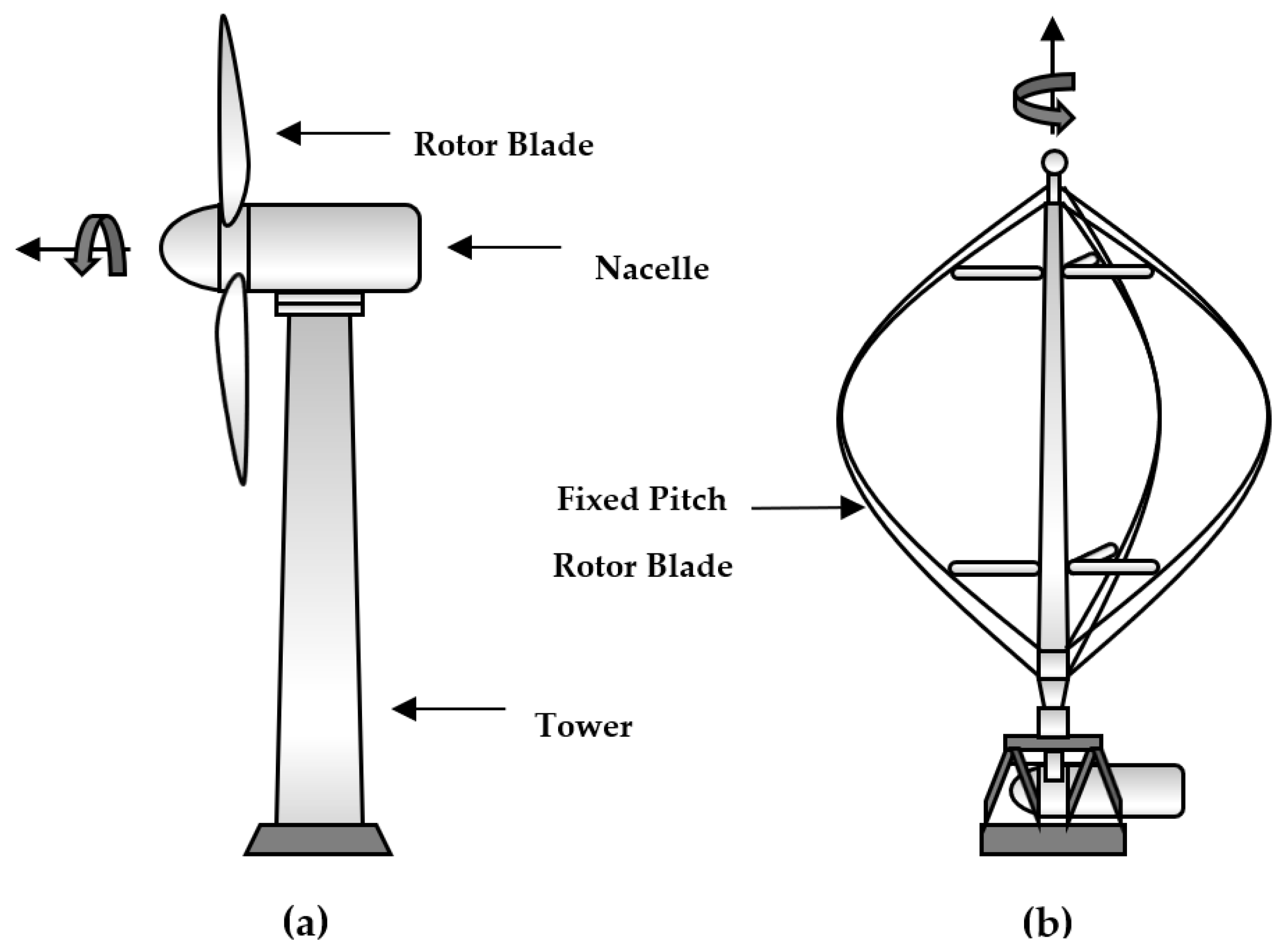
- Breeze, P. (Ed.) The Anatomy of a Wind Turbine. In Wind Power Generation; Academic Press: Cambridge, MA, USA, 2016; pp. 19–27. [Google Scholar]


| Ref. | Author(s) and Year | Brief Description |
|---|---|---|
| [11] | (Thapar, et al., 2011) | A critical analysis on “mathematical modelling” methods for power curve. |
| [12] | (Carrillo, et al., 2013) | A review on the equations for power curve modeling; the “polynomial, exponential, and cubic”. |
| [13] | (Lydia, et al., 2013) | An overview on several “parametric” and “non-parametric” algorithms for power curve modeling. |
| [5] | (Tascikaraoglu & Uzunoglu, 2014) | A review on combined methods for wind power forecasting. |
| [14] | (Lydia, et al., 2014) | A review on the parametric and nonparametric techniques for power curve modeling. |
| [15] | (Yan, et al., 2015) | A review on “uncertainty analysis” of wind power forecasting; a probabilistic approach. |
| [16] | (Sohoni, et al., 2016) | A critical overview on power curve modelling techniques and applications for wind turbines. |
| [17] | (Wang, et al., 2019) | An overview on power curve modelling; analysis in distinct seasons, including wind farms. |
| Types | Anomaly and Fault Description [21] |
|---|---|
| Type 1 | Lower Stacked Data: In such events, anomalous and fault signature can be identified through the “lower-horizontal data”, in which the assigned power value is relatively equal to zero, including in situations where the wind speed is above the “rated wind speed”. Root cause: according to the reviewed literature, such events are typically caused due to “damaged power measuring instrument”, or “communication equipment fault”. |
| Type 2 | Down-Rating: Also known as “Power Curtailment or Derated”, such events are identifiable by its signature in “the middle-horizontal data”; in those situations, the power curve stays mostly constant at a specified rate and no changes are made with regards to wind speed. Root cause 1: according to the reviewed literature, down-rating may occur due to an imposed “control action”, to restrict power production to a level below its maximum efficiency. Reasons for activation of such action, includes the excess capacity of wind power with no substantial resources for storing; also, the wind speed instability, in particular “huge fluctuations”, can play a role. Root cause 2: Alternatively, such events may also be caused by “load sensor failure”. |
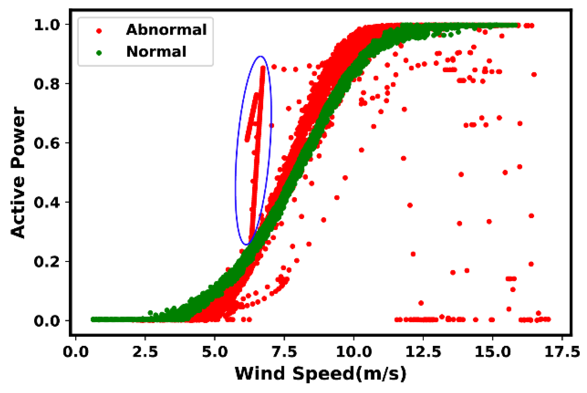
| Type 3 | Wind Speed Under-Reading: The “stacked-vertical data” beyond the power curve reference, in situations where there is an increase in power value, but not necessarily in regard to wind speed, can often be an indication of such event. Root-cause(s): There may be a variety of reasons that may trigger such events, for instance “wind speed sensor malfunction/failure”, “communication equipment error”, and/or “power measuring instrument failure”. However, to the best of author’s knowledge, specific details on this regard have not been broadly reported. |
| Type 4 | Dispersive (Spread) Data: It refers to the “randomly distributed data points” all around the curve. Root cause 1: According to the reviewed literature, the “turbulence produced by the wake effects” or “wind turbine loading ramp” that occurs while starting or stopping the wind turbine, are reportedly some of the root-causes. Root cause 2: Alternatively, it may be caused by “sensor accuracy degradation”, “instrument fault”, and “noise during signal processing by the system”. |
| Type 5 | Icing/Debris Build-up on Blades: The shift of a cluster of data points when compared with the reference power curve, often indicates events such as icing and/or debris build-up on blades. Root cause: Such events are mostly dependent on the environmental conditions and geographic location of the wind farm. |
| Ref. | Author(s) and Year | Brief Description |
|---|---|---|
| [43] | (Marvuglia & Messineo, 2012) | A discussion on the presence of outliers and abnormal values on power curve, including root-causes. |
| [55] | (Gill, et al., 2012) | A discussion on three “fault modes” that provide a subdivision of all possible faults. |
| [59] | (Park, et al., 2014) | Visual illustration of seven types of power curve deviations, and the related anomaly or fault types. |
| [60] | (Ye, et al., 2016) | Addressing four types of anomaly and fault types, including the root-causes. |
| [61] | (Yesilbudak, 2018) | Addressing several root-causes that cause different types of anomaly and fault types on power curve. |
| [62] | (Yuan, et al., 2019) | A discussion on three common anomaly and fault types on power curve. |
| [56] | (Shen, et al., 2019) | Addressing four types of anomaly and fault, according to the data distribution characteristics. |
| [63] | (Long, et al., 2020) | A brief discussion on three common anomaly and fault types. |
| [64] | (Han, et al., 2020) | Addressing three common anomaly and fault types on power curve, including root-causes. |
| [65] | (Zhang & Lang, 2020) | A brief discussion on power curve-based curtailment outliers in the SCADA data. |
| [66] | (Moreno, et al., 2020) | Addressing three modes of degradation through power curve. |
| [67] | (Wang, et al., 2020) | Briefly addressing and illustrating three types of reprehensive outliers on power curve. |
| [68] | (Liang, et al., 2021) | Briefly addressing three categories of abnormal data on wind turbine power curve. |
| [21] | (Bilendo, et al., 2022) | Addressing five types of most common anomalies and faults on power curve, including root-causes. |
| [69] | (Morrison, et al., 2022) | Briefly addressing three common anomaly and fault types on power curve. |
| Method | Essential Parameters | Advantages and Limitations (Pros and Cons) |
|---|---|---|
| Moving Mean | The moving window size | Pros: The method is simple and easy to implement. Cons: A large size moving window can lead to loss of information. |
| LOESS | The span size | Pros: The method is simple and easy to implement. Cons: A large span value can lead to loss of information. |
| K-Means Clustering | Number of clusters | Pros: The method is simple and easy to implement. Cons: It is challenging to attain an optimal number of clusters. |
| DBSCAN | Maximum distance; Number of samples in neighborhood; Distance metric | Pros: The model does not require specification of number of clusters. Cons: May suffer from time-cost when used on large-size datasets. |
| Self-Organizing Map | Grid size; Neighborhood radius; Learning rate | Pros: The method enables time-series and image-based approaches. Cons: Difficult to determine input weights. |
| Isolation Forest | Number of estimators; Contamination | Pros: Works well on small sample size, but also capable of rescaling. Cons: The model can suffer from bias. |
| Local Outlier Factor | Number of neighbors; Distance metric; Contamination | Pros: The model is density-based. Cons: Challenging to understand the decisions based on score. |
| Combined Methods | Depends on the constituents; | Pros: Such method may attain better result compared to single-based. Cons: May suffer from time-cost depending on its complexity. |
| Ref. | Author(s) and Year | Brief Description |
|---|---|---|
| [81] | (Sainz, et al., 2009) | A robust statistical filtering method based on “Least Median Squares” combined with random search. |
| [73] | (Kusiak & Verma, 2013) | A multivariate approach for outlier detection based on “k-means clustering” and “Mahalanobis distance”. |
| [59] | (Park, et al., 2014) | An algorithm for power curve modeling, which automatically calculates the power curve limits. |
| [78] | (Wang, et al., 2014) | A data clustering procedure based on SOM. |
| [80] | (Zheng, et al., 2015) | Data preprocessing and filtering approach involving LOF. |
| [60] | (Ye, et al., 2016) | Outlier detection and correction method. |
| [82] | (Bangalore, et al., 2017) | A methodology for data preprocessing and post-processing including anomaly detection. |
| [83] | (Zhao, et al., 2017) | SCADA data processing including a data cleaning procedure for diagnosis and prognosis purposes. |
| [20] | (Manobel, et al., 2018) | An automatic filtering, by means of Gaussian Process, is employed prior to modeling through ANN. |
| [61] | (Yesilbudak, 2018) | “Clustering, filtering and modeling”; using the “k-means-based Smoothing Spline hybrid” model. |
| [84] | (Javadi, et al., 2018) | A model to minimize the modeling error while bias error is reduced by recursive cleaning of outliers. |
| [85] | (Teng, et al., 2018) | A preprocessing method to get rid of the outliers in SCADA dataset. |
| [75] | (Zhao, et al., 2018) | Data-driven outlier elimination method combining quartile and DBSCAN. |
| [74] | (Yan, et al., 2019) | A data cleaning method using a control strategy based on intuitive rules and DBSCAN. |
| [56] | (Shen, et al., 2019) | A method for cleaning the outliers using the “change point grouping”, and the “quartile algorithm”. |
| [86] | (Hu, et al., 2019) | A “confidence boundary” modeling process for power curve to detect and eliminate abnormal data. |
| [63] | (Long, et al., 2020) | An “image-based” abnormal data identification and cleaning algorithm for wind turbine power curve. |
| [87] | (Hu, et al., 2020) | A “stepwise data cleaning” procedure based on “irregular space-division and nonlinear space-mapping”. |
| [68] | (Liang, et al., 2021) | Power curve data cleaning by “image thresholding” using “class uncertainty and shape dissimilarity”. |
| [88] | (Trizoglou, et al., 2021) | Data preprocessing and resampling, anomaly detection and treatment for a normal behavior model. |
| [70] | (Bilendo, et al., 2022) | A signal processing scheme using Moving Mean, DBSCAN, LOESS, and Upper-Lower limits. |
| [89] | (Xiang, et al., 2022) | A quartile method for SCADA data cleaning. |
| [90] | (Yao, et al., 2022) | A hybrid-driven outlier detection method. |
| [69] | (Morrison, et al., 2022) | The impact of filtering by a comparison of performances of different methodologies with-without filtering. |
| [79] | (Li, et al., 2022) | Anomaly detection and removal on power curve data based on iForest. |
| [91] | (Luo, et al., 2022) | A set of procedures to detect and remove outliers by the framework of classification processing. |
| [77] | (Bilendo, et al., 2022) | “Imaging” wind turbine fault signatures using power curve and “SOM” for fault diagnosis purpose. |
| [76] | (Souza & Santos, 2022) | Using the SOM to minimize the squared error generated by the local interpolation for data with outliers. |
| Method | Essential Parameters | Advantages and Limitations (Pros and Cons) |
|---|---|---|
| Linear | The degree of polynomial regression; (first-degree) | Pros: The method is based on a simple mathematical expression which is easy to implement. Cons: The result is linear whereas the power curve is not entirely. |
| Quadratic | The degree of polynomial regression; (second-degree) | Pros: Similar to linear, the method is based on a simple mathematical expression which is easy to implement. Cons: The curve may not fully fit the actual power curve. |
| Cubic | The degree of polynomial regression; (third-degree) | Pros: Alike to linear and quadratic, the method is based on a simple mathematical expression which is easy to implement. Cons: The curve may not be properly aligned with actual power curve. |
| Logistic Function | The vector parameters that determine its shape | Pros: The logistic function is a simple mathematical expression. Cons: On high dimensional data, it may suffer from over-fitting. |
| K-Nearest Neighbor | Number of neighbors; Distance metric | Pros: The method is simple and easy to implement. Cons: Neighbors-based methodologies are known as “non-generalizing” methods, as they simply “remember” all the data learned. |
| Decision Tree Regression | Criterion; Strategy to split node; Depth of the tree | Pros: The model learns simple “decision rules”. Cons: The deeper the tree, the more complex the “decision rules”. |
| Random Forest Regression | Number of estimators; Criterion; Depth of the tree | Pros: The model learns simple “decision rules”. Cons: The deeper the tree, the more complex the “decision rules”. |
| Support Vector Regression | Kernel; Gamma; Regularization; Epsion | Pros: The model is suitable for small size data. Cons: Not suitable for large size data; also, decision model may underperform on noisy data. |
| Artificial Neural Network | Hidden layers size; Activation function; Optimizer; Learning rate | Pros: The model accuracy can be enhanced by adding layers (deep neural network). Cons: The deeper the neural network, the more parameters to be processed which may result in time-cost concerns. |
| Copulas | Parameters based on correlations | Pros: Allows the “marginal distributions” and the “dependency structure” to be specified separately. Cons: In higher dimensions, the copula model may lose some useful details. |
| Gaussian Process | The kernel specifying the covariance function | Pros: The prediction interpolates the observations. Cons: It may lose efficiency in high dimensional spaces when the number of features exceeds a few dozens. |
| Markov Process | The previous value prior to the current | Pros: Simplicity due to its non-memory property. Cons: Does not consider historical events. |
| Clustering Center Fuzzy Logic | The number of clusters | Pros: The methodology is simple and easy to implement. Cons: Fuzzy-based applications require extreme human expertise. |
| ANFIS | Fuzzy rules; Membership function | Pros: Faster training. Cons: Fuzzy-based applications require extreme human expertise. |
| Ensemble Method | Depends on the constituents | Pros: Different approaches are employed to solve the same problem. Cons: May suffer from time-cost issues. |
| Method of Binning | Bin size | Pros: The method is simple and easy to implement. Cons: May cause loss of information. |
| Weibull | Shape; Scale | Pros: The ability to assume the characteristics of many different types of distributions. Cons: May not be able to produce anomaly and fault signatures. |
| Maximum Likelihood Estimation | The unknown value that maximizes the likelihood function | Pros: The model enables a consistent technique for parameter estimation problems. Cons: It can be heavily “biased” in cases of small samples. The optimality properties may not be applicable for small samples. |
| Monte Carlo Simulation | Probability weights | Pros: The model can simulate data for long term assessment. Cons: Ineffective parameters and constraints may lead to poor results. |
| Ref. | Author(s) and Year | Modeling Techniques |
|---|---|---|
| [113] | (Anahua, et al., 2008) | Power curve modeling using “Markov Process”. |
| [114] | (Üstüntaş & Şahin, 2008) | Power curve estimation based on “Clustering Center Fuzzy Logic”. |
| [99] | (Kusiak, et al., 2009) | Combining “KNN” and “Principal Component Analysis” for modeling power curve. |
| [38] | (Kusiak, et al., 2009) | “Least Squares”, “Maximum Likelihood Estimation”, and “KNN” for modeling. |
| [119] | (Albadi & El-Saadany, 2010) | Power curve modeling through “linear, cubic, and quadratic models”. |
| [104] | (Stephen, et al., 2011) | Power curve modeling based on “Copula”. |
| [43] | (Marvuglia & Messineo, 2012) | Generalized Mapping, Multi-Layer Perceptron, General Regression Neural Network. |
| [55] | (Gill, et al., 2012) | A probabilistic model of a power curve based on “Copulas”. |
| [96] | (Liu, 2012) | Power curve model with interpolation formula. Linear, Quadratic, and Cubic models. |
| [44] | (Schlechtingen, et al., 2013) | “Clustering Center Fuzzy Logic”, “ANN”, “KNN”, and “ANFIS”. |
| [4] | (Shokrzadeh, et al., 2014) | Polynomial, Locally Weighted Polynomial, Spline, and Penalized Spline Regression. |
| [95] | (Chang, et al., 2014) | Linear, quadratic, cubic, and general model with Weibull distribution of wind speed. |
| [78] | (Wang, et al., 2014) | Power curve modeling based on “Copula”. |
| [18] | (Lee, et al., 2015) | A Kernel Plus method for power curve model. |
| [98] | (Villanueva & Feijóo, 2016) | “Logistic Function” (with 4-parameters) for power curve modeling. |
| [118] | (Villanueva & Feijóo, 2016) | “Monte Carlo-based simulation” to reproduce data following the normal power curve. |
| [93] | (Taslimi-Renani, et al., 2016) | A parametric model using modified hyperbolic tangent to characterize power curve. |
| [103] | (Pelletier, et al., 2016) | Power curve modeling based on “ANN”. |
| [100] | (Janssens, et al., 2016) | Non-parametric, asstochastic gradient boosting, random forest, KNN, and binning. |
| [116] | (Cambron, et al., 2016) | Exponentially and Generally Weighted Moving Average control charts, and binning. |
| [120] | (Marčiukaitis, et al., 2017) | A non-linear regression model for wind turbine power curve approximation. |
| [102] | (Ouyang, et al., 2017) | Power curve modeling based on centers of data partitions and SVR. |
| [94] | (Chen, et al., 2018) | A mathematical approach: “linear, quadratic, cubic, logistic function”. |
| [121] | (You, et al., 2018) | A “Bayesian hierarchical” framework to model power curves. |
| [115] | (González-Carrato, 2018) | Using “fuzzy clustering” and “Mahalanobis” distance for modeling. |
| [106] | (Pandit & Infield, 2018) | A “Gaussian process” algorithm for power curve modeling. |
| [107] | (Pandit & Infield, 2019) | A study on “Gaussian Process” power curve models. |
| [101] | (Pandit, et al., 2019) | Gaussian Process, Random Forest Regression, and SVM for power curve modeling. |
| [97] | (Seo, et al., 2019) | Power curve modeling using “Weibull”, “Logistic Function” and “MLE”. |
| [122] | (Wang, et al., 2019) | Heteroscedastic spline and robust spline regression models for power curve. |
| [109] | (Virgolino, et al., 2020) | A probabilistic semi-parametric model using “Gaussian process” for power curve. |
| [92] | (Mehrjoo, et al., 2020) | Non-parametric techniques: tilting and monotonic spline regression methodology. |
| [110] | (Guo & Infield, 2020) | A multivariable power curve model with Cholesky decomposition Gaussian process. |
| [108] | (Pandit, et al., 2020) | A “Gaussian process” power curve model, incorporating operational variables. |
| [64] | (Han, et al., 2020) | Power curve modeling method based on interval extreme probability density. |
| [66] | (Moreno, et al., 2020) | An ensemble learning approach for anomaly detection based on power curves. |
| [111] | (Rogers, et al., 2020) | A probabilistic modelling of power curve using a heteroscedastic Gaussian Process. |
| [67] | (Wang, et al., 2020) | Asymmetric Error, mixture of asymmetric Gaussian and asymmetric exponential. |
| [123] | (Saint-Drenan, et al., 2020) | A parametric model for power curves incorporating environmental conditions. |
| [124] | (Karamichailidou, et al., 2021) | Power curve modeling using radial basis function neural networks and tabu search. |
| [117] | (Yun & Hur, 2021) | Weibull, Monte-Carlo simulation, and spatial interpolation based on Ordinary Kriging. |
| [125] | (Xu, et al., 2021) | A quantile model, which generates a series of power curves under any confidence level. |
| [126] | (Zou, et al., 2021) | Asymmetric error characteristic-based loss function and hybrid intelligent optimizer. |
| [127] | (Wang, et al., 2021) | Multiple spline regression with Gaussian and Student’s t-distribution for modeling. |
| [105] | (Wei, et al., 2022) | Power curve modeling based on hybrid Copula and Grey Wolf optimization algorithm. |
| [21] | (Bilendo, et al., 2022) | Power curve modeling based on “stacking regressions”. |
| [112] | (Bull, et al., 2022) | A mixture of Gaussian Processes which infers multivalued wind-power relationships. |
| [76] | (Souza & Santos, 2022) | Modeling using a “Self-Organizing Map” with K winners and Local Linear Mapping. |
| [128] | (Yang, et al., 2022) | Power curve modeling based on “Deep convolutional network”. |
| Method | Equation |
|---|---|
| Mean absolute error (MAE) | |
| Root mean squared error (RMSE) | |
| Mean absolute percentage error (MAPE) | |
| R-Squared score |
| Years | Main Trends |
|---|---|
| –2008 | Onshore wind farm development studies: Site efficiency, capacity factor estimation, power estimation, and matching between wind turbine models and site characteristics. An extensive use of classical methods such as Weibull in most wind farm development studies. |
| 2009–2010 | Power curve modeling (based on linear, quadratic, and cubic method). Wind turbine condition monitoring, in particular, online condition monitoring of power curve and online fault detection through SCADA data and classical machine learning methods. The need for filtering SCADA data. |
| 2011–2012 | Offshore wind farm development studies. Wind turbine performance assessment, prediction, and diagnosis of faults.Techniques and methods for condition monitoring, mathematical modeling, machine learning-based techniques, and probabilistic models. Short-term wind power prediction. |
| 2013–2014 | Investigations on the most appropriate and advanced algorithms for power curve modeling. Analysis on parametric and nonparametric power curve modeling techniques. Investigations on power curve deviations and identification of the type of anomaly and fault indication. Combined approaches for short-term power prediction. Monitoring wind farms through power curve. Condition monitoring based on SCADA data using normal behavior model. |
| 2015–2016 | Quantification of performance upgrades for wind turbines and uncertainty analysis of wind power forecasting. Investigation of wind performance through SCADA data along with raw wind data preprocessing and normal behavior models. Offshore power monitoring, failure rate, repair time, and unscheduled O&M cost analysis. Power curve monitoring through control charts, and modeling using artificial neural networks. Identification and correction of outliers in wind farm time series power data. |
| 2017–2018 | Deep learning, control charts, and hybrid wind turbine power monitoring. Extensive use of SCADA data for modeling, performance analysis, monitoring, fault prediction, and diagnosis. Data correction approaches to refine power curve data. |
| 2019–2020 | Data cleaning with combined algorithms, abnormal data detection, and power curve modeling and forecasting with inconsistent data. High-fidelity and reliable power curve modeling. Multivariate process monitoring along with incorporating environmental conditions in modeling power curve. Using probabilistic and ensemble models. |
| 2021–2022 | Power curve modeling methods mostly based on SCADA data. Data cleaning and outlier detection along with an extensive use of advanced machine learning, deep leaning, probabilistic, ensemble, and hybrid algorithms to improve models’ accuracy. Implementation of power curve-based anomaly and fault detection, and advanced approaches such as multi-target models to improve model’s efficiency. |
Disclaimer/Publisher’s Note: The statements, opinions and data contained in all publications are solely those of the individual author(s) and contributor(s) and not of MDPI and/or the editor(s). MDPI and/or the editor(s) disclaim responsibility for any injury to people or property resulting from any ideas, methods, instructions or products referred to in the content. |
© 2022 by the authors. Licensee MDPI, Basel, Switzerland. This article is an open access article distributed under the terms and conditions of the Creative Commons Attribution (CC BY) license (https://creativecommons.org/licenses/by/4.0/).
Share and Cite
Bilendo, F.; Meyer, A.; Badihi, H.; Lu, N.; Cambron, P.; Jiang, B. Applications and Modeling Techniques of Wind Turbine Power Curve for Wind Farms—A Review. Energies 2023, 16, 180. https://doi.org/10.3390/en16010180
Bilendo F, Meyer A, Badihi H, Lu N, Cambron P, Jiang B. Applications and Modeling Techniques of Wind Turbine Power Curve for Wind Farms—A Review. Energies. 2023; 16(1):180. https://doi.org/10.3390/en16010180
Chicago/Turabian StyleBilendo, Francisco, Angela Meyer, Hamed Badihi, Ningyun Lu, Philippe Cambron, and Bin Jiang. 2023. "Applications and Modeling Techniques of Wind Turbine Power Curve for Wind Farms—A Review" Energies 16, no. 1: 180. https://doi.org/10.3390/en16010180
APA StyleBilendo, F., Meyer, A., Badihi, H., Lu, N., Cambron, P., & Jiang, B. (2023). Applications and Modeling Techniques of Wind Turbine Power Curve for Wind Farms—A Review. Energies, 16(1), 180. https://doi.org/10.3390/en16010180