Abstract
Identifying power quality (PQ) disturbances is an important prerequisite for developing mitigation measures to improve PQ. However, the coupling of multiple PQ disturbances in the noise condition makes it difficult to achieve effective feature extraction and classification. This article proposes a novel method to identify multiple PQ disturbances by integrating improved TQWT with XGBoost algorithm. The improved TQWT is proposed to automatically select the proper tuning parameters by screening the spectral information of PQ signals. Then, the improved TQWT is used to decompose PQ disturbances into sub-bands for further feature extraction. Optimum feature selection and classification are implemented in XGBoost. Classification accuracies of 26 categories of synthetic PQ disturbances under different noisy levels are tested and compared with existing methods. Results indicate that the proposed method is efficient and noise-resistant, and the classification accuracy can reach 97.63% under 20 dB noise, and keep above 99% under lower level noise.
1. Introduction
It is known that power quality (PQ) disturbances may cause the maloperation of sensitive electrical and electronic equipment and the rise of its defective rate, resulting in incalculable financial losses. Common PQ disturbances include voltage sag, swell, oscillatory transient, harmonic, interruption, flicker, etc. Meanwhile, the cross-coupling between different disturbances also makes the disturbance types more and more complex, leading to a more complicated and intractable situation. Realizing the accurate real-time classification of multiple power quality disturbances is a crucial prerequisite for targeted analysis and the management of power quality problems, and thus has essential research significance.
Most PQ disturbance classification methods can be summarized in two steps: feature extraction and disturbance classification. As a typical time-varying signal, the time-frequency analysis method is widely used for PQ disturbance feature extraction. Short-time Fourier transform (STFT) [1], discrete wavelet transform (DWT) [2], S-transform (ST) with some improved algorithms [3,4], empirical mode decomposition (EMD) [5], and variational mode decomposition (VMD) [6,7], etc. were utilized to extract the features of PQ disturbances. However, the well-known computationally efficient STFT fails to efficiently balance the time–frequency resolution due to the fixed window size, while the widely used EMD lacks mathematical modeling and thus suffers from mode mixing problems. The S-transform (ST) combines good noise immunity and time–frequency analysis. However, it is still limited by Heisenberg’s inaccuracy principle and has poor real-time performance. The same is true of the VMD. The DWT, with an inbuilt multi-resolution analysis device, is currently the most commonly used technique for feature extraction. Still, it is not easy to decide the mother wavelet for different types of disturbances. Therefore, effective methods are needed to extract meaningful and discriminative features for the classification of complex PQ disturbances. Recently, tunable-Q wavelet transform (TQWT) has gained lots of interest because it has the ability to extract a particular frequency component by adjusting the Q-factor (Q) and redundancy (r) of the wavelet, which helps to enhance the recognition capability. In multiple PQ disturbances, the traditional TQWT is difficult to extract effective features, so the adaptive selection of parameters Q and r is difficult and necessary.
All studies demonstrate that the applied classification methods also influence the achieved results in multiple PQ disturbance. The extracted features are fed into a classifier, e.g., support vector machine (SVM), decision trees (DT), artificial neural network (ANN), and fuzzy logic. With the increase in the considered disturbance types, the classifier would face dimensional catastrophe, and the classification efficiency and accuracy would be greatly reduced. Recently, certain strategies have been employed for the classification of multiple PQ disturbances. The authors in [8,9] identified multiple PQ disturbances based on the modified multi-label radial basis function neural network or three-layer Bayesian network, respectively. These algorithms can fully exploit the correlation between the disturbances to improve the classification results, but usually require a huge computational cost. The authors in [10] used the binary relevance method to transform the multi-label problem into multiple binary classification subproblems, where the time complexity is significantly reduced and the classification accuracy heavily relies on the generalization performance of each subclassifier.
Recently, ensemble classifiers have gained considerable attention, because the mechanism of ensemble learning improves the stability and accuracy of the model by combining a set of relatively weak classifiers into a strong classifier. Extreme gradient boosting (XGBoost) is a new and efficient implementation of gradient boosting theory [11]. It uses analytical method instead of numerical optimization method to obtain the optimal solution of the loss function, which has the advantages of being less prone to overfitting, higher accuracy in solving the loss function, and support for sparse data processing [12]. The authors in [13] used the original features and XGBoost to achieve 98.7% classification accuracy in three types of PQ disturbances, but does not consider the noise aliasing and disturbance coupling. The authors [14] used ST with a compact support kernel and XGBoost to achieve 99.72% classification accuracy in high additive white Gaussian noise level, but too many features increase the time consumption, and the disturbance coupling is also not considered. In terms of classification accuracy, XGBoost can be considered as one of the novel applications to recognize the PQ disturbances.
The major objective of this paper is to design a novel PQ disturbances classification method, fully considering the coupling disturbances in additive white Gaussian noise. We fine-tuned the TQWT parameters by using the spectral information of disturbances, in order to solve the problem of severe parameter dependence, and further extracted more useful features than the traditional TQWT. We also completed feature selection and classification by XGBoost, reducing the time consumption and ensuring high classification accuracy. Thus, the major contributions of the work are summarized below.
- The scheme of the automatic selection of proper tuning parameters in tunable-Q wavelet transform (TQWT) is proposed;
- The features from sub-bands, decomposed by using improved TQWT, are extracted in time and frequency domains;
- The XGBoost algorithm is used as a feature selector and classifier, making the learning model simple and improving the classification accuracy;
- The classification accuracy is evaluated on 26 categories of synthetic single and complex PQ disturbances under different signal-to-noise ratio Gaussian noise;
- Twenty-two groups of field PQ disturbances are used to evaluate the practicability of the proposed method.
Section 2 describes the basic principles of TQWT, the parameter selection and feature extraction of the improved TQWT, and the feature selection and classification based on XGBoost. Section 3 elaborates on the experiments conducted to test the proposed method, using both the synthetic data and filed data of multiple PQ disturbances. Section 4 presents an initial evaluation of the proposed method and a conclusion of this article.
2. The Proposed Method
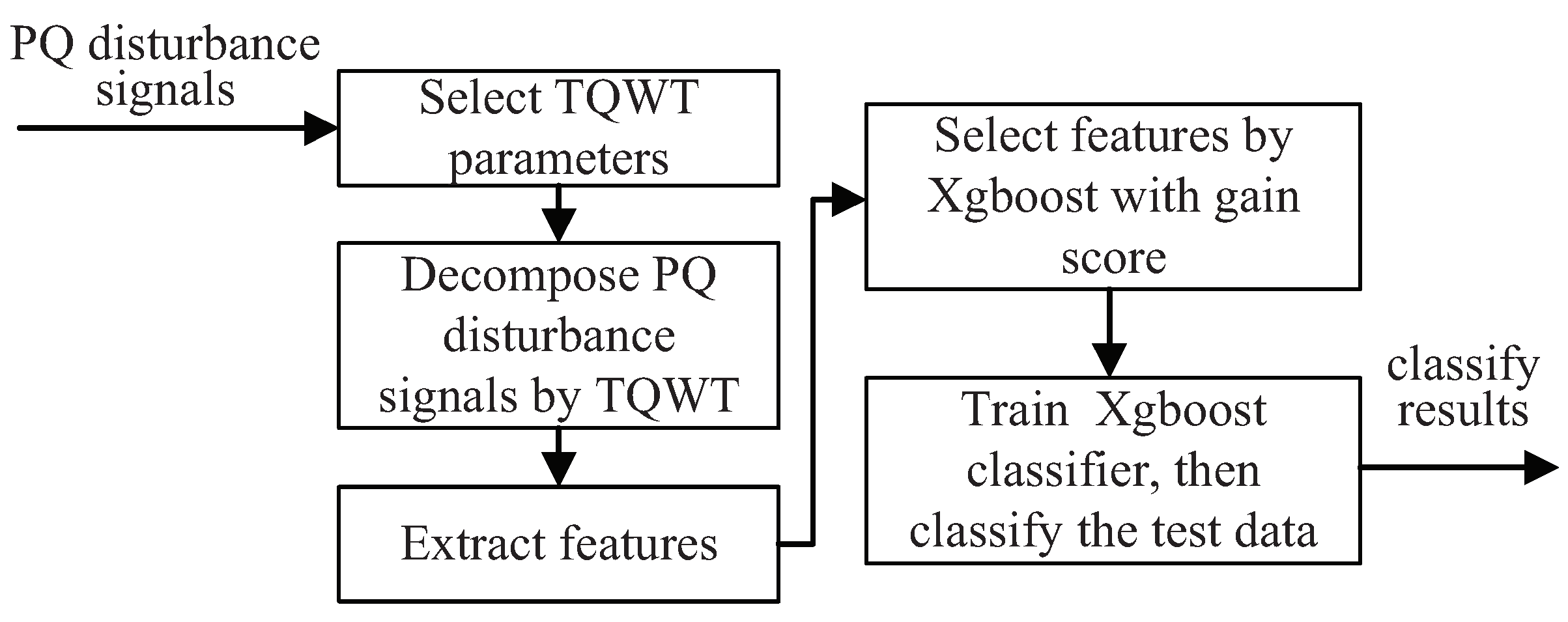
In this work, a novel technique is proposed to extract the features of sub-band signals, decomposed from PQ disturbances, by using tuning parameter optimization TQWT, and to select features and classify multiple PQ disturbances using the XGBoost algorithm. The flowchart of the proposed method is given in Figure 1.
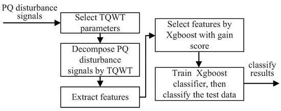
Figure 1.
The proposed method framework.
2.1. Tunable-Q Wavelet Transform
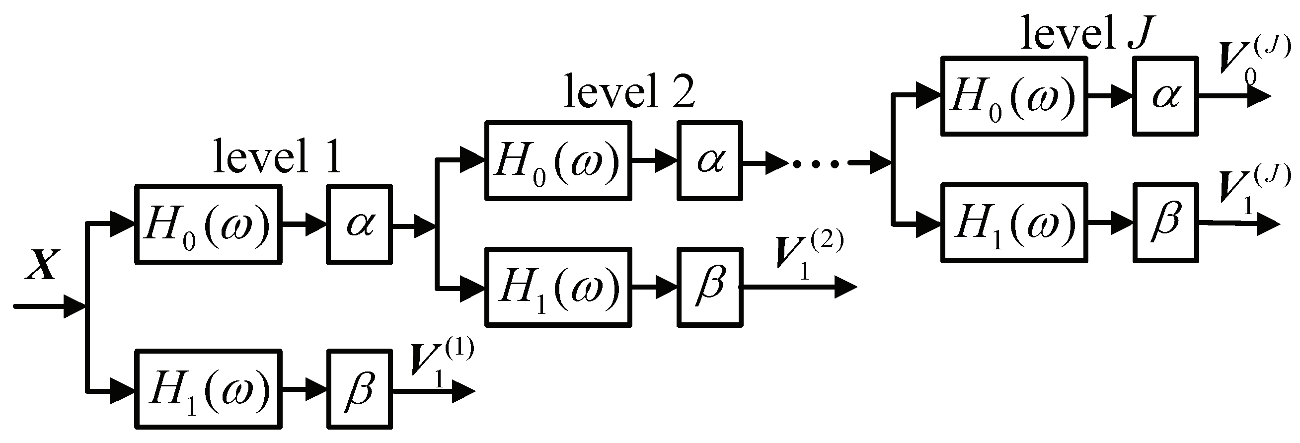
As an improvement of DWT, TQWT is suitable to analyze the oscillatory behavior of the input signal by using tunable parameters [15], i.e., Q-factor, redundancy (r) rate and the number of decomposition level (J). In TQWT, J-level sub-band signals (, ) are generated by the J decomposition of input signal , where and are the low-pass sub-band signal (LPS) and high-pass sub-band signal (HPS), respectively. At each decomposition level, two-channel filter banks are iteratively used at LPS, as shown Figure 2.

Figure 2.
The cascaded filter banks of TQWT.
In J-level decomposition, the frequency response of the low-pass filter and that of the high-pass filter are given by
and
respectively, where and are defined in terms of which is the Daubechies frequency response [15] with two vanishing moments, expressed as
where and are the low-pass and high-pass scaling, given by
After decomposition in the J levels, is decomposed into J HPSs, permuted in terms of frequency decreasing as (), and one LPS, denoted as , as shown in Figure 2.
2.2. Parameter Selection of TQWT
Tunable parameters need to be preset in TQWT implementation. Generally, the Q-factor controls the oscillation within the involved wavelet. The larger Q is suitable for the oscillatory signals while the smaller Q is suitable for smooth signals. The parameter r governs the overlapping of the frequency responses. The higher r helps in the better time localization of the wavelets. The scale J denotes the level of TQWT decomposition, determining the number of sub-band signals. To effectively decompose PQ disturbance signals for feature extraction [15], three parameters need to be accurately selected.
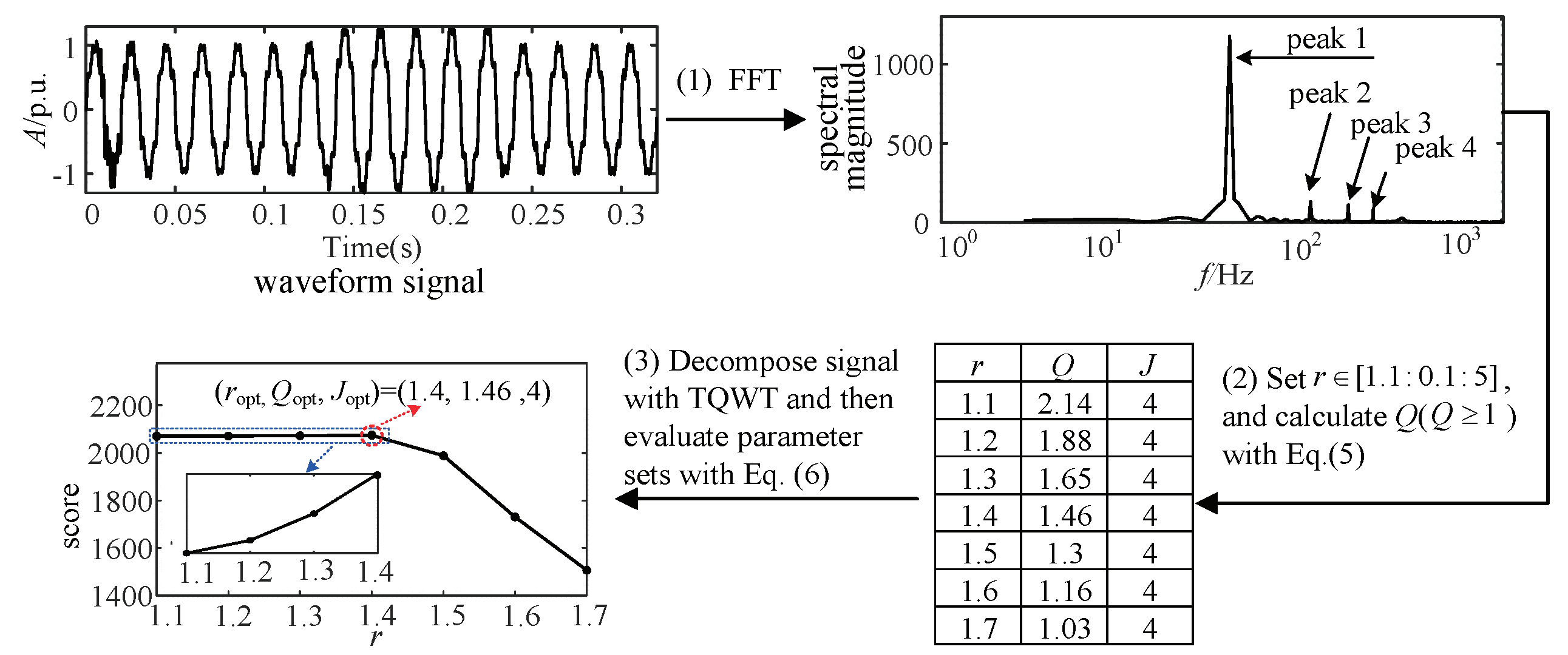
The scale J is firstly determined as the number of dominant-frequency components of the input signal , and the value of J needs to be lower than its maximum, i.e., , where N is the length of . Usually, a smaller J causes the aliasing of different components; a larger J causes false components and brings high computational cost. The ideal decomposition is to precisely divide the input signal into a series of narrowband components according to the dominant frequencies. Therefore, it is reasonable to determine J as the number of dominant frequency components. In our work, the number of dominant frequencies is counted as the number of the spectrum peaks of the input signal.
After J is determined, Q and r are selected to ensure that the fundamental component is exactly extracted from , since the fundamental component with 50 Hz or 60 Hz frequency is an essential one for different PQ disturbance signals. Compared with harmonic and other oscillation components, the fundamental component has lower frequency, and thus it is reasonable to use a low-pass filter to separate the fundamental component from the others. At J-level decomposition, the center frequency of the low-pass filter can be expressed as [16], where is the sampling frequency. To obtain the fundamental component in the low-frequency sub-band signal , after setting and using Equation (4), the relation between Q and r is written as
where is the fundamental frequency.
However, there is more than one solution when two sets of unknown Q to r with only one equation are involved. When (Q, r) are not properly selected, the desired decomposition cannot be obtained. For example, three different sets of (Q, r) and fixed J are used to decompose the PQ disturbance signal shown in Figure 3a, where its spectral magnitude in the second row of Figure 3a shows that the signal is composed of multi-frequency components. After the PQ disturbance signal is decomposed with different (Q, r), the extracted fundamental components () and corresponding spectral magnitudes are shown in Figure 3b–d. Figure 3b shows that is mixed with other components, having multiple peaks in its spectrum. Figure 3c shows that the value of the spectral magnitude of is largely less than that of the real one, indicating that part of is decomposed into other sub-bands. Only when (Q, r) are appropriately selected is the fundamental component correctly decomposed from the input signal, as shown in Figure 3d. In our work, to determine the proper Q and r, based on the spectral information from , an evaluation function is defined as
where is the spectral magnitude of and is the mean value of . The aliasing of different components is constrained by the first term in Equation (6), and the magnitude decreasing of fundamental component is restricted by the second term in Equation (6). Finally, appropriate (Q, r) with maximum are selected from a whole set of parameter candidates for the PQ disturbance signal with multi-frequency components. Considering the practicality and efficiency of TQWT implementation, the selected (Q, r) for the PQ signal with multiple components are used for other PQ disturbance signals. In summary, the algorithm of the parameter selection of TQWT is summarized in Algorithm 1.
| Algorithm 1 Algorithm for (J, Q, r) selection in TQWT. |
Input: Given input signal , and a set of candidates , where is the step size of r Iteration: Set , where is the number of main peaks in the spectral magnitude of . for do Compute Q via (5); Use to decompose by using TQWT; Compute via Equation (6); end for Determine appropriate (J,Q,r) with the maximum of . |
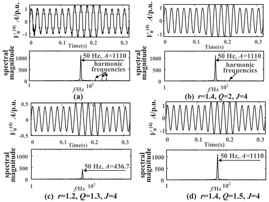
Figure 3.
Analysis of fundamental frequency components’ extraction. (a) three different sets of (Q, r) and fixed J are used to decompose the PQ disturbance signal; (b) is mixed with other components; (c) the value of the spectral magnitude of is largely less; (d) the fundamental component correctly decomposed from the input signal.
2.3. Sub-Band Selection and Feature Extraction
To reflect more helpful information hidden in decomposed sub-bands, feature extraction is performed for the design of a well-performing classifier. In addition, to reduce the influence of noise on the feature extraction, sub-band signals are determined on a selective basis. Considering that noise is commonly located in the high-frequency band and corresponds to the highest frequency sub-band in TQWT decomposition, is excluded from the experiments, while the other decomposed sub-band signals, i.e., , are used to perform feature extraction.
Features are the statistical measures in time and frequency domains for the selected sub-bands of PQ disturbance signals. Supposing that the length of is N and the length of per cycle is L, 16 features, i.e., - , are mathematically calculated for each as follows.
- and : the maximum and standard deviation of .where is the mean of .
- and : the operation related to the mean and median of the signal. .where .
- : the absolute error between the maximum and minimum of .
- : the energy ratio between and all selected sub-bands.
- : the crest factor of .
- and : the kurtosis and maximum of the spectral magnitude of ,where , is to operate fast Fourier transform, and .
- and : the maximum values and minimum values of the periodic root mean square (RMS) sequence .where for cycle.
- and : the maximum and minimum values of the periodic energy sequence ,where for cycle.
- : the maximum value of , where represents the number of zero crossings within cycle of .
- and : the standard deviation of instantaneous amplitude () and instantaneous frequency () sequence of the Hilbert–Huang transform of ,where and .
2.4. XGBoost-Based Feature Selection and Classification
After the feature vectors are constructed, they are used to build an XGBoost model to implement the classification of multiple PQ disturbances in this work, because XGBoost has the ability to deal with high-dimensional features and achieve high classification accuracy with high efficiency. In most cases, there would be much redundancy among a large number of extracted initial features, which might have negative impacts on the process of classification. Hence, it represents a comprehensive feature selection scheme for successful classification. This selection scheme contributes significantly to the simplified modeling of classification. In addition, XGBoost, as a boosting tree-based classification method, has a mechanism to give an importance score for each feature. Thus, the XGBoost algorithm integrates feature selection and a learning–training process to improve the efficiency of classification.
In contrast to classical gradient boosting decision trees (GBDT), XGBoost performs a second-order Taylor expansion of the loss function, and combines first-order with second-order derivatives to make the model convergent more quickly. Denoting the input as with n examples and the target as , the second-order Taylor series of the loss function at the t-th iteration can be expressed as
where is the error function of the predicted and the target , the variables and are the first derivative and second derivative of the error function, respectively; is leaf node score of the t-th tree, c is constant, and is a regularization term, given by
where T is the total number of leaf nodes and is the score of each leaf node; and are penalty coefficients; measures the complexity of the training model to avoid over-fitting. Together, these advantages make XGBoost potentially more efficient to achieve a better classification accuracy than the classical GBDT. A detailed description of the XGBoost algorithm is given in [11].
Apart from its capability in modeling non-linear classification, XGBoost is also able to rank the feature importance measured by ’weight’ and ’gain’, etc. ’Weight’ is the number of times that a feature is used to split the data across all boosted trees; ’gain’ is the average gain across all splits in which the feature is used [17]. When training XGBoost in this paper, ’gain’ is used to determine the split node, expressed as
where and represent the samples of the left and right nodes after the split. . The higher the gain is, the more important the corresponding feature is. Thus, the importance score of each feature can be obtained for ranking.
The optimum feature set can thus be selected owing to the classification accuracy of the XGBoost algorithm. All extracted features are first ranked according to its value of ’gain’. Then, the XGBoost model is trained with these ranked features, and the classification accuracy recorded. By iteratively removing the last feature in the ranked feature sets, the above steps are repeated until only one feature is left. As the removal of less effective features contributes significantly to the improvement of the learning model, the optimum feature set is selected on an accuracy basis. The program flow chart of XGBoost for feature selection is shown in Figure 4.
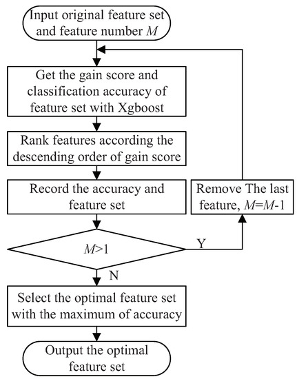
Figure 4.
The program flow chart of feature selection in the XGBoost algorithm.
3. Experiments and Results
To evaluate the proposed method, 26 categories of synthetic single and complex PQ disturbances were tested for classification. Basic 7 single PQ disturbances were generated based on the mathematical models presented in Ref. [18] labeled as: sag (C1), swell (C2), oscillation transient (C3), impulsive transient (C4), harmonic (C5), interruption (C6) and flicker (C7), respectively. The other 19 complex PQ disturbances listed in Table 1 are compounded by combining different single PQ disturbance as Ref. [18] does.

Table 1.
Classification accuracy of the proposed method at different noisy levels for synthetic data.
To prevent loss of information, the sampling frequency is set as 6.4 KHz for generating the 0.3 s waveform signal. A total of 20,800 signals with 800 signals of each class were randomly generated according to the IEEE recommended standard [19], with 13,000 signals as training data, 3900 signals as validation data, and 3900 signals as test data. Moreover, to test the robustness of the method, these synthetic signals are run under four different noise levels, and the signal-to-noise ratio (SNR) is set to be 50 dB, 40 dB, 30 dB and 20 dB. All experiments are implemented on a personal computer with an AMD processor of 3.6 GHz and 8 GB RAM. The classification accuracy of a class j is computed as
where is the number of correctly recognized signals of the class j, and is the total number of test signals of that class.
3.1. The Results of PQD Signal Decomposition
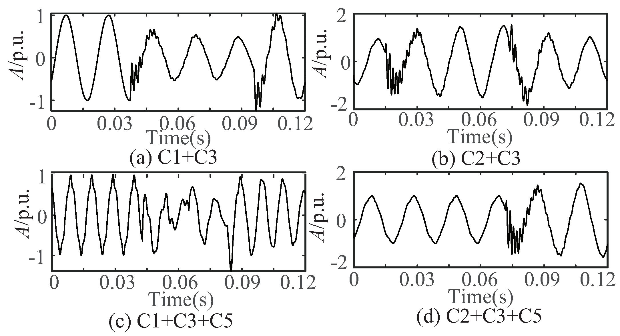
To efficiently implement TQWT for decomposing PQD signals, three parameters (r,Q,J) were selected, as described in Section 2.2. A complex signal with multiple components, labeled as C2+C3+C5, was empirically utilized to determine the values of the three parameters. The determination procedure is shown in Figure 5. According to the number of dominant components in the spectral magnitude of C1+C3+C5 signal, the J was first set to , and then with maximum in (6) are determined. The obtained are also used for other PQ disturbance signal decomposition.
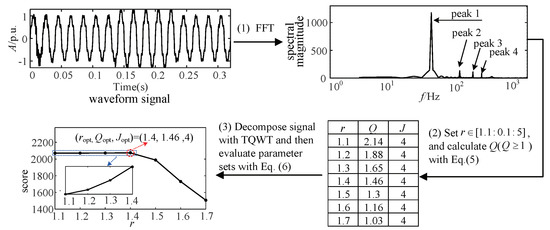
Figure 5.
The procedure of parameter selection for TQWT.
Figure 6a–c present the TQWT decomposition results of three types of PQ disturbances, i.e., sag (C1), harmonic+flicker (C5+C7) and swell+oscillation transient+harmonic (C2+C3+C5), respectively. It can be seen that the fundamental frequency component is better extracted into the sub-band s, the oscillation component is distributed in , and the harmonics components are mainly distributed in and . In addition, the noise component is separated into sub-band plotted in red line. In summary, Figure 6 illustrates that multiple frequency components of different PQ disturbance signals can be clearly separated by TQWT decomposition with proper values of .
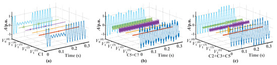
Figure 6.
The decomposition results of TQWT with parameter selection for three PQ disturbance signals: (a) sag (C1); (b) harmonic+flicker (C5+C7); and (c) swell+oscillation transient+harmonic (C2+C3+C5).
3.2. The Results of Feature Selection
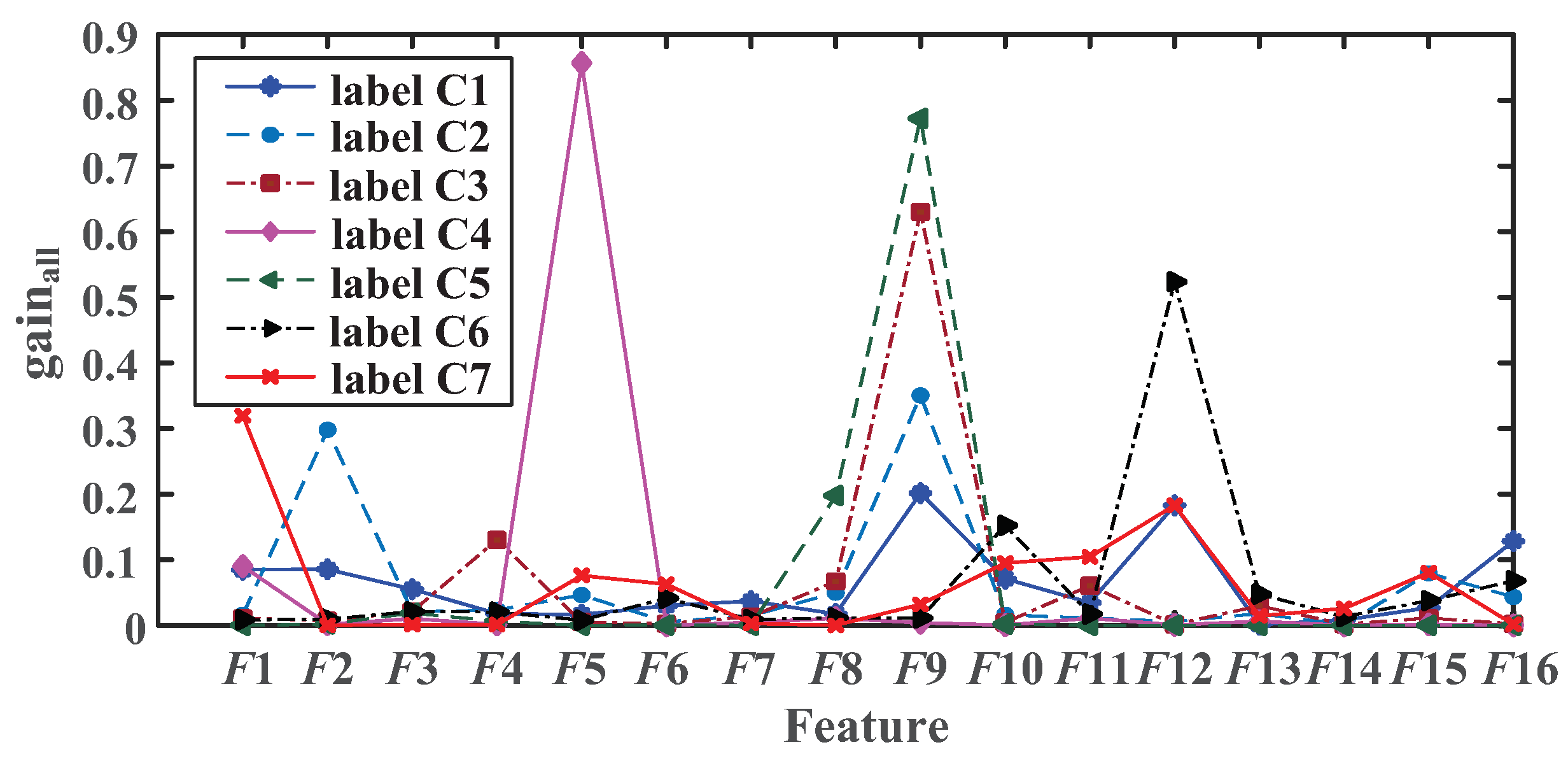
The four decomposed sub-bands, , are used to extract features, since noise in a high-frequency component mainly exists in the sub-band . Actually, among the 64 extracted features, with 16 features for each of the 4 sub-bands concerned, some turn out to be irrelevant to the classification of PQ disturbances. For example, for seven basic PQ disturbance labels, we measure the overall importance of the 16 features and plot it in Figure 7, where is calculated as the sum of the corresponding feature importance in four sub-bands, which, in turn, is evaluated as in Equation (25). Figure 7 illustrates that the effective features for different labels differ from each other, indicating the necessity of feature selection.
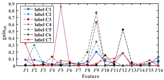
Figure 7.
Feature importance analysis.
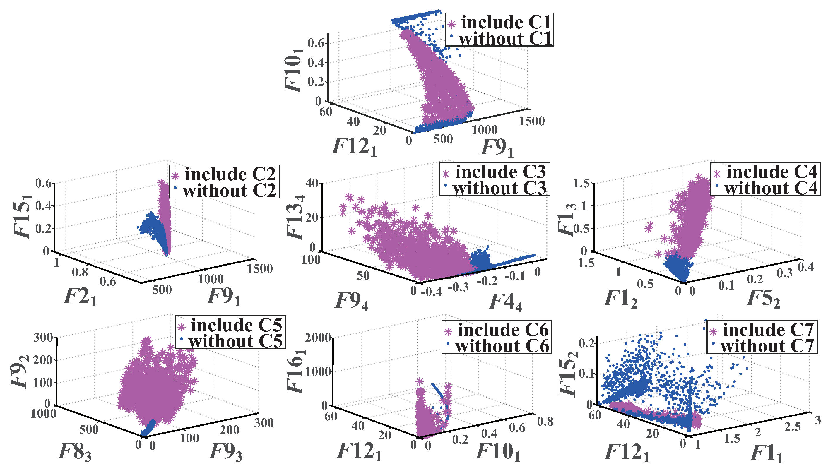
After XGBoost-based feature selection, the optimum feature sets are obtained for seven basic PQ disturbance labels, as shown in Table 2. The dimensions of optimum feature sets are at least reduced from 64 to 18. Furthermore, to demonstrate the validity of XGBoost-based feature selection, Figure 8 shows the scatter plots constructed by the top three optimum features of each label in Table 2, where each label can be well distinguished.
Table 2.
Feature importance analysis.
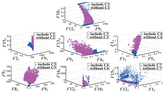
Figure 8.
Scatterplot of the top three optimum features for each label in Table 2.
3.3. Classification Experiment
The proposed classification method was evaluated by using synthetic signals and field data measured in a station located in Nanjing, China. The classification model is trained with the selected features from the synthetic signals, since there are only a few field data available. After that, the trained model was used to classify the synthetic test data and field data.
For synthetic test data, the accuracy of classification is taken into consideration to evaluate the performance of the model. First, under different SNRs, the proposed method is used to classify 26 types of PQ disturbances. The accuracy results for each class and average accuracy for different SNRs are shown in Table 1. It can be seen that when SNR = 20 dB, the average classification accuracy is 97.63%; when SNR = 50 dB, the average classification accuracy reaches 99.27%. Table 1 illustrates that the proposed method has strong robustness to noise and high recognition accuracy.
Considering that VMD and DWT, like TQWT, are also commonly used as time-frequency decomposition methods, and random forest (RF) and DT are widely-used learning models of classification, they are combined to construct new classification models in comparison with the proposed model. The average accuracy results of different combinations are shown in Table 3. In DWT, ’db8’ is selected as a mother wavelet, and six-level decomposition is performed. In VMD, two key parameters are set, i.e., the number of extracted modes as and the balancing parameter as . Table 4 shows that the proposed method achieves the highest average accuracy among various combinations, especially when SNR = 20 dB.
Table 3.
Performance comparison of proposed method with other combination methods.
Table 4.
Performance comparison of proposed method with other existing methods.
The proposed method is then compared with five existing methods, including DWT + probabilistic neural network (PNN) [2], TQWT + Multiclass SVM [15], cross-wavelet transform (CWT) + SVM [20], image enhancement technique (IMT) + RF [21] and TQWT + RF [22]. Because of the similarity in the data and performance evaluation method, we directly quote the accuracy results of these methods from corresponding publications and present the results in Table 4. From Table 4, it can be seen that when SNR = 20 dB, the proposed method shows the best classification accuracy and identifies more types of PQ disturbances, although the accuracy of the proposed method is slightly lower than CWT + SVM and IMT + RF, when the SNR ≥ 40 dB. Meanwhile, TQWT exhibits better classification accuracy after the parameters have been fine-tuned, demonstrating that improved TQWT extracts more effective features than conventional TQWT.
Finally, to evaluate the practicability of the proposed method, 22 groups of field PQ disturbances are used in this experiment. In contrast to multiple types of PQ disturbance in synthetic data, only two types of single PQ disturbance and five types of complex PQ disturbances were captured in fault recorder. Some waveforms are shown in Figure 9, where the sampling frequency is 12.8 KHz, and the ground-truth class for each waveform signal is judged by personal experience. After the classifier is trained using synthetic data with the same specifications, it is applied in these measured PQ disturbances. Due to the small number of field data, using accuracy as an indicator of classification performance lacks statistical significance in this case. Thus, the numbers of correct and incorrect classifications are instead provided in Table 5. As is shown, the real PQD signals can be relatively better classified.

Figure 9.
The field PQ disturbance signals captured in fault recorder.
Table 5.
Classification results of measured PQD signals.
4. Conclusions
This paper presents a novel method of integrating improved TQWT with XGBoost to classify multiple PQ disturbances efficiently. The spectral information of multiple PQ disturbances is first used to fine-tune the parameters of TQWT, conducive to extracting the effective features even in the noisy case. Furthermore, then, the feature selection and the PQ disturbance classification are implemented in XGBoost, which simplifies the process and ensures a higher classification accuracy. The major finding from the result can be summarized as follows:
- The decomposition results of the improved TQWT are better than those of TQWT, VMD and DWT. Meanwhile, the proposed screening method for sub-bands also improves the noise-resistance performance;
- It performs well with 97.63% accuracy in the 20 dB noisy case, and the classification accuracy reached above 99% with low noise cases;
- Compared with the results from recently published related works, the accuracy of the proposed method outperforms PNN, SVM, and other methods;
- The classification accuracy of the proposed method is slightly lower than that of IWT in the 30 dB and 50 dB noise cases, while IWT extracts more valuable features at the expense of algorithmic complexity.
In future work, we expect that the proposed method can be used to classify multiple PQ disturbances in real-time and be applied in a real power station, e.g., renewable energy sources.
Author Contributions
Conceptualization, L.Y. and L.G.; methodology, L.Y., L.G. and X.Y.; validation, W.Z. and X.Y.; investigation, L.Y.; data curation, L.G.; writing—original draft preparation, X.Y.; writing—review and editing, W.Z.; visualization, L.Y. All authors have read and agreed to the published version of the manuscript.
Funding
This research received no external funding.
Institutional Review Board Statement
Not applicable.
Informed Consent Statement
Not applicable.
Data Availability Statement
Not applicable.
Conflicts of Interest
The authors declare no conflict of interest.
Nomenclature
| PQ | power quality |
| TQWT | tunable-Q wavelet transform |
| STFT | short-time Fourier transform |
| DWT | discrete wavelet transform |
| ST | S-transform |
| EMD | empirical mode decomposition |
| VMD | variational mode decomposition |
| SVM | support vector machine |
| DT | decision trees |
| ANN | artificial neural network |
| CDT | classification decision tree |
| RF | random forests |
| XGBoost | extreme gradient boosting |
| GBDT | gradient boosting decision trees |
| PNN | probabilistic neural network |
| CWT | cross-wavelet transform |
| IMT | image enhancement technique |
References
- Heydt, G.T.; Fjeld, P.S.; Liu, C.C.; Pierce, D.; Tu, L.; Hensley, G. Applications of the windowed FFT to electric power quality assessment. IEEE Trans. Power Deliv. 1999, 14, 1411–1416. [Google Scholar] [CrossRef]
- Khokhar, S.; Mohd Zin, A.A.; Memon, A.P.; Mokhtar, A.S. A new optimal feature selection algorithm for classification of power quality disturbances using discrete wavelet transform and probabilistic neural network. Measurement 2017, 95, 246–259. [Google Scholar] [CrossRef]
- Singh, U.; Singh, S.N. Optimal Feature Selection via NSGA-II for Power Quality Disturbances Classification. IEEE Trans. Ind. Informatics 2018, 14, 2994–3002. [Google Scholar] [CrossRef]
- Zhang, S.; Li, P.; Zhang, L.; Li, H.; Jiang, W.; Hu, Y. Modified S transform and ELM algorithms and their applications in power quality analysis. Neurocomputing 2016, 185, 231–241. [Google Scholar] [CrossRef]
- Sahani, M.; Dash, P.K. Automatic Power Quality Events Recognition Based on Hilbert Huang Transform and Weighted Bidirectional Extreme Learning Machine. IEEE Trans. Ind. Inform. 2018, 14, 3849–3858. [Google Scholar] [CrossRef]
- Sahani, M.; Dash, P.K.; Samal, D. A real-time power quality events recognition using variational mode decomposition and online-sequential extreme learning machine. Measurement 2020, 157, 07597. [Google Scholar] [CrossRef]
- Achlerkar, P.D.; Samantaray, S.R.; Manikandan, M.S. Variational Mode Decomposition and Decision Tree Based Detection and Classification of Power Quality Disturbances in Grid-Connected Distributed Generation System. IEEE Trans. Smart Grid 2018, 9, 3122–3132. [Google Scholar] [CrossRef]
- Guan, C.; Zhou, L.; Lu, W. Recognition of Multiple Power Quality Disturbances Using Multi-Label RBF Neural Networks. Trans. China Electrotech. Soc. 2011, 26, 198–204. [Google Scholar]
- Yi, L.; Li, K.; Li, Y.; Cai, D.; Chen, Z.; Meng, Q. Three-Layer Bayesian Network for Classification of Complex Power Quality Disturbances. IEEE Trans. Ind. Inform. 2018, 14, 3997–4006. [Google Scholar]
- Lin, W.M.; Wu, C.H.; Lin, C.H.; Cheng, F.S. Detection and Classification of Multiple Power-Quality Disturbances With Wavelet Multiclass SVM. IEEE Trans. Power Deliv. 2008, 23, 2575–2582. [Google Scholar] [CrossRef]
- Chen, T.; Guestrin, C. XGBoost: A scalable tree boosting system. In Proceedings of the 22nd ACM SIGKDD International Conference on Knowledge Discovery and Data Mining, KDD 2016, San Francisco, CA, USA, 13–17 August 2016; pp. 785–794. [Google Scholar]
- Guo, J.; Yang, L.; Bie, R.; Yu, J.; Gao, Y.; Shen, Y.; Kos, A. An XGBoost-based physical fitness evaluation model using advanced feature selection and Bayesian hyper-parameter optimization for wearable running monitoring. Comput. Netw. 2019, 151, 166–180. [Google Scholar] [CrossRef]
- Liu, Y.; Yi, L.; Cheng, D. Application of XGBoost in Identification of Power Quality Disturbance Source of Steady-state Disturbance Events. In Proceedings of the 2019 IEEE 9th International Conference on Electronics Information and Emergency Communication (ICEIEC), Beijing, China, 12–14 July 2019. [Google Scholar]
- Amirou, A.; Amirou, Y.; Ould-Abdeslam, D. S-Transform with a Compact Support Kernel and Classification Models Based Power Quality Recognition. J. Electr. Eng. Technol. 2022, 1, 1–10. [Google Scholar] [CrossRef]
- Thirumala, K.; Prasad, M.S.; Jain, T.; Umarikar, A.C. Tunable-Q Wavelet Transform and Dual Multiclass SVM for Online Automatic Detection of Power Quality Disturbances. IEEE Trans. Smart Grid 2018, 9, 3018–3028. [Google Scholar] [CrossRef]
- Selesnick, I.W. Wavelet transform with tunable Q-factor. IEEE Trans. Signal Process. 2011, 59, 3560–3575. [Google Scholar] [CrossRef]
- Shi, X.; Wong, Y.D.; Li, M.Z.; Palanisamy, C.; Chai, C. A feature learning approach based on XGBoost for driving assessment and risk prediction. Accid. Anal. Prev. 2019, 129, 170–179. [Google Scholar] [CrossRef] [PubMed]
- Wang, S.; Chen, H. A novel deep learning method for the classification of power quality disturbances using deep convolutional neural network. Appl. Energy 2019, 235, 1126–1140. [Google Scholar] [CrossRef]
- IEEE Std 1159.3-2003; IEEE Recommended Practice for the Transfer of Power Quality Data. IEEE std: New York, NY, USA, 2004; pp. 1–138.
- Dalai, S.; Dey, D.; Chatterjee, B.; Chakravorti, S.; Bhattacharya, K. Cross-Spectrum Analysis-Based Scheme for Multiple Power Quality Disturbance Sensing Device. IEEE Sens. J. 2015, 15, 3989–3997. [Google Scholar] [CrossRef]
- Lin, L.; Wang, D.; Zhao, S.; Chen, L.; Huang, N. Power Quality Disturbance Feature Selection and Pattern Recognition Based on Image Enhancement Techniques. IEEE Access 2019, 7, 67889–67904. [Google Scholar] [CrossRef]
- Yang, X.; Guo, L.; Xiao, X.; Zhang, J. Classification of Multiple Power Quality Disturbances Based on TQWT and Random Forest Feature Selection Algorithm. Power Syst. Technol. (Chin.) 2020, 44, 3014–3020. [Google Scholar]


Publisher’s Note: MDPI stays neutral with regard to jurisdictional claims in published maps and institutional affiliations. |
© 2022 by the authors. Licensee MDPI, Basel, Switzerland. This article is an open access article distributed under the terms and conditions of the Creative Commons Attribution (CC BY) license (https://creativecommons.org/licenses/by/4.0/).