The Impact of Oil Price Fluctuations on Consumption, Output, and Investment in China’s Industrial Sectors

Abstract

This paper aims to simulate and evaluate the impacts of increases and decreases in oil price on industrial sectors in China. We develop an oil-economy computable general equilibrium (OE-CGE) model with crude oil as an important factor in production. The transmission mechanism of crude oil price swings to various industrial sectors is described in the model. We calibrate parameters in the model parameters using input-output data. In addition, we simulate the rise and fall of oil prices in the model and assess the impact of crude oil prices on various industrial sectors. The results show that crude oil price changes have the greatest impact on the output and consumption of crude oil and gas extraction products sector, crude oil refined coke products, and processed nuclear fuel products sector. The investment of public utilities sector is the most sensitive to changes in crude oil price. When the price of crude oil changes, its investment drops significantly. Crude oil price stability is extremely important for investment and output stability in all sectors.

1. Introduction

Crude oil price has fluctuated dramatically over the 20th century. Between 1980 and 1997, crude oil price continued to fall and remained low. Between 1997 and 2008, oil price continued to rise during the two financial crises. From 2008 to the present, oil price has fluctuated frequently and there has been massive oil price increases. Large fluctuations in oil prices can affect not only the production costs of related industries but also the investment decisions of capital markets. If risks are not prevented in time, the economies of countries around the world, especially crude oil-importing countries, will be seriously affected.

China is a major importer of crude oil, and crude oil price fluctuations have a huge impact on the Chinese economy. China’s crude oil production has been increasing year by year, but it is still difficult to meet domestic economic activities. Due to the influence of crude oil reserves and exploration and production technologies, the increase in crude oil demand is greater than the increase in crude oil production, and the domestic supply is insufficient. China’s energy market is highly dependent on the international energy market, and rising crude oil price will increase production and operating costs in various domestic industrial sectors and harm production and operating activities, while falling crude oil price will make the market unbalanced. Therefore, the impact of crude oil price fluctuations on various industrial sectors should be taken seriously. Clarifying how crude oil price fluctuations affect various industries can stabilize the economy to a certain extent and help prevent the risk of oil price fluctuations. It can also provide solutions for industries to avoid risks and reduce economic losses in the event of crude oil price fluctuations.

This paper focuses on the impact of crude oil price fluctuations on consumption, investment, and output in China’s industrial sectors. The possible marginal contributions of this paper are as follows: A crude oil-economy computable general equilibrium model is constructed based on the standard computable general equilibrium model with crude oil as the basic factor of production input. Unlike other literature studies that have examined the impact of crude oil price fluctuations on the overall macroeconomy, this paper uses the CGE model to refine the impact of crude oil price changes on the economy to individual industry sectors, which can help each industry sector to reasonably hedge risks associated with crude oil price fluctuations.

This study is structured as follows. In Section 2, we mainly review the relevant literature. Section 3 focuses on model construction by constructing a crude oil-economy computable general equilibrium (OE-CGE) model to build the foundation for conducting numerical simulations later on. The Section 4 mainly calibrates the parameters of Leontief, CES, and CET functions and the propensity to save before simulating the CGE model to provide accurate a priori data for the later numerical simulations. Section 5 derives the corresponding results from the numerical simulations. Section 6 contains conclusions, policy recommendations, and limitations.

2. Literature Review

In recent years, frequent occurrence of conflicts in Middle East, Russia-Ukraine, and other areas have made the crude oil market more volatile than ever. China relies on imported crude oil to sustain high-quality economic development, and the uncertainty in the international crude oil market has heightened the need to asses the impacts of oil price fluctuations on China’s economy. While studies have found that the fluctuations of crude oil market do not have a significant impact on economic growth in the short run [1], they have found that oil price fluctuations clearly impede economic growth in the long run [2]. Specifically, negative oil price fluctuations break the international trade balance and trigger inflation, which in turn threatens the quality development of the economy [3]. A positive oil price uncertainty shock, on the other hand, can lead to a decline in real economic activity, world crude oil production, and world crude oil prices in all countries [4], with the same adverse effects. Studies about the impact of oil price fluctuations on the economy are briefly reviewed as follows.

There are studies on the relationship between crude oil prices and macroeconomic variables. Liu et al. concluded that large increases in oil prices have a significant negative impact on economic growth and money supply and that economic growth responds more persistently than other economic variables [5]. Yildirim and Arifli [3] studied the impact of falling oil prices on the economy and found that falling oil prices worsen the trade balance, lower the real exchange rate, depreciate the currency, increase inflation, and force a recession. Kim et al. [6] had a different conclusion that the foreign exchange market is resistant to crude oil price fluctuations and that external shocks from crude oil price fluctuations can hardly affect the exchange rate market. Mohaddes and Pesaran found a stable negative correlation between oil prices and real dividends and that the crude oil market exhibited significant cyclical fluctuations between low and high oil prices [7]. Mallick et al. [8] noted that shocks from crude oil price volatility have a significant negative impact on private investment. Lorusso [9] found that crude oil price shocks have a non-negligible impact on the UK macroeconomic aggregates, mainly in terms of unemployment, inflation, etc. Guan et al. [1] argued that crude oil price fluctuations may harm economic growth as measured by GDP in resource producing economies in the long run. Jin et al. [10] argued that different levels of crude oil price fluctuations have different dampening effects on the consumer price index and similar effects on GDP. Scholars chose different macroeconomic variables in their studies, but concluded uniformly that significant effects of oil price shocks on the economy do exist.

There are studies on the asymmetric impact of oil price changes on the economy. Nasir et al. [11] reached a similar conclusion that there are significant differences and asymmetries in the response to oil fluctuations in economies with different economic structures. This finding was validated by subsequent studies. Charfeddine [12] found that there is asymmetry in the short-run oil price shocks to the economy, i.e., both real GDP and non-crude oil real GDP respond more to negative shocks than positive shocks. Nusair [13] argued that the impact of higher oil prices on output is more than that of a fall in oil prices, and this asymmetric impact varies by country. In contrast, Cheng et al. [14] reached an opposite conclusion and argued that positive uncertainty shocks of oil prices depress real GDP and investment, while negative uncertainty shocks to oil prices tend to boost the macroeconomy by increasing investment and real GDP.

A series of literature has analyzed factors affecting the economic impact of crude oil price changes. Khan et al. [15] identified the world economic expansion, mismatch of crude oil supply and demand mismatch, and dollar depreciation as the dominant factors of crude oil price fluctuations that shock the economy. Jia et al. [16] identified factor inputs as the main influencing factor for the economic impact effect of crude oil price fluctuations compared to consumer preferences factors. Lorusso and Pieroni [9], on the other hand, explained the impact of oil price fluctuations on the economy in terms of demand and supply shocks and found that specific demand shocks largely affect the growth of the economy, especially the fluctuations in GDP growth and unemployment rate.

In this paper, we follow a few studies that analyze the impact of crude oil price fluctuations on the economy across sectors. Thorbecke [17] stated that industries such as airlines, food, and industrial transport are harmed by higher oil prices, while industries such as oil and gas production and exploration are benefited, and the findings apply to most countries. Charfeddine and Barkat [12] argued that non-oil industries recover better than oil industries when crude oil prices generate negative shocks. Quintero [18] argued that production activities are slightly reduced in most sectors by aggregate demand shocks, and the sectors most directly affected are manufacturing, electricity, gas, and water. The findings serve as a validation for other related studies as well. These studies have engaged in a similar analysis of the macroeconomic impact of crude oil price changes but have not paid much attention to the impact on consumption, taxation, and output of specific industry sectors across the chain.

Scholars have studied oil price fluctuations and the national economy from different perspectives, but most of the studies are biased toward macroeconomic aggregates and lack a microscopic perspective. How the entire industry chain will be affected by oil price fluctuations and how each industry should change its production scale and investment strategy through oil price changes are the questions that we want to address in this paper. Therefore, we will study the impact of crude oil price changes on each industry sector by conducting numerical simulations, drawing on previous research by scholars. In this paper, we comprehensively simulate the effects of changes in crude oil price increases and decreases on consumption, investment, and output in each industrial sector and propose preventive policies to cope with future crude oil price shocks in order to stabilize the national economy.

3. Model Description

Following the standard computable general equilibrium model [19], we use crude oil as a factor of production in the model. In the OE-CGE model, capital, labor, and crude oil are combined into composite factors using the Cobb–Douglas technique. Then, the composite factor and the products of various industrial sectors as intermediate inputs are produced as intermediate products. In addition to domestic consumption, some intermediate products are used for export. Due to the substitutability between domestic and foreign products, domestic products and imported products are assumed to be synthesized for Armington goods by using a constant elasticity of substitution (CES) technique. Armington goods are final consumer goods for government consumption, household consumption, investment, and intermediate inputs. The structure of OE-CGE model can be descripted as Figure 1.

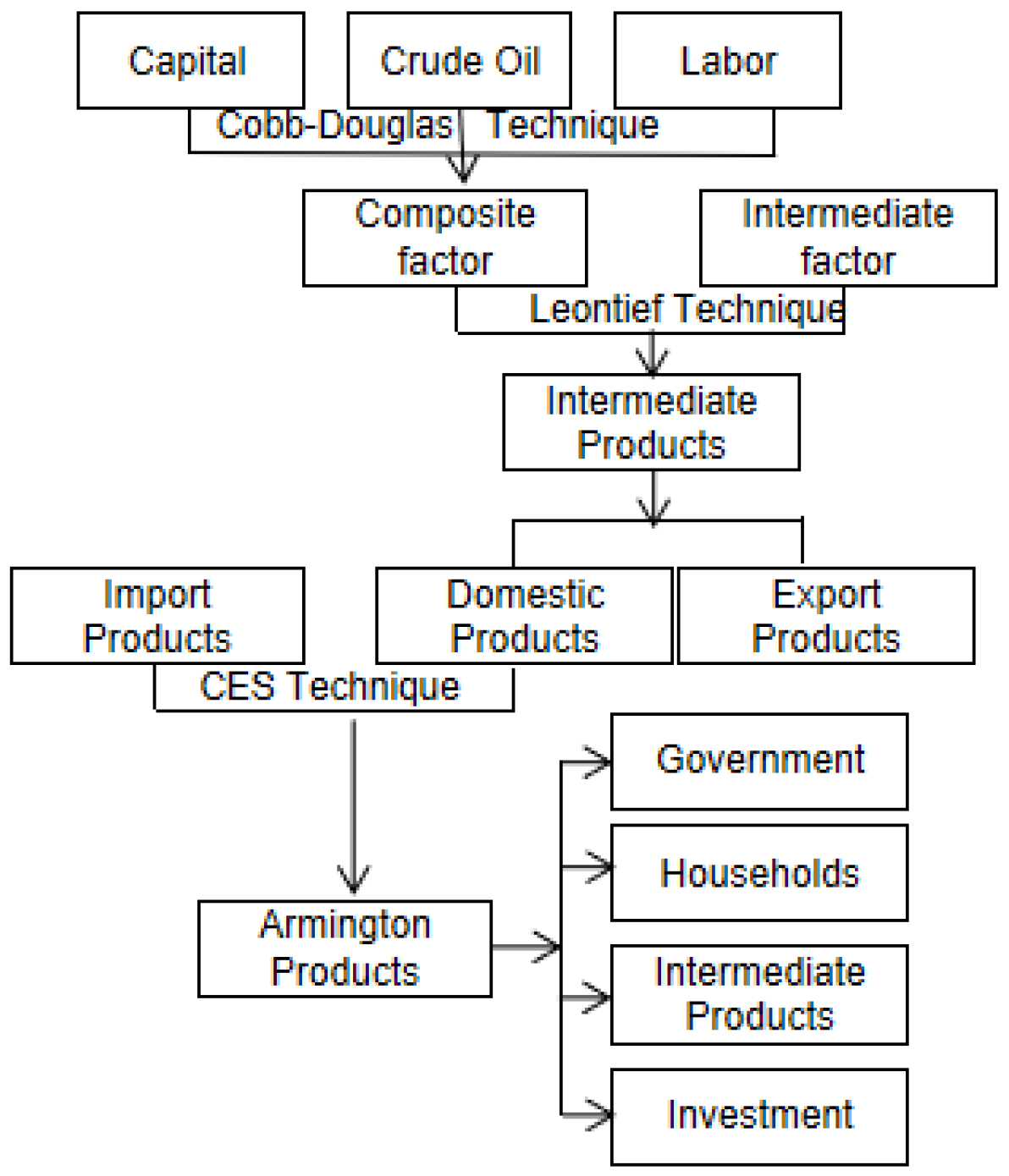
3.1. Production in Economy

In this paper, domestic production is divided into two stages. In the first stage, capital, labor, and crude oil are combined into a composite factor $Y_j$ for production using the Cobb–Douglas technique. The objection of profit maximum for firm j can be described as follows:

$$\underset{F_{c,j,}{F}_{l,j,}{F}_{oil,j}}{maximize}\hspace{1em}{\pi }_j^y=p_j^y{Y}_{{}_j}-p_c^f{F}_{c,j}-p_l^f{F}_{l,j}-p_{oil}^f{F}_{oil,j}$$

(1)

$$s.t.Y_j=b_j{F}_{c,j}^{{\beta }_{c,j}}{F}_{l,j}^{{\beta }_{l,j}}{F}_{\mathrm{oil},j}^{{\beta }_{oil,j}},\forall j$$

(2)

where ${\pi }_j^y$ denotes the profit of producing the composite factor; $Y_j$ denotes the quantity of the composite factor used in the second stage; $p_j^y$ denotes the price of the composite factor j; $F_{c,j}$, $F_{l,j}$, and $F_{oil,j}$ refer the quantity of capital, labor, and crude oil, respectively, invested in the first stage of production; $p_c^f$, $p_l^f$, and $p_{oil}^f$ denote the price of capital, labor, and crude oil, respectively; ${\beta }_{.,j}$ denotes the input share coefficient of various factors in the composite factor of production; $b_j$ denotes the scale coefficient of the composite factor production function.

In the second stage, the composite factor and the intermediate products are combined to produce total domestic output using Leontief technique. The objection of profit maximization for firm j can be written in the following form:

$$\underset{Z_{\mathrm{j}},Y_j,X_{i,j}}{maximinze}\hspace{1em}{\pi }_j^z=p_j^z{Z}_j-(p_j^y{Y}_j+\sum _i{p}_i^q{X}_{i,j})$$

(3)

$$s.t.Z_{\mathrm{j}}=min(\frac{X_{i,j}}{a{x}_{i,j}},\frac{Y_j}{a{y}_j})$$

(4)

where ${\pi }_j^z$ denotes the profit of the first stage firm producing the composite factor; $X_{i,j}$ denotes the quantity of the intermediate input product i used by firm j; $p_j^z$ denotes the price of the domestic output product j; $p_i^q$ denotes the price of the composite product i; $a{x}_{i,j}$ and $a{y}_j$ denotes the quantity of i intermediate inputs and j composite factor to produce a unit of product j. The production behavior of an enterprise can be expressed as follows.

$$Y_j=b_j\prod _h{F}_{h,j}^{{\beta }_{h,j}}{F}_{oil,j}^{{\beta }_{oil,j}},\forall j$$

(5)

$$F_{{}_{c,j}}=\frac{{\beta }_{c,j}{p}_j^y}{p_c^f}{Y}_j,\forall j$$

(6)

$$F_{{}_{l,j}}=\frac{{\beta }_{l,j}{p}_j^y}{p_l^f}{Y}_j,\forall j$$

(7)

$$F_{{}_{oil,j}}=\frac{{\beta }_{oil,j}{p}_j^y}{p_{oil}^f}{Y}_j,\forall h,j$$

(8)

$$X_{i,j}=a{x}_{i,j}{Z}_j,\forall i,j$$

(9)

$$Y_j=a{y}_j{Z}_j,\forall j$$

(10)

$$p_j^z=a{y}_j{p}_j^y+\sum _{i}a{x}_{i,j}{p}_i^q,\forall j$$

(11)

3.2. Government Description

We assume that government does not participate in production. The government should maintain a balanced budget. Government revenue comes from taxes on households or companies and tariffs on imported products. All the revenue is used for government consumption and transfers to households or businesses. The direct tax rate on households is ${\tau }^d$, and the tax amount is $T^d$. The indirect tax on firms is assumed to be ${\tau }_j^z$, and the tax amount is $T_j^z$. The tariff rate imposed on imported goods is ${\tau }_i^m$. The government’s savings is $S^g$, and the consumption of government is $X_i^g$. The tax revenue and consumption can be expressed as follows:

$$T^d={\tau }_d^z(p_c^f{F}_c+p_l^f{F}_l)$$

(12)

$$T_j^z={\tau }_j^z{p}_j^z{Z}_j,\forall j$$

(13)

$$T_i^m={\tau }_i^m{p}_i^m{M}_i,\forall i$$

(14)

$$X_i^g=\frac{{\mu }_i}{p_i^q}(T_j^z+T_i^m-S^g),\forall i,j$$

(15)

$$S^g=s{s}^g(T^d+\sum _j{T}_j^z+\sum _j{T}_j^m)$$

(16)

where $T_j^z$ is the indirect tax levied on the production of product j; $T_i^m$ is the tariff levied on the import of product i; $M_i$ is the quantity of imports of product i; $X_i^g$ represents the quantity of government consumption of product i; $s{s}^g$ refers the saving rate of government. $p_i^m$ denotes the price of import product i, and ${\mu }_i$ is the expenditure share of government consumption of product i $(0\le {\mu }_i\le 1\mathrm{and}\sum {\mu }_i=1)$.

3.3. Household Description

An important part of the CGE model is to transform residents’ income from factor endowments into product demand. This demand is derived from residents’ utility maximization behavior under budget constraints. The objective utility function is shown as follows:

$$\underset{X_i^p}{maximize}\hspace{1em}U=\prod _i{X_i^p}^{{\alpha }_i}$$

(17)

$$s.t.\sum _i{p}_i^q{X}_i^p=p_c^f{F}_c+p_l^f{F}_l-S^p-T^d$$

(18)

where $X_i^p$ represents the quantity of good i consumed by residents; $F{F}_h$ denotes the factor endowment h of residents; $S^p$ represents the savings of residents, and ${\alpha }_i$ represents the share coefficient in the utility function $(0\le {\alpha }_i\le 1and{\displaystyle \sum _i}{\alpha }_i=1)$.

The consumer demand function for good i derived from the above utility maximization problem is as follows:

$$X_i^p=\frac{{\alpha }_i}{p_i^q}(\sum _h{p}_h^{f}F{F}_h-S^p-T^d),\forall i$$

(19)

where ${\alpha }_i$ is the share coefficient of sector i, $(0\le {\alpha }_i\le 1\mathrm{and}\sum {\alpha }_i=1)$. The investment demand function can be expressed as follows:

$$X_i^{\nu }=\frac{{\lambda }_i}{p_i^q}(S^p+S^g+S^f)$$

(20)

where ${\lambda }_i$ is the share of saving for product i $(0\le {\lambda }_i\le 1\mathrm{and}\sum {\lambda }_i=1)$; $S^f$ is trade surplus. The saving of household can be expressed as follows.

$$S^p=s{s}^p(p_c^f{F}_c+p_l^f{F}_l)$$

(21)

3.4. International Trade

We assume that there is imperfect substitutability between the imported products $M_i$ and the domestic products $D_i$, and the combination of products is called as an Armington product. The profit maximization problem of the Armington i is characterized as the following.

$$\underset{Q_i,M_i,D_i}{maximize}\hspace{1em}{\pi }_i^q=p_i^q{Q}_i-(1+{\tau }_i^m)p_i^m{M}_i-p_i^d{D}_i$$

(22)

Moreover, it is subject to the following:

$$Q_i={\gamma }_i{(\delta m_i{M}_i^{{\eta }_i}+\delta d_i{D}_i^{{\eta }_i})}^{\frac{1}{{\eta }_i}},\forall i$$

(23)

where ${\pi }_i^q$ denotes the profit of the Armington composite product i; $p_i^m$ is the import price of the product i; $p_i^d$ is the domestic sales price of product i; $Q_i$ denotes the quantity of the composite product i; $M_i$ is the quantity of the product i imported; $D_i$ denotes the quantity of domestic demand for product i; ${\gamma }_i$ is the coefficient of the Armington composite product production function; $\delta m_i$ and $\delta d_i$ denote the import and domestic sales share coefficients of the Armington composite product production function $(0\le \delta m_i\le 1,0\le \delta d_i\le 1,\delta m_i+\delta d_i=1)$, respectively. Moreover, ${\eta }_i$ is the substitution parameter $({\eta }_i=({\sigma }_i-1)/\phantom{({\sigma }_i-1){\sigma }_i}{\sigma }_i,\eta i\le 1)$.

Solving Equation (23) yields the demand function for imported consumer commodities and for domestically produced commodities.

$$M_i={\left[\frac{{\gamma }_i^{{\eta }_i}\delta m_i{p}_i^q}{(1+{\tau }_i^m)p_i^m}\right]}^{\frac{1}{1-{\eta }_i}}{Q}_i,\forall i$$

(24)

$$D_i={\left[\frac{{\gamma }_i^{{\eta }_i}\delta d_i{p}_i^q}{p_i^d}\right]}^{\frac{1}{1-{\eta }_i}}{Q}_i,\forall i$$

(25)

Suppose that the firm converts total output into two commodities that are sold in international and domestic markets (exports and domestic sales). Moreover, there is imperfect substitutability between the two commodities in the conversion process. Firm i converts total output into the exported good $\left(E_i\right)$ and the domestically sold good in order to maximize profits ${\pi }_i$.

$$\underset{Z_i,E_i,D_i}{maximize}\hspace{1em}{\pi }_i=(p_i^e{E}_i+p_i^d{D}_i)-(1+{\tau }_i^z)p_i^z{Z}_i$$

(26)

Moreover, it is subject to the following:

$$Z_i={\theta }_i{(\xi e_i{E}_i^{\phi i}+\xi d_i{D}_i^{\phi i})}^{\frac{1}{\phi i}},\forall i$$

(27)

where $p_i^e$ is the export price of product i; ${\theta }_i$ is the conversion coefficient of product i; $\xi e_i$ and $\xi d_i$ are the share coefficients of exports and domestic sales of the conversion function of product i, respectively $(0\le \xi e_i\le 1,0\le \xi d_i\le 1,\xi e_i+\xi d_i=1)$. $\phi$ is the conversion parameter ${\psi }_i({\psi }_i=\frac{d(E_i/\phantom{E_i{D}_i)}{D}_i)}{E_i/\phantom{E_i{D}_i}{D}_i}/\phantom{\frac{d(E_i/\phantom{E_i{D}_i)}{D}_i)}{E_i/\phantom{E_i{D}_i}{D}_i}\frac{d(p_i^e/\phantom{p_i^e{p}_i^d)}{p}_i^d)}{p_i^e/\phantom{p_i^e{p}_i^d}{p}_i^d}}\frac{d(p_i^e/\phantom{p_i^e{p}_i^d)}{p}_i^d)}{p_i^e/\phantom{p_i^e{p}_i^d}{p}_i^d})$ calculated on the basis of the elasticity of conversion between exports and domestic sales in the production conversion function $(\phi i=({\psi }_i+1)/\phantom{({\psi }_i+1){\psi }_i}{\psi }_i,{\psi }_i\ge 1)$.

Solving Equation (27) yields a supply function for the exported product and the domestically supplied product.

$$E_i={\left[\frac{{\theta }_i^{\phi i}\xi e_i(1+{\tau }_i^z)p_i^z}{p_i^e}\right]}^{\frac{1}{1-\phi i}}{Z}_i,\forall i$$

(28)

$$D_i={\left[\frac{{\theta }_i^{\phi i}\xi d_i(1+{\tau }_i^z)p_i^z}{p_i^d}\right]}^{\frac{1}{1-\phi i}}{Z}_i,\forall i$$

(29)

3.5. Market Equilibrium

Trade equilibrium can be expressed as follows:

$$\sum _i{p}_i^e{E}_i+OI{L}_{ext}+S^f=\sum _i{p}_i^m{M}_i+OI{L}_{imp}$$

(30)

where $OI{L}_{ext}$ and $OI{L}_{imp}$ refer to the values for export and import of crude oil, respectively.

The Armington product market and factor market clearing conditions are shown as follows.

$$Q_i=X_i^p+X_i^g+X_i^v+\sum _j{X}_{i,j},\forall i$$

(31)

$$\sum _j{F}_{c,j}=F_c$$

(32)

$$\sum _j{F}_{l,j}=F_l$$

(33)

4. Data and Parameters Calibration

4.1. Data

The National Input–Output Table (2018) of China is utilized as the basic data source. According to the degree of relevance to crude oil, 153 industrial sectors in the input–output table were classified into 17 industrial sectors The industrial sector classification is shown in

Table A1. Industry Sector Classification.

Number	Industry Calssification	Sector Code
1	Daily consumption products	01001, 02002, 03003, 04004, 05005, 13012, 13013, 13014, 13015, 13016, 13017, 13018, 14019, 14020, 14021, 14022, 15023, 15024, 15025, 16026, 51105, 52106, 61119, 62120
2	Coal mining and washing products	06006
3	Crude oil and gas extraction products	07007
4	Metal, non-metallic mining products, and mining auxiliary activities	08008, 09009, 10010, 11011
5	Textile, clothing, shoes, and hats, leather, down products	17027, 17028, 17029, 17030, 17031, 18032, 19033, 19034
6	Woodworking products, paper printing, and cultural and educational supplies	20035, 21036, 22037, 23038, 24039, 24040
7	Crude oil, refined coke products, and processed nuclear fuel products	25041, 25042
8	Chemical products	26043, 26044, 26045, 26046, 26047, 26048, 26049, 27050, 28051, 29052, 29053
9	Metal, non-metallic products	30054, 30055, 30056, 30057, 30058, 30059, 30060, 31061, 31062, 31063, 32064, 32065, 33066
10	Hardware and equipment	34067, 34068, 34069, 34070, 34072a, 34071, 34072b, 35073, 35074, 35075, 35076a, 35076b, 36077, 36078, 37079, 37080, 37081, 38082, 38083, 38084, 38085, 38086, 38087, 39088, 39089, 39090, 39091, 39092, 39093, 40094, 41095, 42096, 43097
11	Electricity, gas production, and supply	44098, 45099
12	Water production and supply	46100
13	Real estate	47101a, 47101b, 48102a, 48102b, 49103, 50104, 70129
14	Transportation, storage, and postal	53107, 53108, 54109, 54110, 55111, 55112, 56113, 56114, 57115, 58116, 59117, 60118
15	Information transmission, software, and information technology services	63121, 63122, 64123, 65124, 65125
16	Finance	66126, 67127, 68128
17	Public utilities	71130, 72131, 73132, 74133, 75134, 76135, 77136, 78137, 80138, 81139, 83140, 84141, 85142, 86143, 87144, 88145, 89146, 90147, 94148, 91149

Note: The Sector Code is derived from the Input–Output Table of China.

. According to the ratio for the tariff to the total import of each industrial sector, the tariff rate of each industrial sector is simply estimated. Following Robinson [20], we apply cross-entropy methods to adjust the social accounting matrix (SAM).

4.2. Parameters Calibration

We calibrate the parameters of the Leontief, Constant elasticityof substitution (CES) and Constant elasticity of transformation (CET) production functions as well as the propensity to save. First, a SAM table is prepared using input–output tables and relevant statistical yearbooks. Second, the calibrated parameters for each industrial sector are obtained using balanced SAM tables and relevant parameter calibration formulas to provide accurate a priori data for later numerical simulations.

4.2.1. Calibration of Cobb-Douglas Production Function

In (34), ${\alpha }_i$ is the share coefficient in the utility function. It reflects residents’ share of consumption in various goods. This parameter is calculated by converting residential consumption to product prices, and

Table A2. The results of calibration of ${\alpha }_i$.

Sector	${\mathit{\alpha }}_{\mathit{i}}$
Daily consumption products	0.194
Coal mining and washing products	$1.490608\times {10}^{-4}$
Crude oil and gas extraction products	$1.56848\times {10}^{-13}$
Metal, non-metallic mining products, and mining auxiliary activities	$1.56848\times {10}^{-13}$
Textile, clothing, shoes and hats, leather, down products	0.026
Woodworking products, paper printing and cultural and educational supplies	0.013
Crude oil, refined coke products, and processed nuclear fuel products	0.004
Chemical products	0.022
Metal, non-metallic products	0.002
Hardware and equipment	0.066
Electricity, gas production, and supply	0.012
Water production and supply	0.002
Real estate	0.205
Transportation, storage, and postal	0.028
Information transmission, software, and information technology services	0.026
Finance	0.208
Public utilities	0.192

shows the calibration results.

$${\alpha }_i=\frac{p_i^{x0}{X}_i^0}{{\displaystyle \sum _j}{p}_j^{x0}},\forall i$$

(34)

${\beta }_{h,j}$ is the input coefficient share of the composite factors of production, and the factors of production in this paper are the basic factors of production (labor and capital) plus crude oil, and the following two formulas calculate the input shares of the basic factors of production and crude oil, respectively. The input shares of capital and labor can be obtained by dividing the prices of these two factors by the total number of factor inputs in the first stage, and the input shares of crude oil can be obtained in the same manner.

$${\beta }_{h,j}=\frac{p_h^f}{{\displaystyle \sum _k}{p}_k^f{F}_{k,j}^0+F_{oil,j}^0},\forall h,j$$

(35)

$${\beta }_{oil,j}=\frac{p_{oil}^f}{{\displaystyle \sum _k}{p}_k^f{F}_{k,j}^0+F_{oil,j}^0},\forall h,j$$

(36)

The composite factor of production is generated through the Cobb Douglas production function; then, $b_j$ denotes the scale factor of the composite factor of production function, obtained by dividing the total output generated from the Leontief production function over the total number of factors.

$$b_j=\frac{Z_j^0}{{\displaystyle \prod _h}{F}_{h,j}^{0{\beta }_{h,j}}},\forall j$$

(37)

From Table A2, we can infer that the share parameter of the daily consumption sector in the residents’ utility function on is 0.194, that of the real estate sector in the utility function is 0.205, that of the financial sector in the utility function of residents’ consumption is 0.208, and the corresponding parameter of the public utilities sector is 0.192. The remaining thirteen sectors have a share parameter of less than 0.1 in the residents’ consumption utility function, which indicates that residents’ consumption is most invested in daily consumption, real estate, finance, and public utilities.

From

Table A3. The results of calibration of ${\beta }_{h,j}$.

Sector	${\mathit{\beta }}_{\mathit{O}\mathit{I}\mathit{L}}$	${\mathit{\beta }}_{\mathit{L}\mathit{A}\mathit{B}}$	${\mathit{\beta }}_{\mathit{CAP}}$
Daily consumption products	0.006	0.680	0.314
Coal mining and washing products	0.010	0.551	0.439
Crude oil and gas extraction products	0.010	0.280	0.710
Metal, non-metallic mining products, and mining auxiliary activities	0.150	0.471	0.378
Textile, clothing, shoes and hats, leather, down products	0.010	0.588	0.402
Woodworking products, paper printing, and cultural and educational supplies	0.017	0.503	0.480
Crude oil, refined coke products, and processed nuclear fuel products	0.335	0.192	0.472
Chemical products	0.200	0.321	0.479
Metal, non-metallic products	0.117	0.361	0.523
Hardware and equipment	0.010	0.493	0.496
Electricity, gas production, and supply	0.060	0.325	0.615
Water production and supply	0.003	0.495	0.503
Real estate	0.028	0.472	0.499
Transportation, storage, and postal	0.136	0.433	0.431
Information transmission, software, and information technology services	0.003	0.395	0.602
Finance	0.007	0.513	0.480
Public utilities	0.175	0.644	0.181

, we can see that crude oil accounts for the largest input share (0.335) in the sector of crude oil, coking products, and processed nuclear fuel products, followed by the chemical products sector with input share of 0.2, and the crude oil input shares in the sectors of metal and non-metal mining products and mining auxiliary activities, metal and non-metal products, transportation, storage and postal services, and public utilities are, respectively, 0.15, 0.117, 0.136, and 0.175, which are all higher than 0.1.

Labor’s input share is the largest in the daily consumption sector (0.680), and the smallest (0.192) in the crude oil, coke products, and processed nuclear fuel products sector. Capital’s input share is the largest in the crude oil and natural gas extraction products sector (0.710) and the smallest in the public utilities sector (0.181).

As can be seen from

Table A4. The results of calibration of $b_i$.

Sector	${\mathit{b}}_{\mathit{i}}$
Daily consumption products	1.926
Coal mining and washing products	2.086
Crude oil and gas extraction products	1.906
Metal, non-metallic mining products, and mining auxiliary activities	2.738
Textile, clothing, shoes and hats, leather, down products	2.066
Woodworking products, paper printing, and cultural and educational supplies	2.155
Crude oil, refined coke products, and processed nuclear fuel products	2.823
Chemical products	2.826
Metal, non-metallic products	2.606
Hardware and equipment	2.103
Electricity, gas production, and supply	2.299
Water production and supply	2.032
Real estate	2.230
Transportation, storage, and postal	2.709
Information transmission, software, and information technology services	1.993
Finance	2.071
Public utilities	2.453

, the scale coefficients of the composite factor production functions in each of the seventeen sectors are close to each other without much difference, with the largest being in the composite factor production function of the chemical products sector (2.826), and the smallest being in the composite factor production function of the crude oil and natural gas extraction products sector (1.906).

4.2.2. Calibration of the Leontief Function

In the following equations, $a{x}_{i,j}$ indicates the quantity of intermediate inputs (intermediate input coefficient) corresponding to the ith product to produce a unit of the jth product. It can be obtained by dividing the total output obtained by the number of intermediate inputs of a product over the total output generated from the Leontief production function. $a{y}_i$ indicates the quantity of input corresponding to the jth composite product needed to produce a unit of the jth product, which can be obtained by dividing the number of inputs of the second stage composite product over the total output generated from by having the Leontief production function.

$$a{x}_{i,j}=\frac{X_{i,j}^0}{Z_j^0},\forall i,j$$

(38)

$$a{y}_i=\frac{Y_j^0}{Z_j^0},\forall j$$

(39)

4.2.3. Calibration of the CES Function

The Armington composite product production function contains four unknowns $\delta m_i$, $\delta d_i$, ${\gamma }_i$, and ${\eta }_i$. The initial values of the endogenous variables $Q_i$, $M_i$, $D_i$, $p_i^q$, and $p_i^d$ in the equations containing these unknowns can be obtained directly from the social accounting matrix or set as unit 1. Moreover, assume that the value of the elasticity of substitution ${\sigma }_i$ for all commodities is 2 (reference works:Textbook of Computable General Equilibrium Modeling); then, $\delta m_i$ and $\delta d_i$ can be estimated.

$$\delta m_i=\frac{(1+{\tau }_i^m)p_i^{m0}{M}_i^{0(1-{\eta }_i)}}{(1+{\tau }_i^m)p_i^{m0}{M}_i^{0(1-{\eta }_i)}+p_i^{d0}{D}_i^{0(1-{\eta }_i)}},\forall i$$

(40)

$$\delta d_i=\frac{p_i^{d0}{D}_i^{0(1-{\eta }_i)}}{(1+{\tau }_i^m)p_i^{m0}{M}_i^{0(1-{\eta }_i)}+p_i^{d0}{D}_i^{0(1-{\eta }_i)}},\forall i$$

(41)

In the above formula, the initial value of import price $p_i^{m0}$ is set to 1. After completing the calibration of $\delta m_i$ and $\delta d_i$, we can obtain the following.

$${\gamma }_i=\frac{Q_i^0}{{(\delta m_i{M}_i^{0{\eta }_i}+\delta d_i{D}_i^{0{\eta }_i})}^{1/\phantom{1{\eta }_i}{\eta }_i}},\forall i$$

(42)

4.2.4. Calibration of CET Function

The calibration process of the CET function pair is similar to the calibration process of the CES function. Set the conversion elasticity ${\psi }_i$ at 2, and calibrate the supply function of export commodities and domestic commodities.

$$\xi e_i=\frac{p_i^{e0}{E}_i^{0(1-{\phi }_i)}}{p_i^{e0}{E}_i^{0(1-{\phi }_i)}+p_i^{d0}{D}_i^{0(1-{\phi }_i)}},\forall i$$

(43)

$$\xi d_i=\frac{p_i^{d0}{D}_i^{0(1-{\phi }_i)}}{p_i^{e0}{E}_i^{0(1-{\phi }_i)}+p_i^{d0}{D}_i^{0(1-{\phi }_i)}},\forall i$$

(44)

The calibration of the scale factor ${\theta }_i$ is achieved by substituting the calibrated coefficient values into the CET function.

$${\theta }_i=\frac{Z_i^0}{(\xi e_i{E}_i^{0{\phi }_i}+\xi d_i{D}_i^{0{\phi }_i})},\forall i$$

(45)

4.2.5. Calibration of Other Coefficients

$s{s}^p$ and $s{s}^g$ can be simply calculated by the following equations for residential and government savings.

$$s{s}^p=\frac{S^{p0}}{{\displaystyle \sum _h}{p}_h^{f0}F{F}_h}$$

(46)

$$s{s}^g=\frac{S^{p0}}{{\displaystyle \sum _j}{T}_j^{z0}+{\displaystyle \sum _j}{T}_j^{m0}}$$

(47)

${\mu }_i$ is the share of government consumption, which can be calculated by the formula for government consumption.

$${\mu }_i=\frac{X_i^{g0}}{{\displaystyle \sum _j}{X}_j^{g0}}$$

(48)

The simple calculation by the investment demand function (17) results in

Table A9. The results of calibration of ${\mu }_i$ and ${\lambda }_i$.

Sector	${\mathit{\mu }}_{\mathit{i}}$	${\mathit{\lambda }}_{\mathit{i}}$
Daily consumption products	0.012	0.028
Coal mining and washing products	$1.42214\times {10}^{-12}$	$4.71395\times {10}^{-13}$
Crude oil and gas extraction products	$1.42214\times {10}^{-12}$	$7.627358\times {10}^{-4}$
Metal, non-metallic mining products, and mining auxiliary activities	$1.42214\times {10}^{-12}$	$1.648890\times {10}^{-4}$
Textile, clothing, shoes and hats, leather, down products	$1.42214\times {10}^{-12}$	0.001
Woodworking products, paper printing, and cultural and educational supplies	$1.42214\times {10}^{-12}$	0.008
Crude oil, refined coke products, and processed nuclear fuel products	$1.42214\times {10}^{-12}$	$8.063158\times {10}^{-4}$
Chemical products	$1.42214\times {10}^{-12}$	0.003
Metal, non-metallic products	$1.42214\times {10}^{-12}$	0.007
Hardware and equipment	$1.42214\times {10}^{-12}$	0.202
Electricity, gas production, and supply	$1.42214\times {10}^{-12}$	$1.832796\times {10}^{-4}$
Water production and supply	$1.42214\times {10}^{-12}$	$2.332693\times {10}^{-5}$
Real estate	$1.42214\times {10}^{-12}$	0.661
Transportation, storage, and postal	0.018	0.009
Information transmission, software, and information technology services	$1.42214\times {10}^{-12}$	0.041
Finance	0.023	$4.71395\times {10}^{-13}$
Public utilities	0.948	0.039

.

$${\lambda }_i=\frac{X_i^{v0}}{S^{p0}+S^{g0}+S^f}$$

(49)

The corresponding tax rates are calculated by Equations (13) and (14), and the results are provided in

Table A10. The results of calibration of ${\tau }^z$ and ${\tau }^m$.

Sector	${\mathit{\tau }}^{\mathit{z}}$	${\mathit{\tau }}^{\mathit{m}}$
Daily consumption products	0.040	0.044
Coal mining and washing products	0.146	0.014
Crude oil and gas extraction products	0.454	0.008
Metal, non-metallic mining products, and mining auxiliary activities	0.134	0.012
Textile, clothing, shoes and hats, leather, down products	0.001	0.023
Woodworking products, paper printing, and cultural and educational supplies	0.025	0.010
Crude oil, refined coke products, and processed nuclear fuel products	0.169	0.014
Chemical products	0.044	0.017
Metal, non-metallic products	0.034	0.018
Hardware and equipment	0.028	0.022
Electricity, gas production, and supply	0.041	0.061
Water production and supply	0.066	1.000
Real estate	0.057	0.016
Transportation, storage, and postal	0.010	0.016
Information transmission, software, and information technology services	0.014	0.014
Finance	0.056	0.014
Public utilities	0.011	0.014

.

$${\tau }_j^z=\frac{T_j^z}{p_j^z{Z}_j}$$

(50)

$${\tau }_i^m=\frac{T_i^m}{p_i^m{M}_i}$$

(51)

5. Results of Simulation

We set two different scenarios of crude oil price changes to ascertain the resulting changes in consumption, output, and investment changes in various departments. In the second scenario, crude oil price increases or decrease by 1%, 5%, 10%, 15%, and 20%, respectively.

5.1. Impact of Crude Oil Price Fluctuations on Consumption

Changes in Household Consumption

As can be seen from

Table A11. Household consumption change rate after the rise in crude oil price.

Sector	1%	5%	10%	15%	20%
Daily consumption products	−0.707	−0.908	−1.150	−1.384	−1.610
Coal mining and washing products	1.313	1.091	0.822	0.563	0.312
Crude oil and gas extraction products	17.085	16.623	16.061	15.514	14.980
Metal, non-metallic mining products, and mining auxiliary activities	4.708	4.131	3.440	2.780	2.147
Textile, clothing, shoes and hats, leather, down products	−7.533	−7.684	−7.864	−8.036	−8.199
Woodworking products, paper printing, and cultural and educational supplies	−3.350	−3.537	−3.763	−3.980	−4.187
Crude oil, refined coke products, and processed nuclear fuel products	13.368	12.648	11.780	10.944	10.137
Chemical products	5.279	4.687	3.977	3.297	2.644
Metal, non-metallic products	2.081	1.625	1.078	0.555	0.053
Hardware and equipment	−3.122	−3.368	−3.665	−3.949	−4.223
Electricity, gas production, and supply	1.376	1.079	0.721	0.377	0.046
Water production and supply	−0.323	−0.548	−0.818	−1.080	−1.332
Real estate	−0.324	−0.670	−1.087	−1.487	−1.872
Transportation, storage, and postal	2.322	1.804	1.184	0.591	0.023
Information transmission, software, and information technology services	−1.494	−1.663	−1.867	−2.064	−2.254
Finance	−0.431	−0.659	−0.936	−1.203	−1.461
Public utilities	−9.015	−9.654	−10.418	−11.149	−11.849

, when the price of crude oil rises, the changes in household consumption in each industrial sector show different characteristics. Household consumption increased in most energy-intensive industries due to rising crude oil prices. The rates of change in households’ consumption of crude oil and natural gas extraction products sector and crude oil, coking products, and processed nuclear fuel products sector are 17.085% and 13.368% when crude oil prices increase by 1%. When crude oil price rises, the change rate of households consumption in textile, clothing, footwear, leather, down products sector, and public utilities sector is negative. The negative rates of change indicates that the rise in crude oil prices reduce households consumption in these industries. The increase in crude oil prices has the greatest impact on the consumption of residents in crude oil and natural gas extraction products, followed by the crude oil, coking products, and processed nuclear fuel products sectors.

Table A12. Household consumption change rate after the decline in crude oil price.

Sector	−1%	−5%	−10%	−15%	−20%
Daily consumption products	−0.604	−0.394	−0.120	0.166	0.467
Coal mining and washing products	1.427	1.660	1.963	2.279	2.611
Crude oil and gas extraction products	17.319	17.797	18.413	19.050	19.712
Metal, non-metallic mining products, and mining auxiliary activities	5.005	5.617	6.420	7.270	8.171
Textile, clothing, shoes and hats, leather, down products	−7.455	−7.294	−7.083	−6.858	−6.620
Woodworking products, paper printing, and cultural and educational supplies	−3.253	−3.054	−2.794	−2.521	−2.231
Crude oil, refined coke products, and processed nuclear fuel products	13.737	14.494	15.480	16.512	17.598
Chemical products	5.583	6.209	7.028	7.893	8.807
Metal, non-metallic products	2.315	2.799	3.432	4.101	4.809
Hardware and equipment	−2.995	−2.734	−2.393	−2.035	−1.656
Electricity, gas production, and supply	1.529	1.843	2.252	2.682	3.136
Water production and supply	−0.208	0.027	0.332	0.652	0.988
Real estate	−0.146	0.220	0.698	1.200	1.730
Transportation, storage, and postal	2.589	3.138	3.859	4.622	5.430
Information transmission, software, and information technology services	−1.408	−1.231	−1.002	−0.762	−0.511
Finance	−0.314	−0.074	0.236	0.561	0.901
Public utilities	−8.687	−8.010	−7.122	−6.183	−5.187

provides changes in the household consumption of products in each sector after the fall in crude oil price. Household consumption increases in most energy-intensive industries when crude oil price falls. Moreover, the increase in consumption in these sectors is gradually increasing. When crude oil prices increase by 1%, household consumption in crude oil and natural gas extraction products sector and crude oil, coking products, and processed nuclear fuel products sector increase by 17.319% and 13.737%, respectively. Household consumption in these two sectors is extremely sensitive to increases in crude oil prices. When the price of crude oil decreases, household consumption in the textile, clothing, footwear, leather, down, and their products sector, and the public utilities sector keeps decreasing. The rate of change of household consumption in these sector is significantly higher than that in other sectors where consumption decreases. However, the rate of change of consumption in these sectors gradually increases in the process of increasing the decline of crude oil prices.

The fluctuations of crude oil price have the greatest impact on on household consumption in crude oil and natural gas extraction products, followed by crude oil, coking products, and the nuclear fuel processed products sector.

5.2. Impact of Crude Oil Price Fluctuations on Output

Table A13. The rate of change in output after the rise in crude oil price.

Sector	1%	5%	10%	15%	20%
Daily consumption products	−0.199	−0.455	−0.763	−1.057	−1.340
Coal mining and washing products	7.113	6.750	6.315	5.898	5.498
Crude oil and gas extraction products	26.668	25.944	25.068	24.223	23.406
Metal, non-metallic mining products, and mining auxiliary activities	11.004	10.652	10.230	9.825	9.437
Textile, clothing, shoes and hats, leather, down products	−11.294	−11.435	−11.600	−11.754	−11.898
Woodworking products, paper printing, and cultural and educational supplies	−2.435	−2.697	−3.009	−3.308	−3.593
Crude oil, refined coke products, and processed nuclear fuel products	10.693	10.223	9.660	9.121	8.605
Chemical products	7.222	6.837	6.375	5.933	5.510
Metal, non-metallic products	2.054	1.772	1.435	1.113	0.804
Hardware and equipment	−4.270	−4.482	−4.735	−4.976	−5.205
Electricity, gas production, and supply	4.889	4.566	4.178	3.807	3.451
Water production and supply	0.508	0.233	−0.098	−0.415	−0.720
Real estate	−1.419	−1.711	−2.061,	−2.396	−2.717
Transportation, storage, and postal	8.402	8.018	7.559	7.121	6.700
Information transmission, software, and information technology services	−0.417	−0.664	−0.961	−1.245	−1.519
Finance	1.916	1.641	1.309	0.989	0.680
Public utilities	2.695	2.180	1.562	0.972	0.407

shows the change in output of each industrial sector after the increase in crude oil prices. As crude oil price rises, the output of non-energy-intensive industrial sectors declines, while that of energy-intensive industrial sectors rises. The rate of change in output of crude oil and natural gas extraction products sector is 23.406% for a 20% increase in the price of crude oil. The industry’s output growth rate has been above 20%, indicating that the crude oil and natural gas extraction products sector is sensitive to the change of crude oil price. When crude oil price rises, the industry is profitable and can earn more profit by expanding production. There are some industrial sectors that reduce output in the process of crude oil price increase, such as textile, clothing, shoes and hats, leather, down products sector, etc.

Table A14. The rate of change in output after the decline in crude oil price.

Sector	−1%	−5%	−10%	−15%	−20%
Daily consumption products	−0.068	0.203	0.557	0.930	1.325
Coal mining and washing products	7.299	7.683	8.185	8.715	9.276
Crude oil and gas extraction products	27.039	27.800	28.789	29.824	30.911
Metal, non-metallic mining products, and mining auxiliary activities	11.185	11.558	12.045	12.559	13.103
Textile, clothing, shoes and hats, leather, down products	−11.221	−11.069	−10.865	−10.646	−10.409
Woodworking products, paper printing, and cultural and educational supplies	−2.300	−2.022	−1.657	−1.270	−0.859
Crude oil, refined coke products, and processed nuclear fuel products	10.934	11.432	12.084	12.773	13.503
Chemical products	7.421	7.830	8.365	8.932	9.532
Metal, non-metallic products	2.199	2.498	2.890	3.304	3.744
Hardware and equipment	−4.161	−3.935	−3.637	−3.321	−2.984
Electricity, gas production and supply	5.055	5.398	5.847	6.321	6.823
Water production and supply	0.649	0.939	1.318	1.716	2.137
Real estate	−1.269	−0.960	−0.556	−0.129	0.322
Transportation, storage, and postal	8.599	9.006	9.539	10.102	10.700
Information transmission, software, and information technology services	−0.290	−0.029	0.313	0.672	1.053
Finance	2.057	2.346	2.722	3.117	3.531
Public utilities	2.960	3.507	4.223	4.981	5.785

shows that production in non-energy intensive industrial sectors falls due to lower crude oil prices, such as daily consumption products sector, textile, clothing, footwear, leather, down products sector, woodworking products, paper printing and cultural, sports and educational supplies sector, hardware and equipment sector, real estate sector, and information transmission, software, and information technology services sector. However, when oil price declines, output in energy-intensive industrial sectors increased, such as coal mining and washing products sector; crude oil and natural gas extraction products sector; metal and non-metal mining products and mining auxiliary activities sector; crude oil, coking products, and processed nuclear fuel products sector; chemical products sector; metal and non-metal products sector; electricity and gas production and supply sector; water production and supply sector; and transportation, storage, and postal services sector. The output of crude oil and natural gas extraction products sector is increasing by 27.039%, when crude oil prices fall by 1%. The rate of change in output of this sector is still greater than the rate of change in oil price when crude oil price falls by 20%. Crude oil price changes have the greatest impact on crude oil and natural gas extraction products sector.

5.3. Impact of Crude Oil Price Fluctuations on Investment

Table A15. The rate of change in investment after the rise in crude oil price.

Sector	1%	5%	10%	15%	20%
Daily consumption products	−6.109	−6.183	−6.270	−6.352	−6.430
Coal mining and washing products	−4.199	−4.290	−4.399	−4.503	−4.603
Crude oil and gas extraction products	10.714	10.415	10.051	9.695	9.348
Metal, non-metallic mining products, and mining auxiliary activities	−0.989	−1.412	−1.917	−2.398	−2.857
Textile, clothing, shoes and hats, leather, down products	−12.564	−12.598	−12.636	−12.668	−12.696
Woodworking products, paper printing, and cultural and educational supplies	−8.608	−8.672	−8.747	−8.817	−8.881
Crude oil, refined coke products, and processed nuclear fuel products	7.200	6.652	5.991	5.355	4.742
Chemical products	−0.449	−0.885	−1.408	−1.907	−2.384
Metal, non-metallic products	−3.473	−3.785	−4.157	−4.511	−4.849
Hardware and equipment	−8.392	−8.512	−8.654	−8.788	−8.915
Electricity, gas production, and supply	−4.139	−4.302	−4.495	−4.679	−4.855
Water production and supply	−5.746	−5.842	−5.955	−6.063	−6.166
Real estate	−5.747	−5.958	−6.210	−6.450	−6.679
Transportation, storage, and postal	−3.245	−3.615	−4.056	−4.476	−4.877
Information transmission, software, and information technology services	−6.854	−6.898	−6.949	−6.997	−7.042
Finance	−5.848	−5.947	−6.066	−6.180	−6.289
Public utilities	−13.966	−14.463	−15.058	−15.625	−16.168

shows that rising crude oil price leads to a decline in its investment with the exception of crude oil and natural gas extraction products sector, and crude oil and processed products sector. The rising crude oil price boosts the profit in the two industrial sectors. With the increases in oil price, the output of remaining sectors decreases, indicating that higher crude oil price leads to lower profits.

Table A16. The rate of change in investment after the decline in crude oil price.

Sector	−1%	−5%	−10%	−15%	−20%
Daily consumption products	−6.071	−5.992	−5.888	−5.777	−5.658
Coal mining and washing products	−4.151	−4.054	−3.925	−3.789	−3.644
Crude oil and gas extraction products	10.867	11.176	11.575	11.987	12.414
Metal, non-metallic mining products, and mining auxiliary activities	−0.770	−0.319	0.275	0.905	1.577
Textile, clothing, shoes and hats, leather, down products	−12.545	−12.505	−12.449	−12.385	−12.312
Woodworking products, paper printing, and cultural and educational supplies	−8.574	−8.503	−8.408	−8.304	−8.191
Crude oil, refined coke products, and processed nuclear fuel products	7.482	8.059	8.811	9.599	10.429
Chemical products	−0.224	0.239	0.848	1.491	2.174
Metal, non-metallic products	−3.312	−2.979	−2.541	−2.076	−1.580
Hardware and equipment	−8.330	−8.201	−8.030	−7.847	−7.651
Electricity, gas production, and supply	−4.055	−3.882	−3.653	−3.410	−3.151
Water production and supply	−5.697	−5.595	−5.462	−5.320	−5.168
Real estate	−5.638	−5.413	−5.117	−4.804	−4.472
Transportation, storage, and postal	−3.054	−2.659	−2.138	−1.586	−0.997
Information transmission, software, and information technology services	−6.831	−6.783	−6.719	−6.650	−6.576
Finance	−5.797	−5.691	−5.552	−5.405	−5.250
Public utilities	−13.709	−13.180	−12.485	−11.749	−10.967

shows the impact of the fall in crude oil price on investment in each industrial sector. Falling crude oil price leads to decreasing investment in most industrial sectors, with the exception of crude oil and natural gas extraction products sector and the crude oil, coking products, and processed nuclear fuel products sector. With decreases in crude oil price, investments in crude oil and natural gas extraction products sector and crude oil, coking products, and processed nuclear fuel products sector gradually increases.

We can conclude that fluctuations have the greatest impact on the public utilities sector, followed by textile, clothing, footwear, leather, down products sector; crude oil and natural gas extraction products sector; processed wood products, paper printing and cultural, sports and educational supplies sector; and hardware and equipment sector.

6. Conclusions

In this paper, we develop an oil economy computable general equilibrium (OE-CGE) model to capture the mechanisms by which oil price volatility affects various industrial sectors. The paper comprehensively investigates the impact of crude oil price fluctuations on output, investment, and consumption in various industrial sectors. From the simulation results, we can draw the conclusion as follows.

As crude oil price rises, household demand for energy-intensive products increases. When it falls, household consumption expenditures increase in most industrial sectors. It is an effective way to increase household consumption expenditure by reducing the price of crude oil. Investments in most industrial sectors decrease when crude oil prices change. Stable oil prices help to reduce the risk of investment in various industrial sectors. Crude oil price stability is extremely important for increased investment.

The mechanism of influence between crude oil prices and industrial sectors output is complex. Fluctuations in crude oil prices can lead to the increased value of output in most industrial sectors. When crude oil prices fall, production in various industrial sectors increases due to lower production costs. The rise in crude oil price pushes up the prices of various products, which indirectly increases the output value of various industrial sectors. Although higher oil price increases the output of various industrial sectors, it is still necessary to maintain stable low oil prices. The government should intervene appropriately in the event of unanticipated fluctuations in crude oil price to ensure the stability of the domestic market.

In the OE-CGE model, we simulate the impact of crude oil price changes on households consumption, output, and investment in industiral sectors. We assume that the price of products in each industrial sector is fixed, which cannot reflect the impact of the changes on prices of products. In future research, it is possible to consider how product price can be incorporated into changes into the model.

References

1. Guan, L.; Zhang, W.W.; Ahmad, F.; Naqvi, B. The volatility of natural resource prices and its impact on the economic growth for natural resource-dependent economies: A comparison of oil and gold dependent economies. Resour. Policy 2021, 72, 102125. [Google Scholar] [CrossRef]
2. van Eyden, R.; Difeto, M.; Gupta, R.; Wohar, M.E. Oil price volatility and economic growth: Evidence from advanced economies using more than a century’s data. Appl. Energy 2019, 233, 612–621. [Google Scholar] [CrossRef] [Green Version]
3. Yildirim, Z.; Arifli, A. Oil price shocks, exchange rate and macroeconomic fluctuations in a small oil-exporting economy. Energy 2021, 219, 119527. [Google Scholar] [CrossRef]
4. Xu, Q.; Fu, B.; Wang, B. The effects of oil price uncertainty on China’s economy. Energy Econ. 2022, 107, 105840. [Google Scholar] [CrossRef]
5. Liu, D.; Meng, L.; Wang, Y. Oil price shocks and Chinese economy revisited: New evidence from SVAR model with sign restrictions. Int. Rev. Econ. Financ. 2020, 69, 20–32. [Google Scholar] [CrossRef]
6. Kim, S.; Kim, S.Y.; Choi, K. Effect of Oil Prices on Exchange Rate Movements in Korea and Japan Using Markov Regime-Switching Models. Energies 2020, 13, 4402. [Google Scholar] [CrossRef]
7. Mohaddes, K.; Pesaran, M.H. Oil prices and the global economy: Is it different this time around? Energy Econ. 2017, 65, 315–325. [Google Scholar] [CrossRef] [Green Version]
8. Mallick, H.; Mahalik, M.K.; Sahoo, M. Is crude oil price detrimental to domestic private investment for an emerging economy? The role of public sector investment and financial sector development in an era of globalization. Energy Econ. 2018, 69, 307–324. [Google Scholar] [CrossRef]
9. Lorusso, M.; Pieroni, L. Causes and consequences of oil price shocks on the UK economy. Econ. Model. 2018, 72, 223–236. [Google Scholar] [CrossRef] [Green Version]
10. Jin, S.; Hamori, S. The Response of US Macroeconomic Aggregates to Price Shocks in Crude Oil vs. Natural Gas. Energies 2020, 13, 2603. [Google Scholar]
11. Nasir, M.A.; Naidoo, L.; Shahbaz, M.; Amoo, N. Implications of oil prices shocks for the major emerging economies: A comparative analysis of BRICS. Energy Econ. 2018, 76, 76–88. [Google Scholar] [CrossRef]
12. Charfeddine, L.; Barkat, K. Short- and long-run asymmetric effect of oil prices and oil and gas revenues on the real GDP and economic diversification in oil-dependent economy. Energy Econ. 2020, 86, 104680. [Google Scholar] [CrossRef]
13. Nusair, S.A.; Olson, D. Asymmetric oil price and Asian economies: A nonlinear ARDL approach. Energy 2021, 219, 119594. [Google Scholar] [CrossRef]
14. Cheng, D.; Shi, X.; Yu, J.; Zhang, D. How does the Chinese economy react to uncertainty in international crude oil prices? Int. Rev. Econ. Financ. 2019, 64, 147–164. [Google Scholar] [CrossRef]
15. Khan, K.; Su, C.W.; Umar, M.; Yue, X.G. Do crude oil price bubbles occur? Resour. Policy 2021, 71, 101936. [Google Scholar] [CrossRef]
16. Jia, Z.; Wen, S.; Lin, B. The effects and reacts of COVID-19 pandemic and international oil price on energy, economy, and environment in China. Appl. Energy 2021, 302, 117612. [Google Scholar] [CrossRef] [PubMed]
17. Thorbecke, W. How oil prices affect East and Southeast Asian economies: Evidence from financial markets and implications for energy security. Energy Policy 2019, 128, 628–638. [Google Scholar] [CrossRef]
18. Otero, J.D.Q. Not all sectors are alike: Differential impacts of shocks in oil prices on the sectors of the Colombian economy. Energy Econ. 2020, 86, 104691. [Google Scholar] [CrossRef]
19. Nobuhiro, H.; Gasawa, K.; Hashimoto, H. Textbook of Computable General Equilibrium Modelling: Programming and Simulations; Springer: Berlin/Heidelberg, Germany, 2010. [Google Scholar]
20. Robinson, S.; Cattaneo, A.; El-Said, M. Updating and estimating a social accounting matrix using cross entropy methods. Econ. Syst. Res. 2001, 13, 47–64. [Google Scholar] [CrossRef]
Figure 1. Diagram of OE-CGE framework.
Energies 15 03411 g001
Publisher’s Note: MDPI stays neutral with regard to jurisdictional claims in published maps and institutional affiliations.