Artificial Neural Network-Based Caprock Structural Reliability Analysis for CO₂ Injection Site—An Example from Northern North Sea

Abstract

In CO₂ sequestration projects, assessing caprock structural stability is crucial to assure the success and reliability of the CO₂ injection. However, since caprock experimental data are sparse, we applied a Monte Carlo (MC) algorithm to generate stochastic data from the given mean and standard deviation values. The generated data sets were introduced to a neural network (NN), including four hidden layers for classification purposes. The model was then used to evaluate organic-rich Draupne caprock shale failure in the Alpha structure, northern North Sea. The train and test were carried out with 75% and 25% of the input data, respectively. Following that, validation is accomplished with unseen data, yielding promising classification scores. The results show that introducing larger input data sizes to the established NN provides better convergence conditions and higher classification scores. Although the NN can predicts the failure states with a classification score of 97%, the structural reliability was significantly low compare to the failure results estimated using other method. Moreover, this indicated that during evaluating the field-scale caprock failure, more experimental data is needed for a reliable result. However, this study depicts the advantage of machine learning algorithms in geological CO₂ storage projects compared with similar finite elements methods in the aspect of short fitting time, high accuracy, and flexibility in processing different input data sizes with different scales.

1. Introduction

Greenhouse gases (e.g., CO₂, CH₄, etc.) have caused global temperature rises above pre-industrial levels, and emissions must be drastically reduced to avoid dire climate consequences such as sea-level rise, extreme weather events (e.g., floods, hurricanes), extreme cold and hot weathers, and so on [1,2]. Geological storage of anthropogenic CO₂ (GCS) into saline aquifers is one of the key options to reduce atmospheric CO₂ [3]. Numerous pilot projects worldwide have established this technique as a safe and reliable solution (e.g., Snøhvit, Norway [4], In Salah, Algeria [5], Sleipner, Norway [6], Ketzin, Germany [7], Otway, Australia [8], Quest, Canada [9]). However, GCS still needs advanced research to evaluate the injection-related risks for safe and permanent CO₂ storage. Injecting CO₂ into saline aquifers may increase the pore pressure resulting in geo-mechanical failure such as caprock shear and tensile failures, reactivation of existing faults, flexure of top-seal, etc. [10,11,12]. Caprock assessment is critical in finding a suitable storage location where supercritical CO₂ is prevented from vertically migrating out of traps. Due to exceptionally high capillary entry pressure, the fine-grained top seal acts as an impermeable layer. However, leakage occurs when the buoyancy pressure exceeds the capillary entry pressure, which is very unlikely for fine-grained caprock. However, mechanical failure of caprock becomes the primary failure mode in the case of reservoir pore pressure increase due to CO₂ injection [13]. 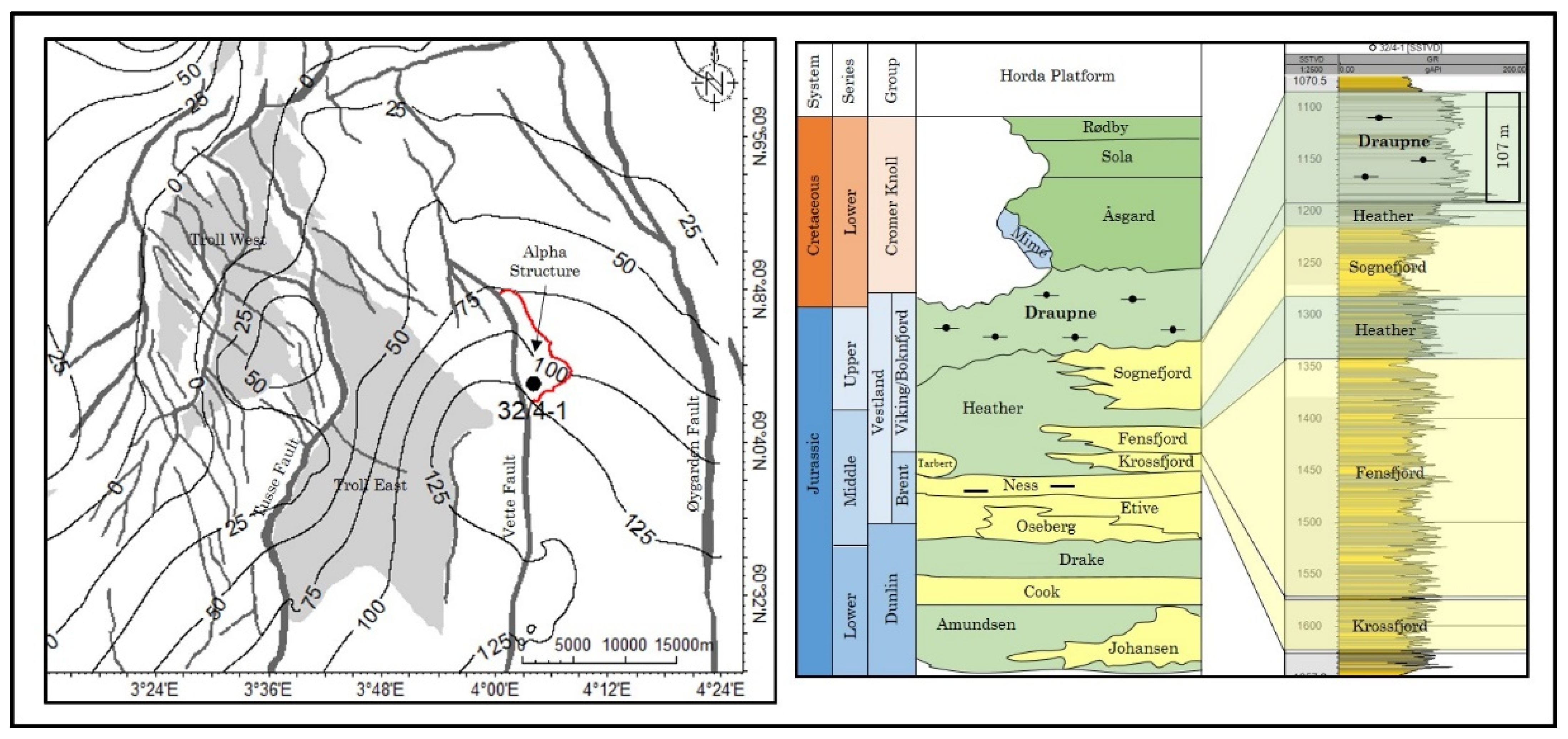Therefore, the caprock reliability assessment is necessary to prevent any CO₂ injection-related leakage risk. The Alpha prospect is a fault-bounded three-way structural closure located in the Smeaheia area, northern North Sea (Figure 1). The Alpha prospect was evaluated by Equinor and Gassonova as a potential CO₂ storage site [14]. The area is located east of the Troll east field and bounded by two major faults; Vette Fault (VF) in the west and Øygarden Fault Complex (ØFC) in the east. The studied site is positioned in the footwall of the VF with a three-way closure [15]. The main reservoir rocks comprise Upper Jurassic Sognefjord, Fensfjord, and Krossfjord formations, while the organic-rich Draupne and Heather shales act as the primary caprocks.

The abundance of fine-grain particles (i.e., clay minerals) in the Draupne shale [15] has indicated that it is unlikely to have a capillary breakthrough. Hence, the main top-seal failure is related to mechanical stability. However, the estimation of caprock mechanical properties is very complex and uncertain. Moreover, how the injection-related horizontal stress path changes are mostly unknown in a saline aquifer. Additionally, due to the lack of core samples of Draupne and Heather shale caprocks, laboratory-derived rock strength properties have limitations, which add more uncertainties. Deterministic caprock assessment is somewhat questionable when a significant number of uncertain parameters are present [17]. Instead, a stochastic approach might be more fruitful [18,19].

Machine learning (ML) algorithms are a category of models that can detect patterns and deduce the underlying mathematical relationships without prior knowledge. To make predictions or judgments, they create a mathematical model based on sample data, known as training data. ML techniques have recently shown promising performance in solving geoscience-related problems [20,21,22].

For example, injecting CO₂ into abandoned oil fields disrupts the reservoir field pressure, which may result in leakage. Harmonic pulse testing (HPT) is a technique used in field testing to identify the pressure response of a leak from that of a non-leak. In a CO₂ capture and storage (CCS) project, CO₂ potentially may leak from numerous injection wells and depleted wells. Since human analysis of vast amounts of HPT data is challenging, ML approaches are viable alternatives. In this regard, Sinha et al. [23,24] predicted CO₂ leakage using a variety of NN approaches such as multilayer NN, convolutional neural network (CNN) and long-short term memory (LSTM). Sun et al. [25] used a NN technique to investigate the CO₂ trapping mechanisms in the Morrow B Sandstone in the Farnsworth Units. In light of the NN forecasts, they picked the reservoir model from an available historical data. The chosen model then was used to assess the effect of the structural-stratigraphic mineral trapping mechanisms on CO₂ sequestration. Furthermore, the NN-based model was capable of accurately predicting pressure, fluid saturation, and composition distributions. As a result, they concluded that mineral trapping contributes less to CO₂ sequestration than other trapping methods. Lima and Lin [26] predicted CO₂ and brine leaks in a GCS project using ml algorithms. They used seismic data and historical well pressure data from 500 simulations as inputs to the CNN model. Testing the model, 50 out 500 simulation data were used as the test data. They observed incorporating the pressure data gives a slight improvement in leakage prediction as well as increasing prediction accuracy. To predict CO₂ leakage, Zhong et al. [26] employed a combined version of CNN and LSTM model (ConvLSTM). They employed CNN and LSTM to handle spatial features (porosity and permeability) and temporal features (CO₂ injection rate per time), respectively. In other words, three 2D images were utilized as input to convLSTM, one of which included the injection rate and the other two were porosity and permeability distributions.

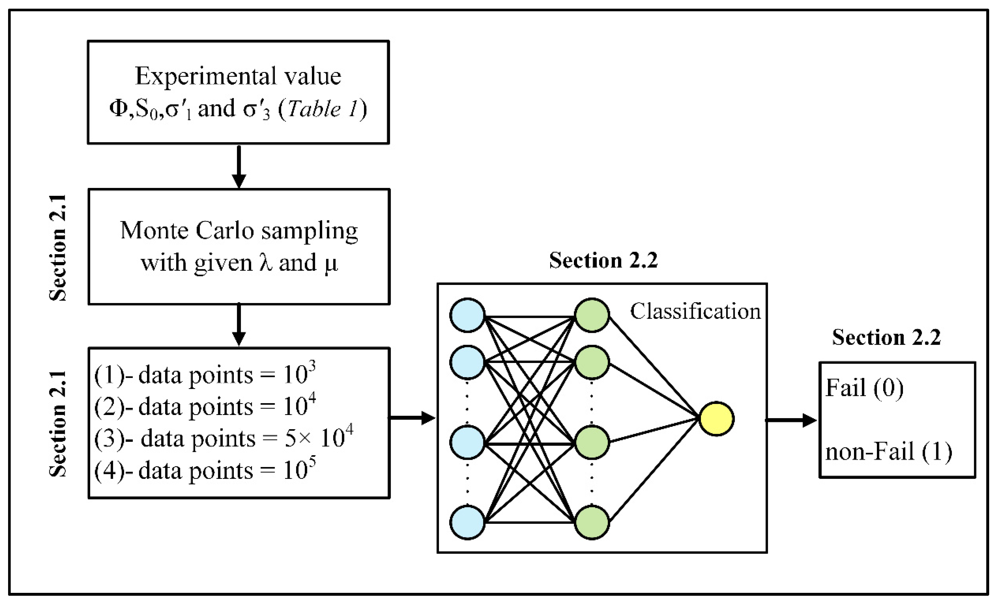
In this study, the Monte-Carlo (MC) algorithm is used to produce stochastic rock strength parameters based on given average and variance. Then, stochastic reliability analysis (SRA) is employed to predict the factor of safety (FoS) of each realization. Following the completion of a limited number of Monte-Carlo simulations and the acquisition of FoSs, the data are introduced into the NN model as training data to find a general prediction for FoS without the need for Monte-Carlo simulation. To validate the effect of the number of realizations on FoS prediction, different sizes of sample data were introduced to establish NN as the test data.

2. Theoretical Background

This section discusses the theoretical principles in detail. Section 2.1 describes the Monte Carlo sampling algorithm based on the given mean value and standard deviation. Section 2.2 delves further into the concepts of machine learning and neural network for binary classification. The study’s workflow is depicted in Figure 2.

2.1. Monte Carlo Simulations

Monte Carlo-based statistical methods have shown promising potential in generating stochastic input parameters from available lab measurements. The MC algorithm was used in conjunction with the Gaussian formalism to estimate the strength parameters of cohesion (S₀) and friction angle (φ) and effective stresses (i.e., σ’₁, and σ’₃). In this approach, the given mean value, and standard deviation were substituted into Gaussian formalism at each MC step. In other words, replacing the mean value and variance in Equation (1) with relevant values (introduced in

Table 1. The used database, including mean value (λ) and standard deviation (μ) of strength parameters (φ and S₀) and effective stresses (σ’₁ and σ’₃) [16].

Parameters	Mean Value (λ)	Standard Deviation (μ)	Unit	Distribution	Sample Number
Φ	19.50	3	Degree	Normal	* Lab + Logs (429)
S0	5.01	1	MPa	Normal	** XLOT (5)
σ’1	22.25	0.55	MPa	Normal	Lab + Logs (432)
σ’3	16.85	0.7	MPa	Normal	Lab (4)

* Lab, laboratory analysis; ** XLOT, extended leak-off test.

) allow having a Gaussian distribution from stochastic values for φ, S₀, σ’₁, and σ’₃.

$$f(x,\mu ,\lambda )=\frac{1}{\sqrt{2\pi \lambda }}{\mathrm{e}}^{\frac{{}^{-{\left(x-\mu \right)}^2}}{2{\lambda }^2}}$$

(1)

Equation (1) represents the Gaussian distribution formula, where λ is the mean value and μ is the standard deviation and form bell shape plot displaying the normal distribution of independent variable x.

Model Definition

The caprock shale structural reliability depends on the stresses (i.e., σ₁, σ₃) and rock strength properties (i.e., S₀, φ). These parameters act as load and resistance, which allow estimating failure probability with evaluating the safety margin. This context tests the Mohr-Coulomb failure criteria based on the factor of safety (FoS). Equation (2) is used to determine the factor of safety (FoS) by estimating the φ, S₀, σ’₁, and σ’₃ in combination with the MC algorithm.

$$FoS=\left(\frac{2}{{\sigma }_1^{\prime }-{\sigma }_3^{\prime }}\right)\left[\left(\frac{{\sigma }_1^{\prime }+{\sigma }_3^{\prime }}{2}\right)+\frac{S_0}{\tan \left(\phi \right)}\right]\sin \left(\phi \right)$$

(2)

where S₀ is cohesion, φ is friction angle, σ’₁ is effective vertical stress, and σ’₃ is effective horizontal stress. The effective stresses are estimated from reservoir pore pressure (p_p) following Equations (3) and (4).

$${\sigma }_1^{\prime }={\sigma }_1-p_p$$

(3)

$${\sigma }_3^{\prime }={\sigma }_3-p_p$$

(4)

The p_p in Equations (3) and (4) are pore pressure, which is considered 10.48 MPa [16]. For simplicity, the model has assumed an isotropic horizontal stress condition with a normal faulting regime. The deterministic FoS values are estimated using the stochastic data generated by MC algorithm. Afterward, the number of failures (FoS ≤ 0) and non-failure (FoS > 0) states are counted to estimate the failure percentages of caprock shales.

2.2. Machine Learning

Machine learning (ML) is a data analysis approach that automates the construction of analytical models. The principle that computers can learn from data and discover the data patterns without explicit human intervention has been constructed on ML algorithms. In order to build an ML-inspired mathematical model, the sample data is initially classified into train and test categories. The train data set is used to fit a model, while the test data set is utilized to evaluate the performance of the model in prediction (regression) or decision making (classification). Here, it is supposed to discover the mathematical correlation between FoS and input data with ML algorithm. In this regard, by feeding the train data set calculated with MC simulations into ML algorithm, the mathematical correlation between g(x) and input parameters (φ, S₀, σ’₁, and σ’₃) will be discovered with the ML algorithm. Afterward, with introducing the test dataset to the trained-ML algorithm, the corresponding g(x) will be predicted. Several ML algorithms have been developed, such as Bayesian network, neural network, decision tree, random forest, etc. In this simulation, the potential of the neural network (NN) has been investigated.

2.2.1. Neural Network

The artificial neurons model was initially developed by McCulloch and Pitts [27] in 1943 to explore signal processing in the brain, and it has since been improved by others. The main concept is to imitate biological neural networks (NN) in the human brain, which are mainly composed of billions of neurons that communicate by transmitting electrical signals to one another. To produce an output, each neuron collects receiving signals, which must surpass an activation threshold. If the threshold is not crossed, the neuron stays dormant (inactive), producing no output. The mentioned behavior has sparked the development of a basic mathematical model for an artificial neuron. Equation (5) represents the output of a neuron that receives weighted sum signals x₁,…, x_n as input from N neurons.

$$y=f\left({\displaystyle \sum _{i=1}^N{w}_i{x}_i}\right)$$

(5)

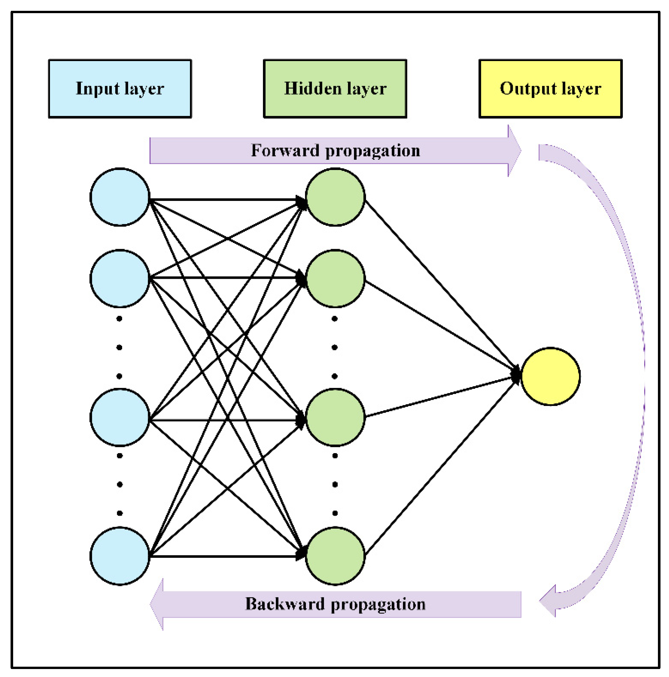
Artificial neural network (ANN) in the form of machine learning is a computational paradigm that is made up of layers of linked neurons, also known as nodes. In order to imitate a biological neural system, each neuron interacts with other neurons by transmitting mathematical functions across layers [28]. The main architecture of ANN is comprised of an input layer, an output layer, and eventual layers in between called hidden layers. Each layer includes an arbitrary number of nodes, and each connection between two nodes is defined with an associated weight variable. The weights (signals) are real numbers multiplied by a node’s internal state to create a weighted sum and transmit from the input layer to the output layer. By summing the weight transformations of a layer, a propagation function may be created to determine the input to a node from the outputs of its previous node. NN uses activation functions for hidden layers, which are non-linear, bounded monotonically increasing, and continuous functions.

2.2.2. Mathematical Description of NN

In order to implement a multilayer NN for the first hidden layer, the weighted sum is written as represented in Equation (6):

$$y_i^1=f\left(z_i^1\right)=f\left({\displaystyle \sum _{j=1}^{N_0}{w}_{ij}^1{x}_j+b_i^1}\right)$$

(6)

where y is output from the first layer, z is the weighted sum, f is the activation function, i is the number of neurons at the first layer, the superscript 1 shows the first hidden layer, b is biased, and N₀ is the number of nodes in the first layer. For the l-th hidden layer, we have:

$$y_i^l=f^l\left({\displaystyle \sum _{j=1}^{N_{l-1}}{w}_{ij}^l{y}_i^{l-1}+b_i^l}\right)$$

(7)

In Equation (7), the superscript l, shows different active functions (f^l) are used for each layer. The closed form of forward propagation for a multilayer NN is written as:

$$y_i^{l+1}=f^{l+1}\left[{\displaystyle \sum _{j=1}^{N_l}{w}_{ij}^3{f}^l\left({\displaystyle \sum _{k=1}^{N_{l-1}}{w}_{jk}^{l-1}\left(\dots f^1\left({\displaystyle \sum _{n=1}^{N_0}{w}_{mn}^1{x}_n+b_m^1}\right)\dots \right)+b_k^2}\right)}+b_1^3\right]$$

(8)

As seen in the forward propagation algorithm, the weights are added up from the previous layer, and after combining with the activation function, move toward the output layer. It is possible to rewrite a compact version of Equation (8) by showing the weight, bias, and y in vector format.

$$y_i^l=f^l\left(W^l{\stackrel{⌢}{y}}^{l-1}+{\stackrel{⌢}{b}}^l\right)$$

(9)

Here W is the weight vector with a dimension of N_l−1 × N_l while $\stackrel{⌢}{y}$ and $\stackrel{⌢}{b}$ are output and bias vectors with a dimension of N_l × 1, which are shown layer-wise. In Equation (9), the unknown parameters are biases and weights, which can be tuned to diminish the error of the NN model. The backpropagation algorithm [29] allows tuning of weights and biases by minimizing the cost function.

$$C(\stackrel{⌢}{W})=\frac{1}{2}{{\displaystyle \sum _{i=1}^n\left(y_i-t_i\right)}}^2$$

(10)

Equation (10) represents the cost function. As seen in Equation (10), $\stackrel{⌢}{t}$ is a vector of target values and $\stackrel{⌢}{y}$ is an output of neural network (NN) showing in vector format. In other words, forward propagation of the $\stackrel{⌢}{x}$ into NN gives $\stackrel{⌢}{y}$. Equation (11) is introduced for the back propagation algorithm, which calculates ${\stackrel{⌢}{a}}^{l-1}=f\left({\stackrel{⌢}{z}}^l\right)$ and then plugged it into the last hidden layer as an input.

$${\stackrel{⌢}{z}}^l={\left({\stackrel{⌢}{W}}^l\right)}^T{\stackrel{⌢}{a}}^{l-1}+{\stackrel{⌢}{b}}^l$$

(11)

The new argument of activation function (${\stackrel{⌢}{z}}^l$) will be updated by modified ${({\stackrel{⌢}{W}}^l)}^T$ and ${\stackrel{⌢}{b}}^l$. The value of cost function, introduced in Equation (12), is optimized by propagating from output toward the input layer by modified weights and biases. Learning is a method of adjusting the weights and biases in order to minimize the cost function and increase accuracy. Although no specific criteria are provided into the NN for analysis, the NN is able to develop its own logic after training with the train data set. To implement the NN, the network architecture should first be derived: the number of layers, type of NN layers, number of nodes, and activation functions. Secondly, the network is trained on train data. After training, the model architecture is saved along with the final weights for each neuron. Finally, the trained model can be applied to unseen data (i.e., the test data set). By applying the NN to the test data set, the weights in the architecture network are fixed and are not allowed to be optimized anymore. The sketch in Figure 3 depicts the overall architecture of a classification (NN), including the forward and backward propagation algorithms.

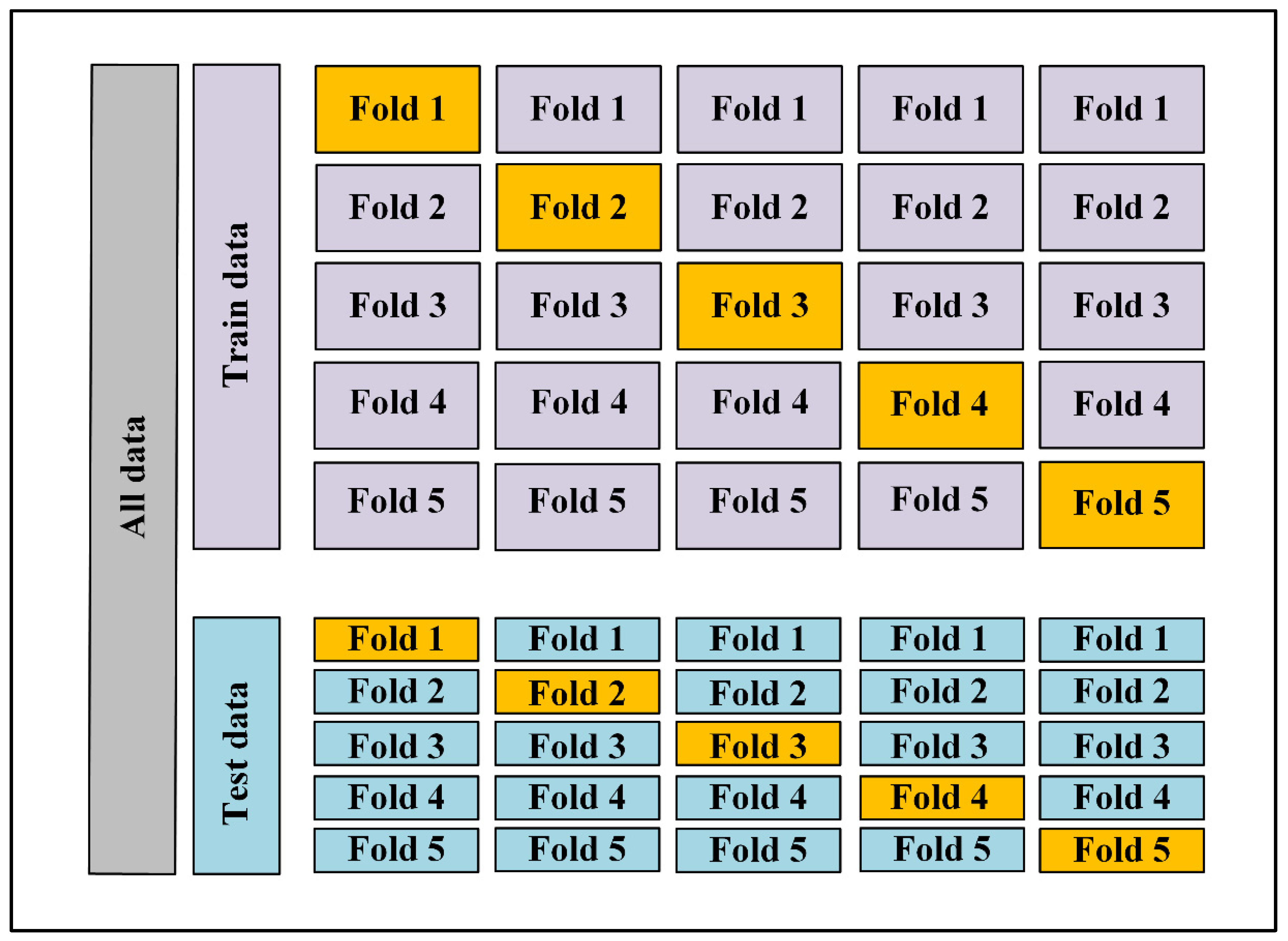
2.3. K-Fold Cross-Validation

The established NN model was combined with the 10-fold cross-validation algorithm. The k-fold cross-validation method applies to both train and test data sets, such that the original data set is randomly divided into k equal-sized subsamples (fold) several times. One subsample is chosen for validation while the k-1 folds are utilized for training. Then, the model’s performance metrics will be averaged across several runs. The k-fold cross validation has the advantage that every subsample (in the train and test datasets) contributes to training and validation, and each fold is only used for validation once. Figure 4 depicts graphically how the train and test data sets are organized using 5-fold cross-validation.

3. NN Model Implementation

Due to a scarcity of caprock cores, very few laboratory-tested rock strength properties are available in the studied area. Besides, owing to a large number of uncertainties, the probabilistic approach is more convenient for caprock integrity than the deterministic approach [17,18,19].

To do this, the mean and standard deviation values from Table 1 were substituted into Equation (1) at each MC cycle. Initially, MC simulation produces four separate data sets of different sizes: 1000, 10,000, 50,000, and 100,000 data points for each φ, S₀, σ’₁, and σ’₃. The resulting MC data were then merged with pertinent g(x) values in a unique matrix to create input data sets with the size of 1000, 10,000, 50,000, and 100,000. The NN conjugated with a 10-fold cross-validation algorithm is developed to establish an ML model that can predict the proper g(x). Hereafter, the term “NN model” refers to a neural network combined with the 10-fold cross-validation algorithm. The NN with a simple architecture is designed via trial and error to minimize training time. Three layers of the NN model are proven to be sufficient to achieve a satisfactory outcome (14 nodes initial layer, 10 nodes second layer, and 1 node final layer) with a dropout rate of 20% to prevent overfitting. The last layer was activated using the sigmoid function, whereas the other layers utilized the rectified linear unit (ReLU) [30] activation function. In the NN model, each input data set contains four features (φ, S₀, σ’₁, and σ’₃), as well as a target g(x) which may be either one (indicating non-Fail) or zero (showing Fail). 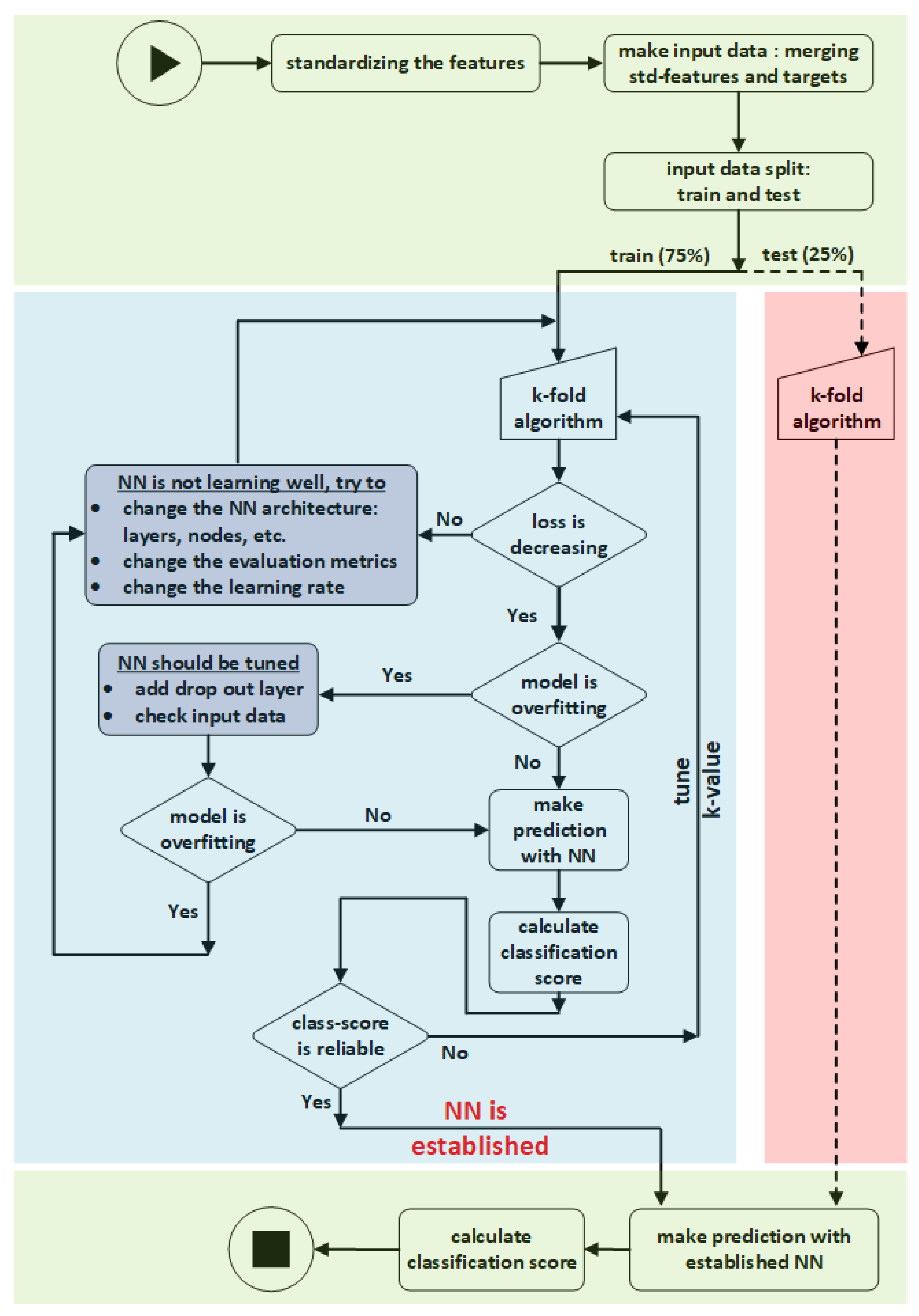Figure 5 illustrates the flowchart of NN establishment with train dataset and then validation with test dataset. The input data is split into train and test datasets before being fed to NN. The training dataset is necessary to fit the NN model, whereas the test dataset is utilized to evaluate the error of the model predictions. Here, the input dataset is divided into train and test datasets, with a percentage of 75% for training and 25% for testing.

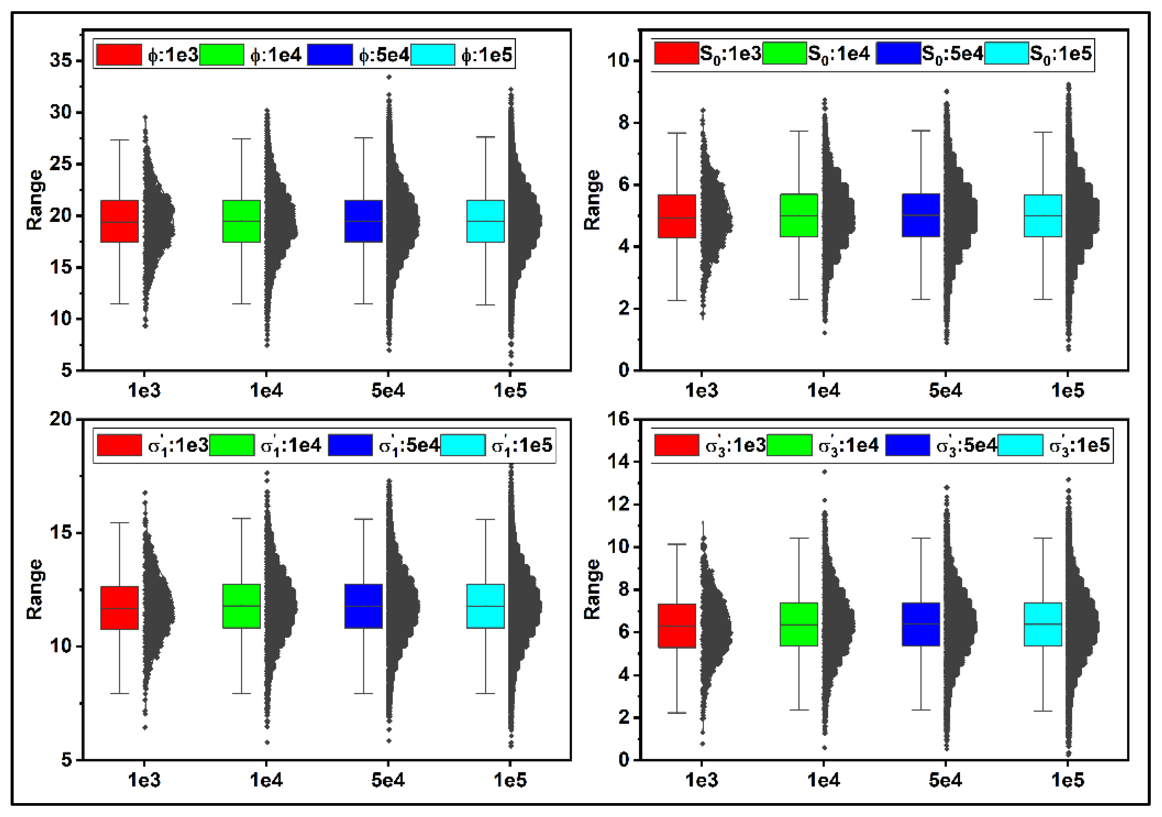
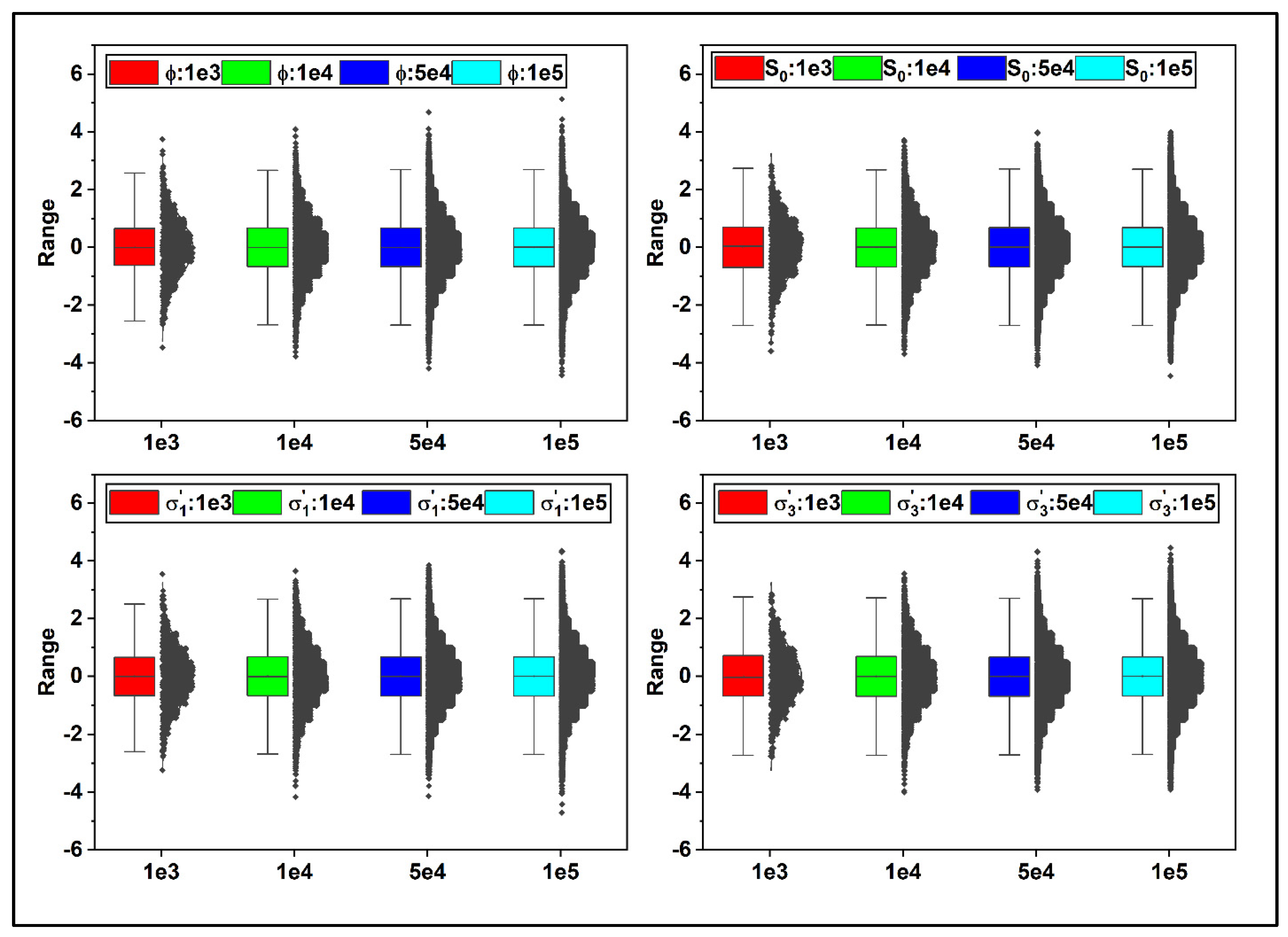
Figure 6 represents the probability distribution function (PDF) of ϕ, S₀, σ’₁, and σ’₃ for different sample sizes. As seen, the PDF diagram behaves identically for various sample sizes, even though the depicted ranges vary by sample size. In other words, regardless of sample size, the mean value and standard deviation of each curve shown in Figure 6 are the same as those given in Table 1.

3.1. Input Data Scaling

Scaling, often known as standardization, is a data pre-processing task that applies to the features. Scaling not only aids in the normalization of data within a specific range it may also aid in the speeding up of computations in an algorithm. The reason for standardization is the units of input variables may vary, implying that the variables have distinct scale units. The scale unit differences among input variables increase the complexity of the model since large input values may lead to a model with large-weight values. A large-weight model is unstable due to poor results in training and increases the sensitivity to input values, consequently generating significant errors. Figure 7 shows the distribution of the input values to ML algorithm after standardization. The standardization approach in Figure 7 involves subtracting λ from each data and dividing it by μ. As seen in Figure 7, scaling preserves the original data distribution structure while enabling each data distribution to have a mean of zero and a standard deviation of one, thus speeding up the NN algorithm’s calculations.

3.2. NN Verification

In order to verify the designed NN, it is required to evaluate the performance algorithm with the contrived datasets. These datasets have well-defined characteristics that allow exploring a specific algorithm behavior. The scikit-learn library provides make-moons and make-circles data set that suites verifying the classification algorithms. To include the make-moons data set in our network, 1e+03, 1e+04, 5e+04, and 1e+05 data generated and then split into the train (75%) and test (25%) datasets. First, the training dataset was introduced to NN to fit a model for the dataset. Then, the performance of the fitted model was examined against the test dataset. Figure 8 shows the trend of the fitting score and fitting time for make-moons and make-circles data set. As shown, for the train data, the fitting score starts at 0.92 and lays on 0.94 at the end. Simultaneously, for the test data, the trend of the fitting score ascends when the size of the input dataset increases from 1e+03 to 1e+05. In addition, the fitting time has ascending regime by increasing the input data size, which is consistent with our expectation. The verification results shown in Figure 8 demonstrate the efficiency of the NN model for classification. Therefore, in the next step the NN model is applied for the classification of the real input dataset.

3.3. Metrics for Evaluating the NN Model

The Adam stochastic optimizer [31] was applied as a metric to monitor the convergence progress of the established NN. The reason is that choosing the learning rate is not easy since the network approaches a local minimum with high learning rates, causing instability in the training process. On the other hand, low learning rates are computationally costly since they extend the learning process. However, the Adam stochastic optimizer has adaptive learning rates that optimize stochastic objective functions by repeatedly updating network weights. Cross-entropy was used to estimate the loss function. As the loss function defines the network’s objective throughout the training, the cross-entropy function has been selected to minimize the gap between probabilities. The accuracy metric also was selected in conjunction with cross-entropy to capture the convergence progress of the loss function.

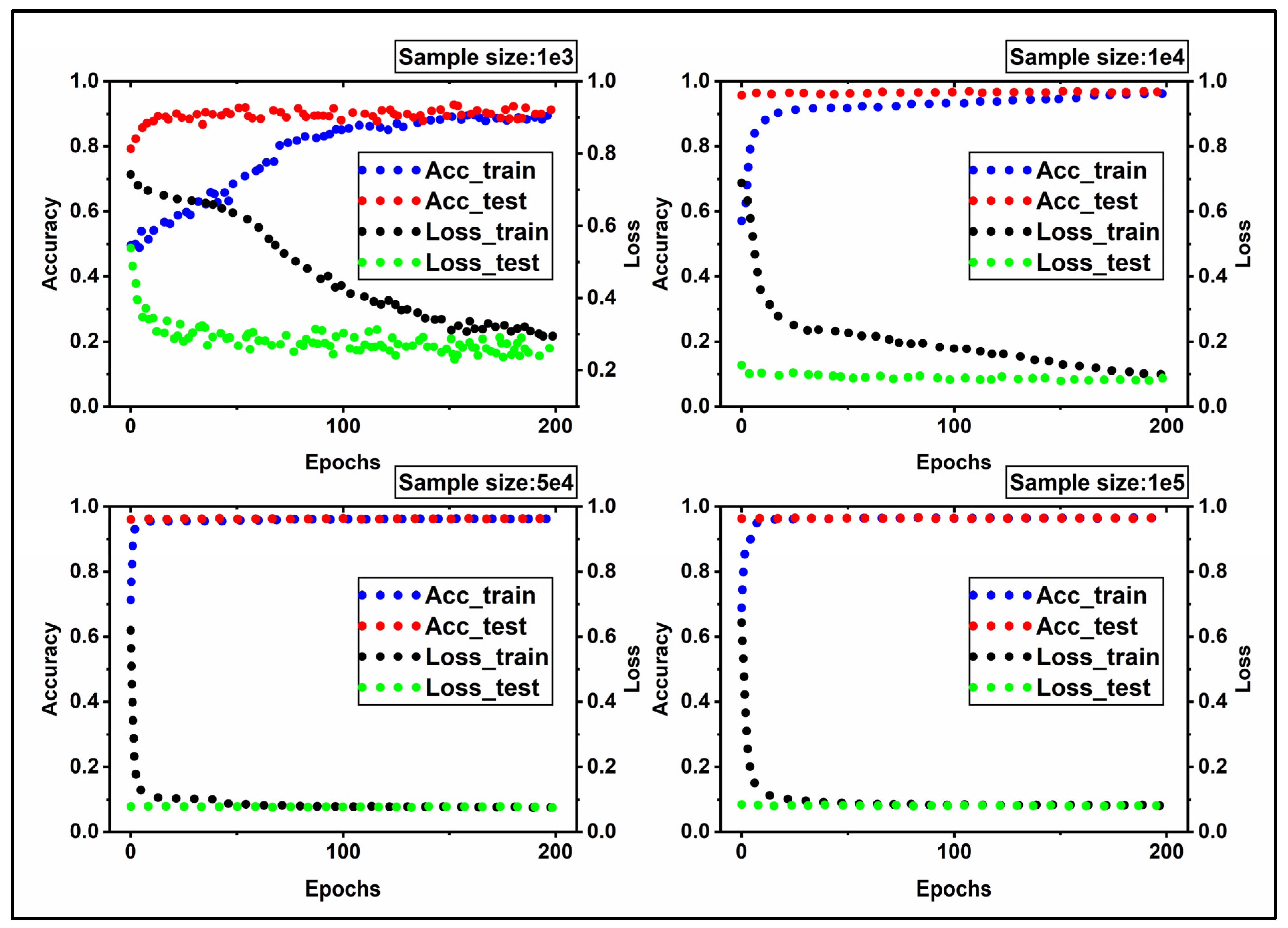
To investigate the impact of data size on the training process of NN, we introduced various sizes of input data to NN using the same metrics and epochs.

Figure 9 shows the trend of accuracy and loss functions for train and test datasets. The ascending and descending profile for accuracy and loss in Figure 9 shows the NN learns appropriately. However, the distinct behavior of NN with various input datasets produced a unique pattern for each input data size. Although the input datasets after scaling have a mean value of zero and a standard deviation of 1, they differ in size. In Figure 9, the blue and red circles depict the accuracy profile for train and test data sets, respectively, while the black and green circles depict the loss function profile for train and test data sets. When epochs = 160, the loss function of train data stabilizes at about 0.2 for input data of size 1e+03, whereas the trend for 1e+04 first declines and eventually stabilizes around 0.1 when epochs = 200. When the size reaches 5e+04 and 1e+05, the loss profile significantly decreases and stabilizes around 0.07 and 0.06, respectively. Simultaneously, the accuracy trends increase significantly and settle at 0.99. In comparison to 5e+04 and 1e+05, inputs of size 1e+03 and 1e+04 provide less accuracy. In other words, shifting from 1e+03 data to 1e+04, 5e+04, and 1e+05 data improves convergence conditions, resulting in higher accuracy and smaller loss. He et al. [32] also, had reported a larger sample size leads to a higher accuracy. The accuracy and loss profiles for test data sets, including all available data sizes, exhibit more favorable convergence conditions than train data sets.

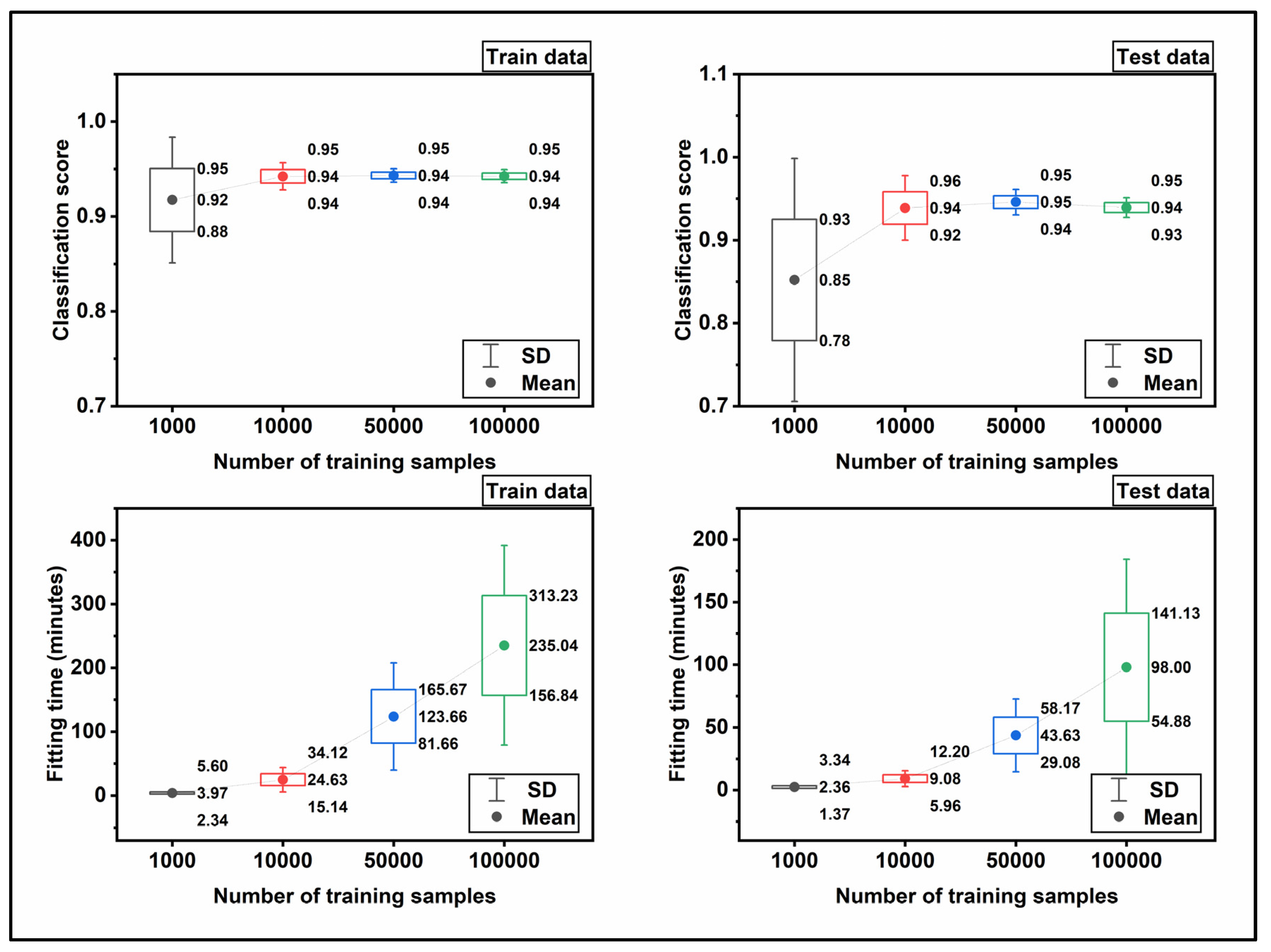
In order to measure the classification performance quantitatively, a function is employed to measure the ratio of True predictions over all possible forecasts. For instance, in our case, there were four possible predictions: True Fail, False Fail, True non-Fail, and False non-Fail. Therefore, the classification score is calculated as:

$$\mathrm{classification}\hspace{0.17em}\hspace{0.17em}\mathrm{score}\hspace{0.17em}=\hspace{0.17em}\frac{\mathrm{True}\hspace{0.17em}(\mathrm{Fail})\hspace{0.17em}+\hspace{0.17em}\mathrm{True}\hspace{0.17em}(\mathrm{non}-\mathrm{Fail})}{\mathrm{True}\hspace{0.17em}(\mathrm{Fail})\hspace{0.17em}+\hspace{0.17em}\mathrm{False}\hspace{0.17em}(\mathrm{Fail})+\mathrm{True}\hspace{0.17em}(\mathrm{non}-\mathrm{Fail})+\mathrm{True}\hspace{0.17em}(\mathrm{non}-\mathrm{Fail})}$$

(12)

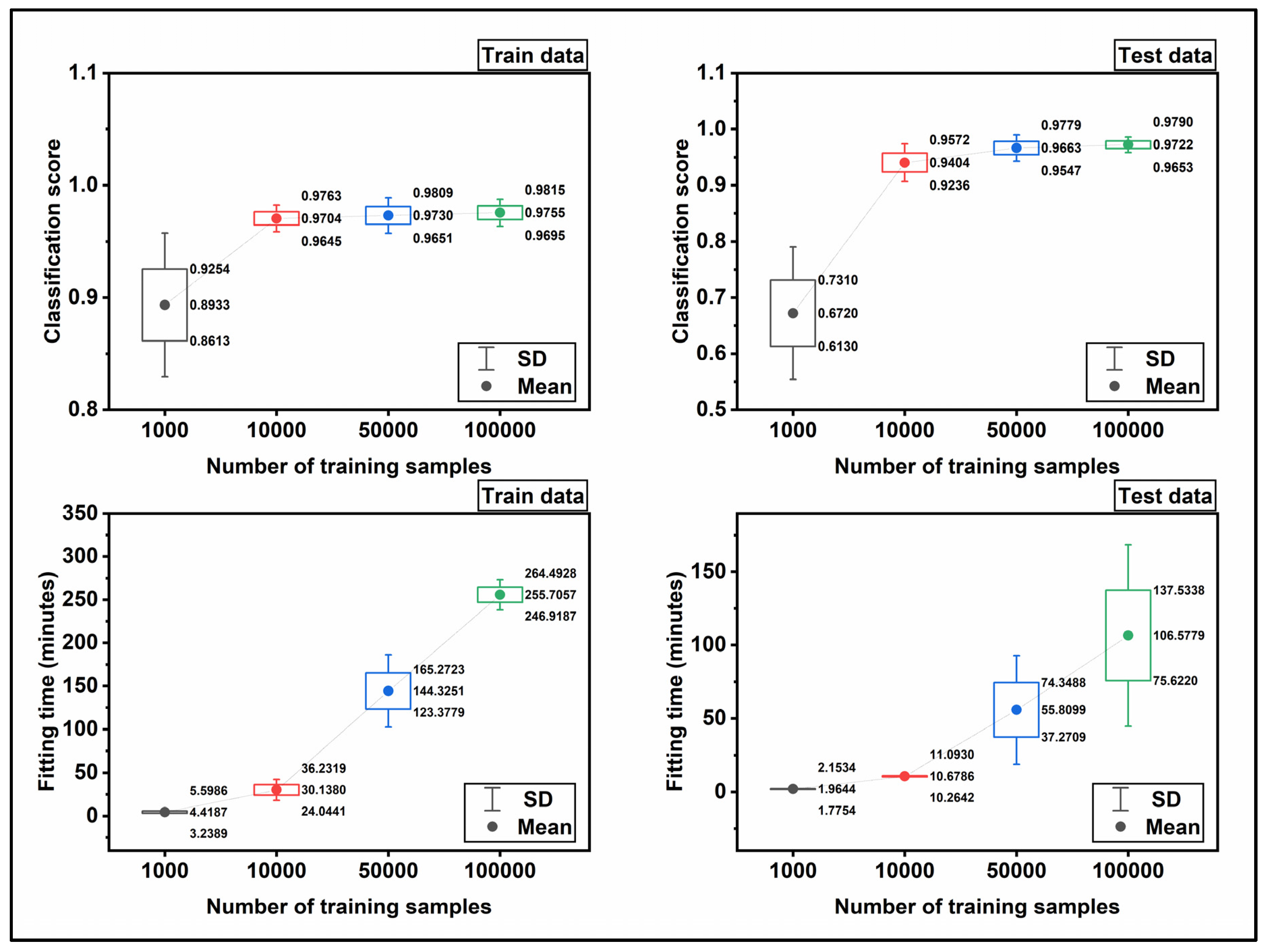
Figure 10 displays the trend of the classification scores and fitting time for the train and test datasets. The mean values and standard deviations were plotted with filled circles and error bars, respectively. The classification scores in Figure 10 were calculated based on the fraction mentioned above. Namely, to calculate the mean value for the classification score, the score is averaged for 10-fold cross-validation, and the relevant standard deviation was determined simultaneously. As observed, the classification score for train and test data increases when the size of the input data increases. To be specific, from 1000 to 10,000 a sever slope is observed in classification score while the trend stabilizes approximately after 50,000 to 100,000. For train data, the mean score starts with 0.89 for the 1e+03 input data and reaches 0.98 for the 1e+05 input data. The same trend is observed for test data, and the main difference is the kick of score for the 1e+03 data, which is 0.67. The fitting time is depicted in Figure 9, is also averaged over 10-fold cross-validation. As seen, the fitting time increases by increasing the size of the input data.

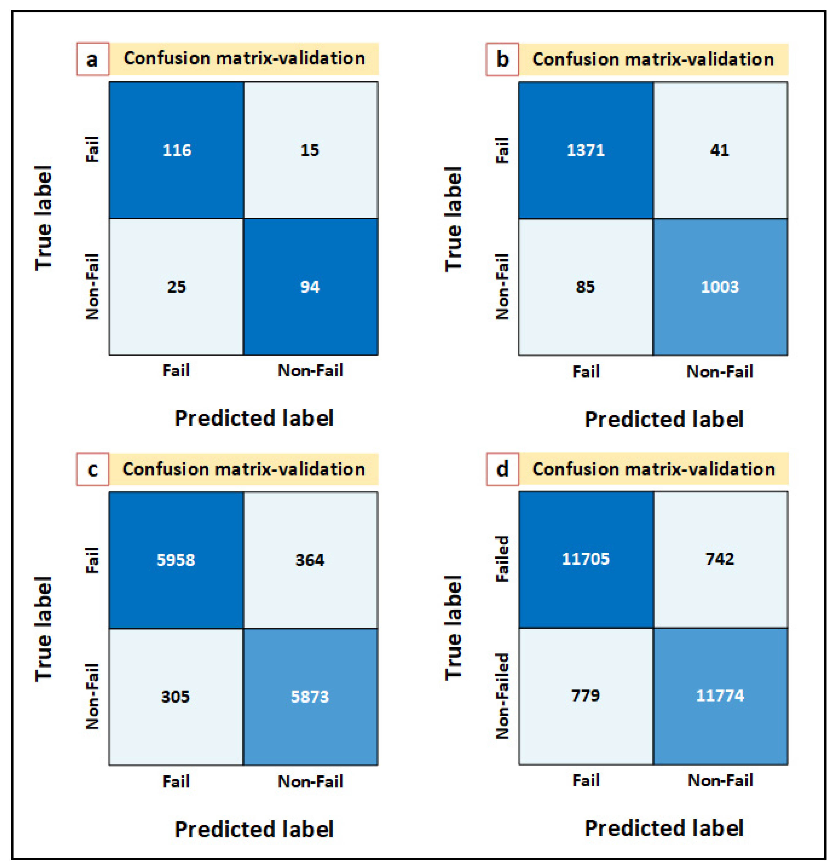
In order to validate the NN model, it is necessary to feed the model with an unseen data and assess the outcomes. To that end, unseen data points of 250, 2500, 12,500 and 25,000 are introduced into the NN model. The validation results for 250, 2500, 12,500, and 25,000 unseen data are shown in Figure 11a–d.

4. Alpha Site Case Study

Alpha prospect is a potential site for a long-term CO₂ storage located in Horda Platform, northern North Sea (Figure 1). It is critical to evaluate the structural reliability of the sealing effectiveness (i.e., caprock and fault) at the Alpha structure since it is a three-way closure against fault. In this study, the strength parameters are initially developed using MC algorithm as this approach was already employed by He et al. [32] to obtain the FOS variables. On the other hand, Wang and Goh [33] previously generated FOS parameters using random field finite (FE) element method. Here, MC generated strength parameters were then fed into NN model to assess the Draupne Formation shale caprock probabilistic failure potential. While He et al. [32] chose NN along with support vector regression, Wang and Goh [33] employed CNN approach in their study. However, the database used in this study is only limited to the Alpha prospect (well 32/4-1) without considering the spatial properties variation [15]. This includes additional constrained of the sampling method. Significantly good classification results in machine learning algorithms instill confidence in our capacity to evaluate field scale dependability using the NN model. However, in 1000 data samples, the small input data size has limited results and is not trustworthy. Therefore, the results of the 1000 data samples were excluded from

Table 2. Predictions made by the developed NN versus test data samples. It is worth mentioning that the test dataset used to validate the NN model represents 25% of total data samples.

Number of Total Test Data	Number of Correct Predictions	Non-Fail	Fail	Classification Score
2500	2374	43%	57%	94%
12,500	12,131	42%	58%	97%
25,000	24,311	42%	58%	97%

. In other words, the reported results in Table 2 corresponds to the models with 10,000, 50,000, and 100,000 data samples. As seen in Table 2, as the sample size grew, the classification score climbed to 94%, 97%, and >97%, respectively. As mentioned before, this fact was already reported by He et al. [32]. It is worth mentioning that the test dataset used to validate the NN model represents 25% of total data samples, while the remaining data (i.e., 75%) is utilized for training the NN model. As shown in Table 2, the developed NN predicts that more than 50% of test data results will be in the failure state, which is significantly overestimation compare with the results estimated using other method [34]. As previously stated, the absence of experimental data may introduce substantial uncertainty into the presented findings. Moreover, subsurface structural reliability is a delicate procedure that is influenced by a variety of other parameters. Therefore, further comprehensive investigation is required to evaluate the critical top seal integrity for a safe and reliable subsurface CO₂ storage in the Alpha prospect.

5. Conclusions

The reliability of the NN method for the caprock shale integrity prediction was investigated. The critical observations of this study are as follows:

• By increasing the size of the input data, the developed NN converges at shorter epochs.
• The classification score rises as the size of the input data increases and almost stabilizes after 50,000 data samples.
• The NN algorithms are feasible alternatives to time-consuming finite element techniques in terms of computing time. In other words, although the fitting time increases with increasing the input data size, it is still negligible when compared to conventional methods.
• Although the NN method tested in this study shows significantly high classification score, the Draupne caprock shale probabilistic failure significantly overestimated the failure potential. However, owing to a scarcity of experimental data and complex caprock behavior, additional field investigation and empirical evidence are required to predict the more definite failure state.

This study indicated the practicality of the machine learning technique in caprock structural reliability analysis. However, ML methods sometimes limited by factors such as lack of physical constraint, data availability and quality. In addition, the subsurface caprock laboratory data has limitation itself. Therefore, we need to investigate further to increase our confidence on field scale caprock integrity. Moreover, injection induced pressure change in any CCS projects need to be investigated which potentially could be future study.