Abstract
The publication presents the results of research on soil temperature distribution at a depth of 0.25–3 m in three measurement locations. Two boreholes were located in Białystok in the temperate climatic zone and one measuring well was installed in Belmez in the subtropical climatic zone. Measurements were made in homogeneous soil layers in sand (Białystok) and in clay (Białystok and Belmez). Based on the results of the measurements, a simplified model of temperature distributions as a function of depth and the number of days in a year was developed. The presented model can be used as a boundary condition to determine heat losses of district heating pipes located in the ground and to estimate the thermal efficiency of horizontal heat exchangers in very low-temperature geothermal energy applications.
1. Introduction
Research on temperature distributions in the ground is most often carried out in terms of vertical or horizontal heat exchangers associated with heat pumps. Sliwa et al. [1] developed a methodology for determining the energy efficiency of borehole heat exchangers based on temperature profiling. In the case of vertical heat exchangers, the ground temperature distributions concern considerable depths as a function of the length of the boreholes [2,3,4,5,6,7]. Horizontal ground heat exchangers usually require knowledge of temperature distributions in the ground up to several meters [8,9,10,11,12]. The knowledge of temperature distributions in the ground is the basic boundary condition for designing underground heating pipes. In designing district heating networks, the most common methods are calculation methods, in which a constant average annual ground temperature is assumed [13,14,15,16,17]. In the case of recreating the actual operating conditions of the pre-insulated networks, the actual ground temperatures should be set. An example of the location of pipes in district heating in Poland is shown in Figure 1. In the case of two- and three-dimensional calculations, the soil temperature at the assumed depth is determined for the boundary temperature condition at the depth of 8 m, equal to 8 °C [18,19,20].
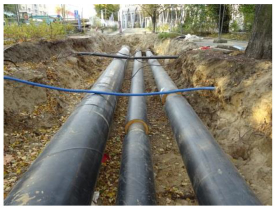
Figure 1.
Example of pre-insulated heating pipes located in the ground layer at a depth of up to 1 m.
Temperature distributions in the ground can also be useful for determining heat losses in fermentation chambers of biogas plants, if the fermentation chambers are immersed in the ground [21,22,23].
There are many models of temperature distribution in the ground in the literature. Models of temperature distribution in the ground are very often described with the dependence of air temperature or parameters of solar radiation [24,25,26,27]. In [24], the Carslaw and Jaeger equation [28] was used for the modeling of soil temperature and demonstrated a significant influence of solar radiation on the soil temperature. The Carslaw and Jaeger equation [28] can also be used in mathematical modeling of a horizontal ground heat exchanger [25]. In [26], the McAdams [29] and Kusuma [30] correlations describing the convective heat exchange between the flowing wind and the ground surface were used in the model of heat exchange in the ground. The publication [27] presents the methods of calculating the undisturbed ground temperature on the basis of the heat flux balance and meteorological data averaged over the yearly cycle. In some regions with rainy weather, it is crucial to take into account relative humidity and rain duration and their impact on the sub-soil temperature profiles, as shown by Molina-Rodea and Wong-Loya [31].
Most of the known models of temperature distribution in the ground down to a depth of several meters depend on meteorological data and require access to these data. In the case of designing horizontal ground heat exchangers, pre-insulated heating networks, or thermal insulation of walls of recessed digesters, simplified algorithms of temperature distributions in the ground as a function of days a year, which could be included in industry standards or design guidelines, are sufficient. The simplest solution is to develop a model of temperature distribution in the ground based on the measured temperatures in the ground over a two-year period for a given type of soil and selected location. The aim of the work is to investigate the temperature distribution in the ground layer at a depth of 0.05–3.00 m and to develop a simplified model of temperature distribution in the ground layer where heating pipes and horizontal heat exchangers can be located. Ground temperature measurements were made for two points in a temperate climate and one point in a subtropical climate. No simplified models of temperature distribution in the ground for the assumed locations have been found in the literature.
2. Materials and Methods
The study of temperature distribution in the ground was carried out in selected locations in a temperate and subtropical climate. In a temperate climate, measurements were made in north-eastern Poland in the suburbs of the city of Bialystok, while in a subtropical climate, measurements were made in the city of Belmez in southern Spain. In a temperate climate, the tests were carried out for two test stands: test stand No. 1, which is characterized by the presence of clay in the tested soil layer, and test stand No. 2, which consists of a sand layer. The test site No. 3, which is located in Belmez, is characterized by the presence of clay. In the case of test stands No. 1 and 2, there is a humus layer to a depth of about 5 cm, while in the case of test stand No. 3, there is clay throughout the entire thickness of the layer. The geographical coordinates, climate, and groundwater level are presented in Table 1. All three measurement points were characterized by a low groundwater level.

Table 1.
Description of the location of measurement points.
Figure 2 shows a general view of soil measurement samples from measurement stations No. 1, 2, and 3. The selection of measurement points was dictated by the type of soil that most often occurs in selected locations.

Figure 2.
View of soil samples: (a) No. 1, (b) No. 2, (c) No. 3.
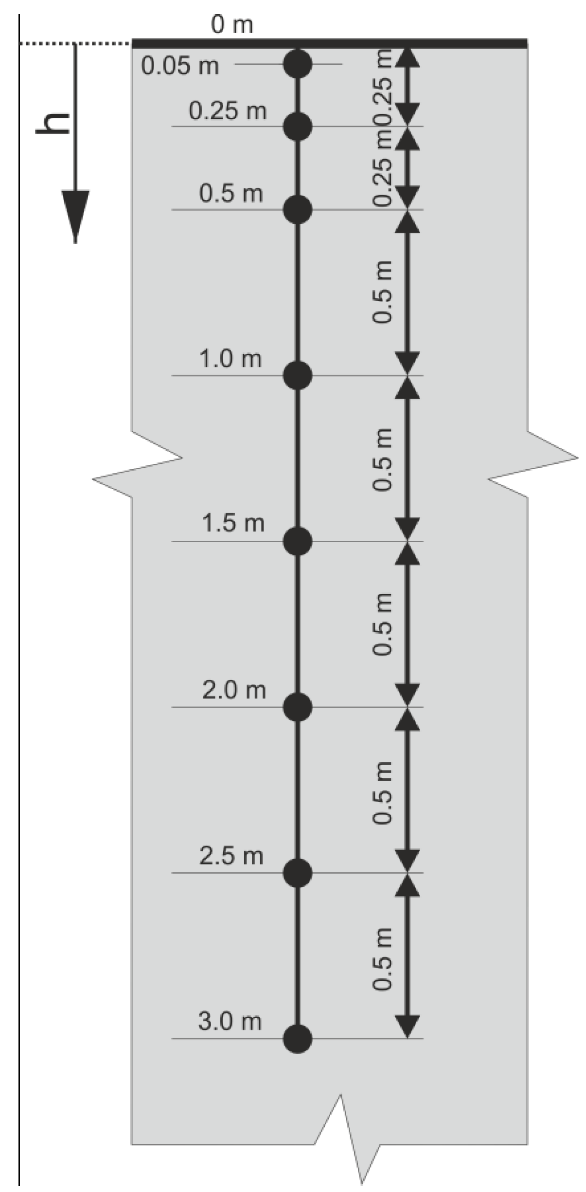
The temperature distribution tests were carried out in wells with a depth of 0.05–3 m. The location of the temperature sensors is shown in Figure 3. The first two temperature sensors were installed at depths of 0.05 and 0.25 m, while the next sensors were placed at intervals of 0.5 m. Allocation of sensors was completed densely, as recommended by Li et al. [32] and Al-Hinti et al. [33], opposite to several other previous studies, where the temperature was recorded every meter [34]. All sensors were installed in a layer of homogeneous soil. The temperature measurements were performed with DS18B20 sensors from Maxim Integrated Products, Inc., the characteristics and errors of which are in the manufacturer’s specification [35]. The maximum error of the DS18B20 sensor in the full measuring range is ±0.15 °C. Data recording took place at an interval of 1 h. The boreholes were made with a drill with a diameter of 30 mm; then, the sensors were installed on a thin polystyrene strip with a diameter of 4 mm, inserted into the hole and covered with native soil. The installation of the measuring probes was carried out in 2019, while the soil temperature measurements in the presented study were taken in the years 2020–2021.
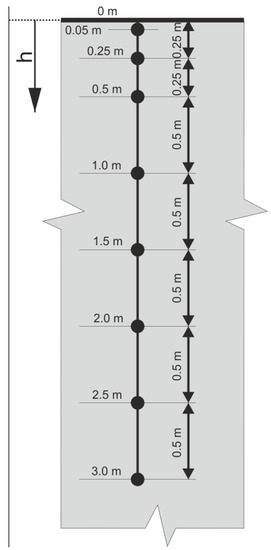
Figure 3.
Diagram of the test stand for measuring the temperature distribution in the soil.
Based on the PN-EN ISO 14688-1 standard [36], the soil in points 1 and 3 was classified as clay with a predominant grain size from 0.063 to 0.002 mm and up to 0.002 mm, while the soil in point 2 was classified as coarse sand with the predominant grain size from 0.63 to 2 mm.
The work also included the determination of the heat flux density according to the classical formula [37]:
where h is the coordinate of the soil depth (Figure 3), T is the ground temperature, and λ is the thermal conductivity coefficient of the soil.
The calculations were based on the thermal conductivity coefficients in accordance with PN-EN ISO 6946: 1999 [38] for point 1 (clay, wet conditions) 0.85 W/m/K, for point 2 (sand, wet conditions) 0.40 W/m/K, and for point 3 (clay, moderately humid conditions) 0.85 W/m/K.
The samples were placed in an oven at 60 °C for 48 h. Subsequently, they were ground and sieved through a 0.125 mm sieve. The resulting powder was analyzed by wavelength dispersive X-ray fluorescence spectrometry using the equipment PRIMUS IV, Rigaku, 4 kW power, and X-ray diffraction (XRD) using a Bruker D8 Discover A25 equipment with Cu-Kα radiation and goniometric scanning from 3 to 70 (2θ) at a speed of 0.01 °2θ s-1.
In order to carry out a proper identification of the mineralogy phases, the following procedure was performed according to [39] consisting of: (i) Saturation of the samples with K+ and (ii) and saturation with K+ and subsequent calcination at 550 °C. A sample from measurement point 1 was taken and saturated with a 1 N solution of ClK. The sample was allowed to stand for 2 h. After this time, the solution was centrifuged and the supernatant was removed. A total of 3 saturation steps were performed. Finally, the sample was washed with demineralized water, centrifuged, and placed in an oven at 60 °C for 48 h. Another part of the sample saturated with K+ was calcined at 550 °C for 2 h. At the end of each procedure, the dried samples were crushed with an agate stone and reanalyzed by XRD with a goniometric scan from 3 to 40 (2θ).
3. Results and Discussion
3.1. Analysis of Soil Samples
Table 2 shows the chemical composition results of the samples from measurement points 1, 2, and 3. SiO2 was the major oxide with percentages of 50.28%, 51.11%, and 48.36%, respectively. The Al2O3 (12.57%, 4.84%, and 12.11%), K2O (3.30%, 2.03%, and 2.24%), CaO (1.12%, 9.96%, and 2.65%), and Fe2O3 (4.69%, 1.16%, and 3.63%) contents also stood out. CO2 balance is related to the mass amount corresponding to the elements below the oxygen element in periodic table, and which was not included in the mentioned oxides.
Table 2.
Chemical composition of samples.
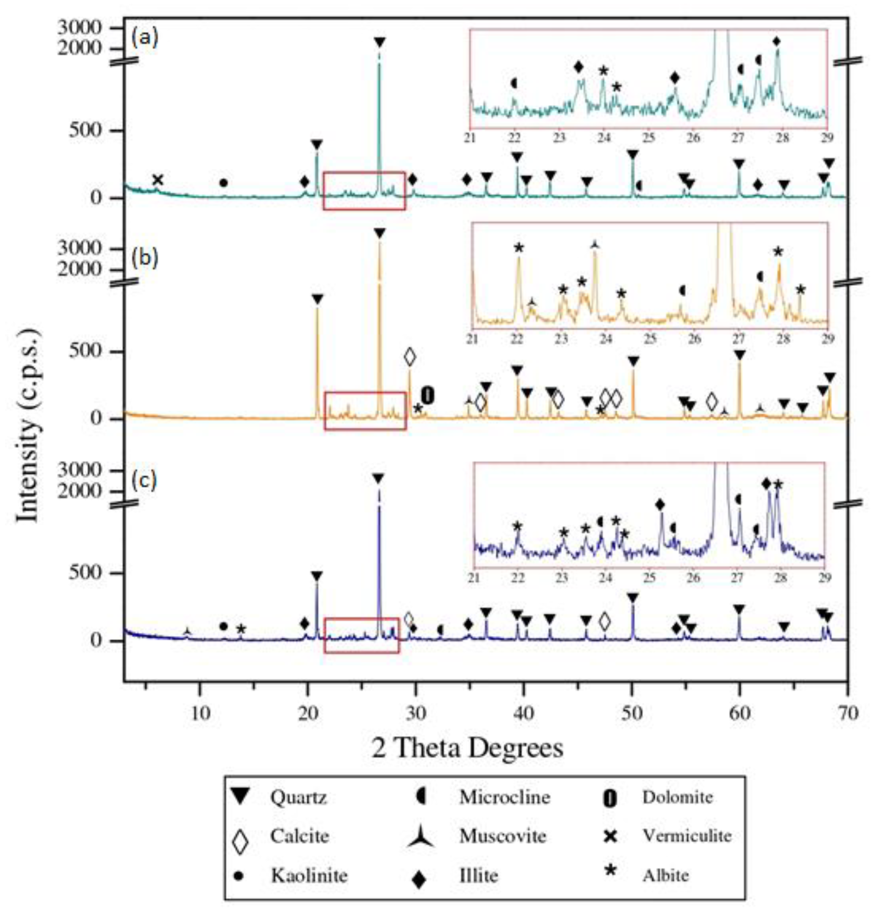
The XRD results of the samples from the different measurement points are shown in Figure 4. The main mineral phase found in the three samples corresponds to quartz (SiO2; 05-0490) (JCPD, 1995). The mineral phases microcline (KAlSi3O8; 19-0926) and albite (NaAlSi3O8; 09-0456) (JCPD, 1995) were also common in all three samples. Traces of illite (Al4KO12Si2; 02-0042) and kaolinite (Al2H4O9Si2; 14-0164) [40] were detected in samples from measurement points 1 and 3, as well as muscovite (Al3H2KO12Si3; 06-0263) [40] in samples from measurement points 2 and 3. The presence of calcite (CaCO3; 05-0586) [40] was also observed in samples from measurement points 2 and 3, being more representative in sample 2, according to Table 2. Finally, a trace of dolomite (CaMgO6; 11-0078) was recorded in the samples from measurement point 2.
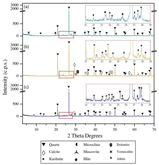
Figure 4.
Mineralogical analysis: (a) sample from measurement point 1; (b) sample from measurement point 2; (c) sample from measurement point 3.
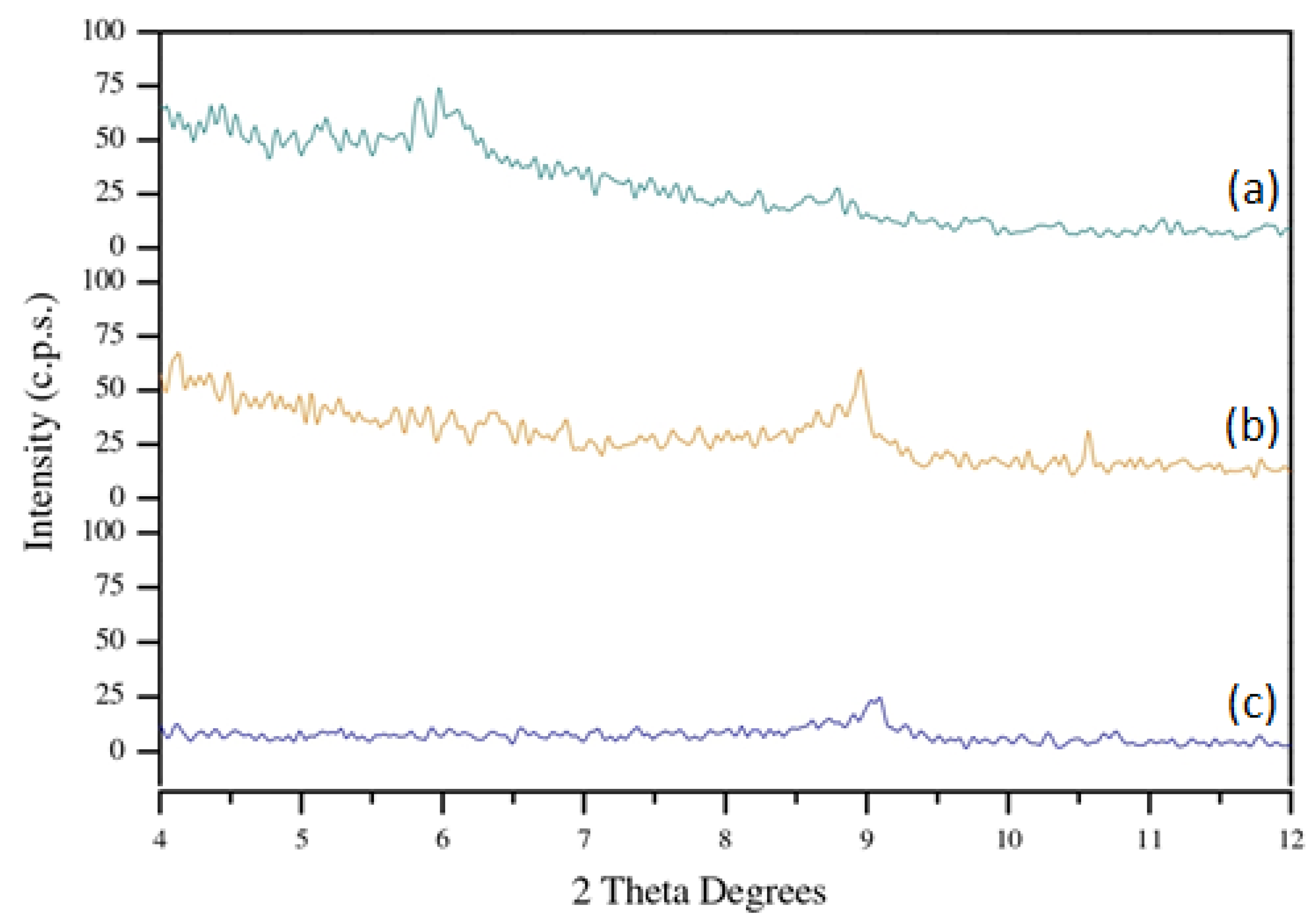
In Figure 4a, a reflection at 6.1 °2θ (d = 14.4 Å) was observed that could correspond to vermiculite (Si4O12Mg3H2; 16-0613) [40] or chlorite (Si2O9Mg3H4; 13-0003) [40]. In Figure 5a, a magnification (4–12 °2θ) of this XRD pattern is shown, as well as the patterns resulting from the treatment with a saturated solution in K+ (Figure 5b) and with a saturated solution in K+ solution and subsequently calcined at 550 °C (Figure 5c). A shift in the plane was shown that appears in Figure 5a towards 9 °2θ (d = 10 Å) (Figure 5b,c) that is in accordance with the presence of vermiculite (Si4O12Mg3H2; 16-0613) [40].
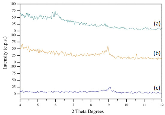
Figure 5.
Mineralogical identification: (a) sample from measurement point 1; (b) sample saturated in K+; (c) sample saturated in K+ and subsequently calcined at 550 °C.
These results show the similar composition of the samples measured in points No. 1 and 3 (clay soils), despite their different localization, and their differences with the sample of the point No. 2 (sand soil).
3.2. Soil Temperature Measurements
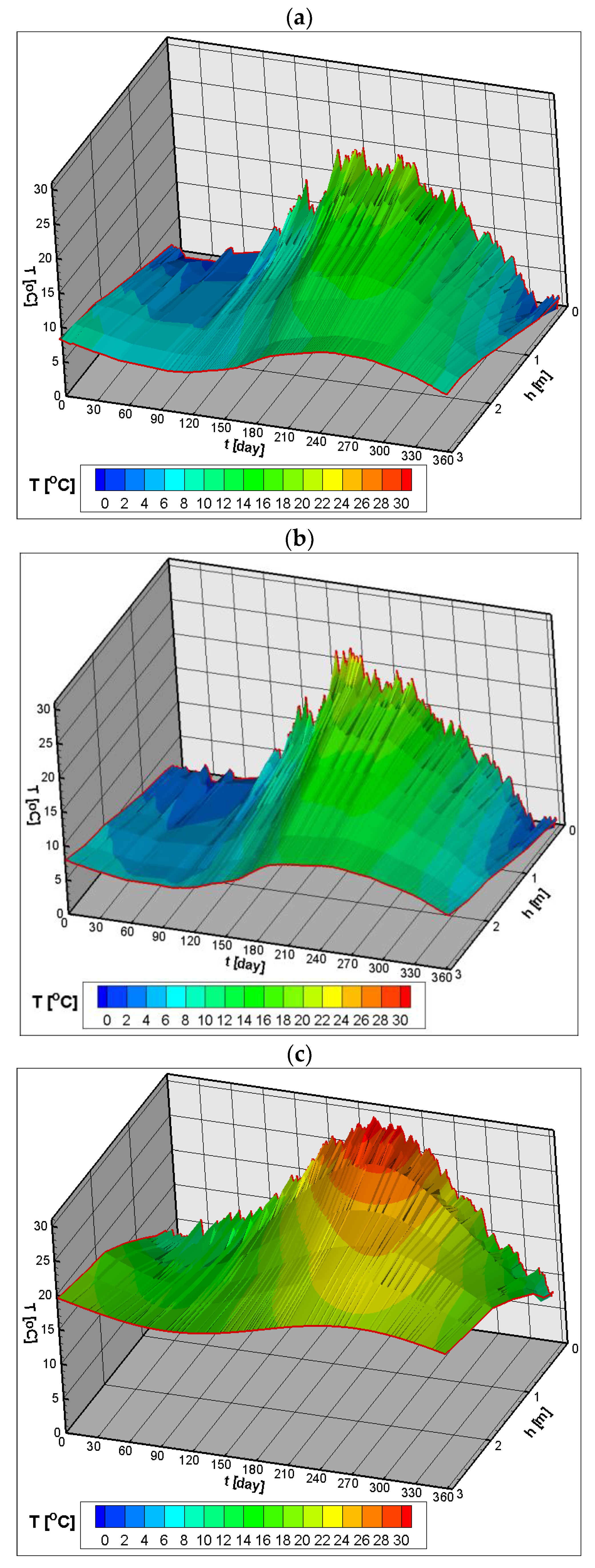
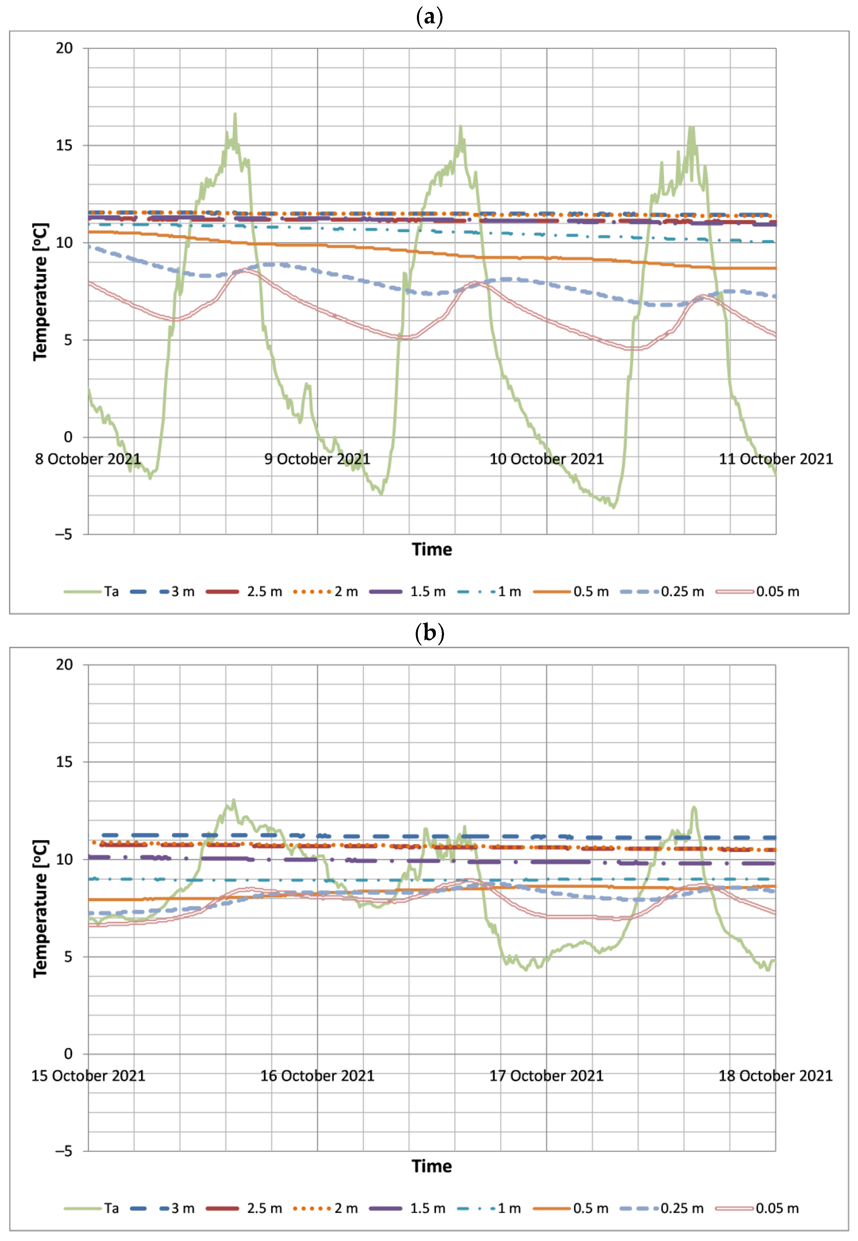
The results of the tests of temperature distribution in the soil as a function of depth for the range from 0.25 to 3 m and as a function of the number of days in a year for three measurement points are presented in Figure 6a–c. The results of the measurements show a significant influence of local increases and decreases in the outside temperature during the day on the individual layers of the soil, which is manifested by fluctuations in temperature values. Figure 7a shows an example of the impact of variable outside temperature, where the difference between the maximum and minimum outside temperature during the day is 20 °C, on the course of the ground temperature, while Figure 7b shows examples of temperature changes in the ground when the difference between the maximum and minimum outside temperature is equal to 8 °C. As the difference between the minimum and maximum outside air temperature increases, the temperature fluctuations in the ground increase. The effect of changes in external temperatures over one day on the ground temperature decreases with increasing borehole depth. The greatest temperature fluctuations occur at a depth of 0.25 cm.
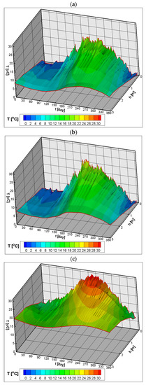
Figure 6.
Vertical distribution of temperature in the ground from 0.25 to 3 m as a function of the day of the year for the three measurement points: (a) No. 1, (b) No. 2, (c) No. 3.
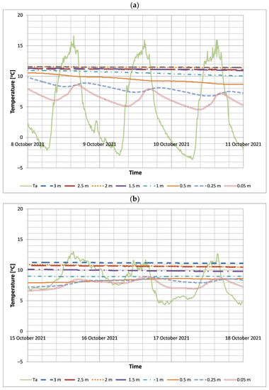
Figure 7.
The daily evolution of the temperatures in the ground of point No. 2 for the diurnal temperature ranges: (a) ΔTa = 20 °C, (b) ΔTa = 8 °C.
The average annual soil temperature for the h range from 0.25 to 3.00 m in the case of the measurement point No. 3 is 19.03 °C, while in the case of the measurement points No. 1 and No. 2, these temperatures are, respectively, 10.3 and 10 °C. In the case of measurement points No. 1 and No. 2, the values of annual average temperatures are similar despite the presence of different soil. In the case of measurement point No. 3, the annual average temperature values are about twice as high compared to points No. 1 and No. 2, which is caused by the location of the third measurement point in the subtropics. The annual average temperature values at the measurement point No. 3 are similar to the temperature values in the city of Huelva [41], which has the same climatic zone.
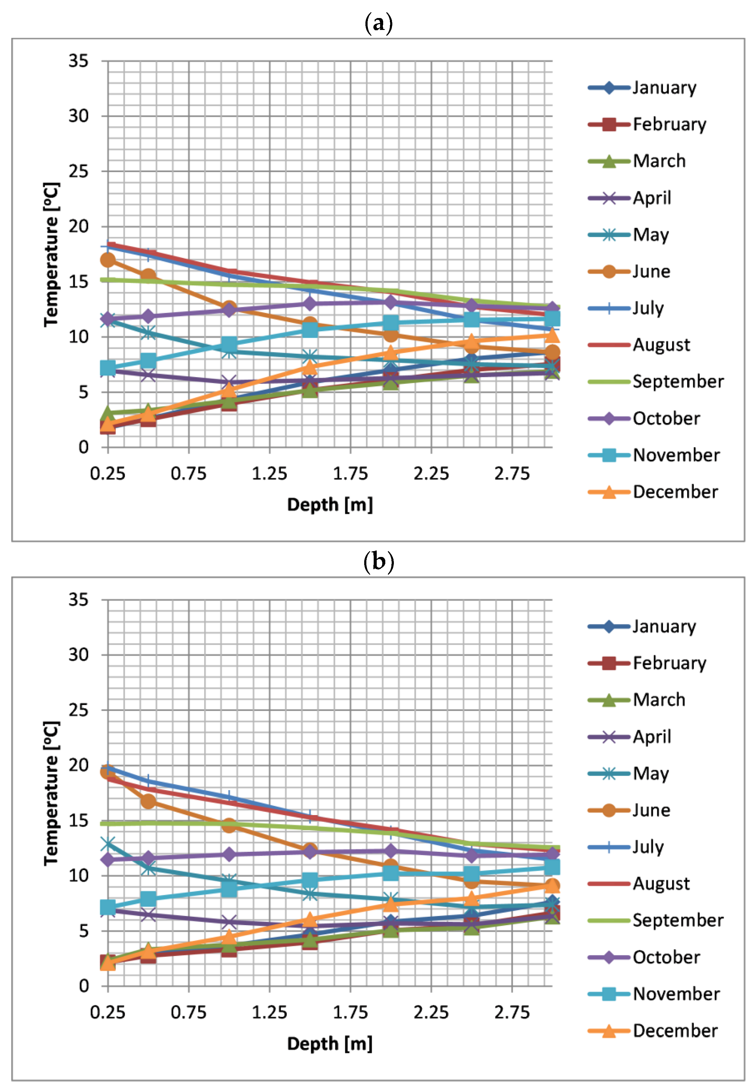
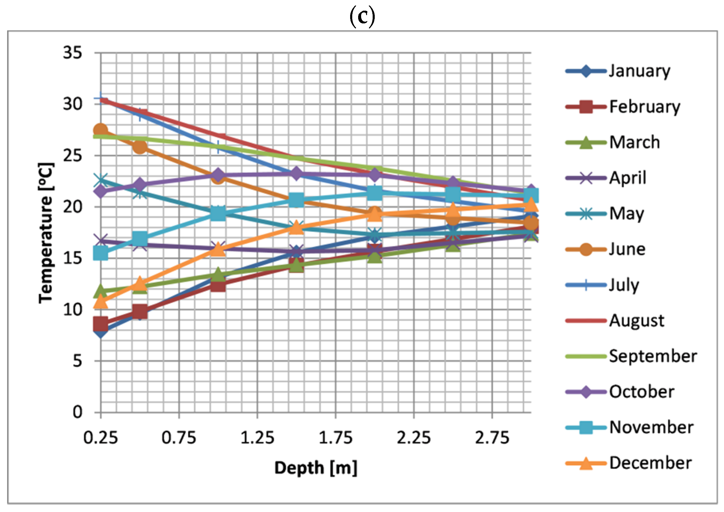
Figure 8a–c shows the average monthly temperatures for three measurement points as a function of depth. Comparing the monthly average temperature distributions for points No. 1 and No. 2, it can be noticed that the clay has higher temperature values in winter compared to sand, while in summer the opposite is true. In the case of measurement point No. 3 in Belmez, trends were similar to those obtained in the results of the research conducted in the city of Huelva [41], which, however, are characterized by higher temperature values.
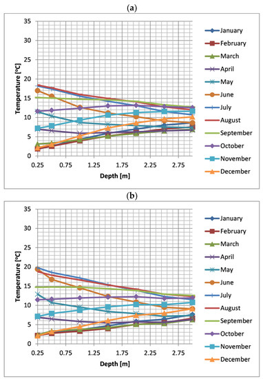
Figure 8.
Average monthly temperatures as a function of depth for three measurement points: (a) No. 1, (b) No. 2, (c) No. 3.
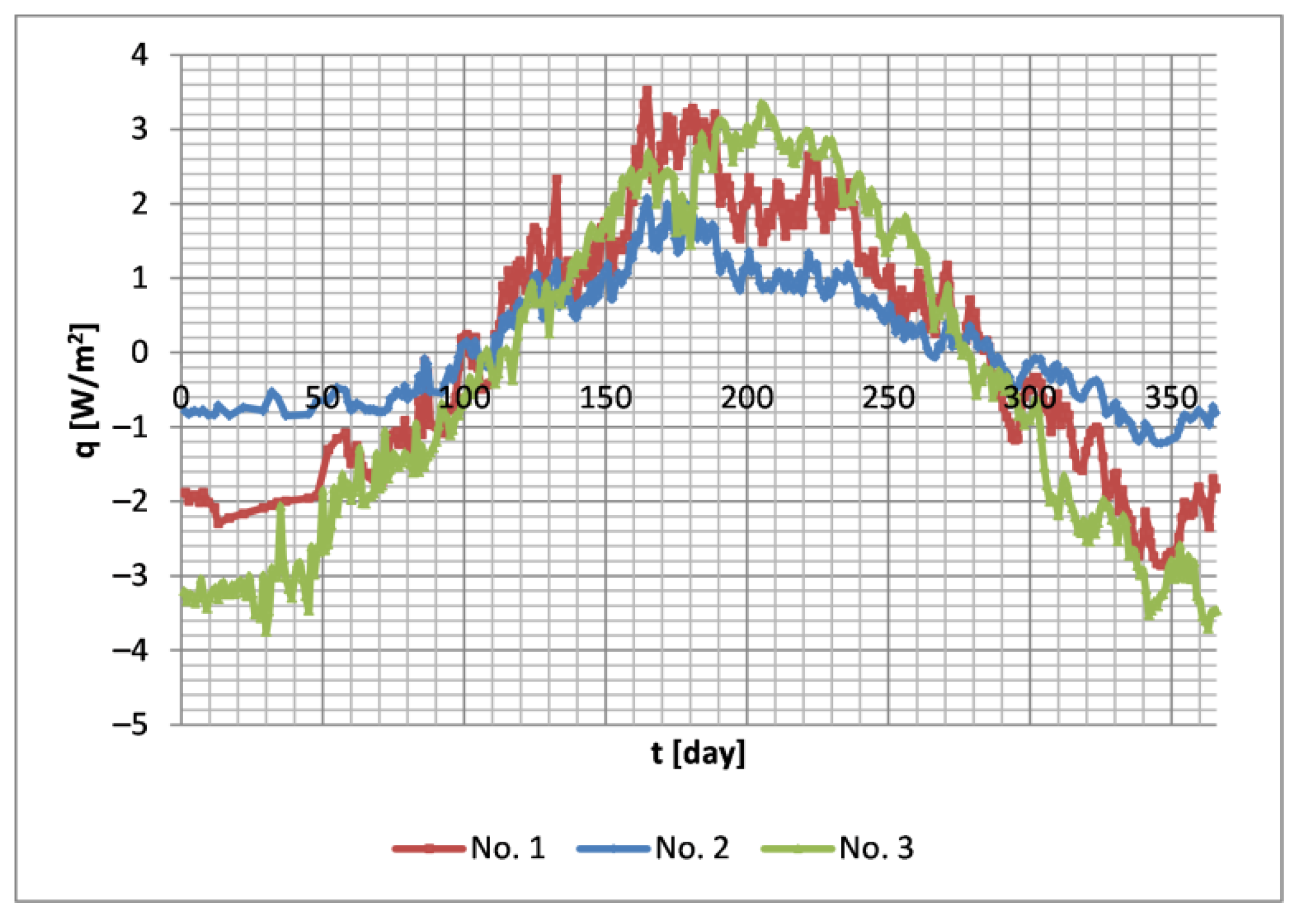
Figure 9 shows the heat flux densities in the layer from 0.25 to 3.00 m deep as a function of the number of days for measurement locations.
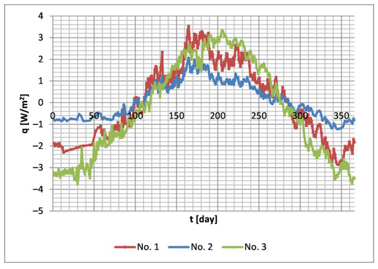
Figure 9.
Heat flux density in the ground layer 0.25–3.00 m as a function of the day of the year.
The heat flux density was determined according to the classical Formula (1):
where λ is the thermal conductivity coefficient of the soil, T0.25 is the temperature at a depth of 0.25 m, T3.00 is the temperature at a depth of 3 m, and Δh = 2.75 m is the soil layer for which heat conduction calculations were made.
In summer, the ground is heated both in a temperate climate (points No. 1 and No. 2) and in a subtropical climate (point No. 3), while in winter heat is transferred from the ground to the outside air. The highest heat flux values occur in the subtropical climate compared to the climate moderate, which is caused by greater direct solar radiation and higher outside temperatures in a subtropical climate [42]. When comparing the type of soil, it was noticed that the highest absolute values of heat flux density are conducted by clay (points No. 1 and No. 3), while the smallest are in the case of sand (point No. 2), which is due to the lower thermal conductivity coefficient for sand compared to clay.
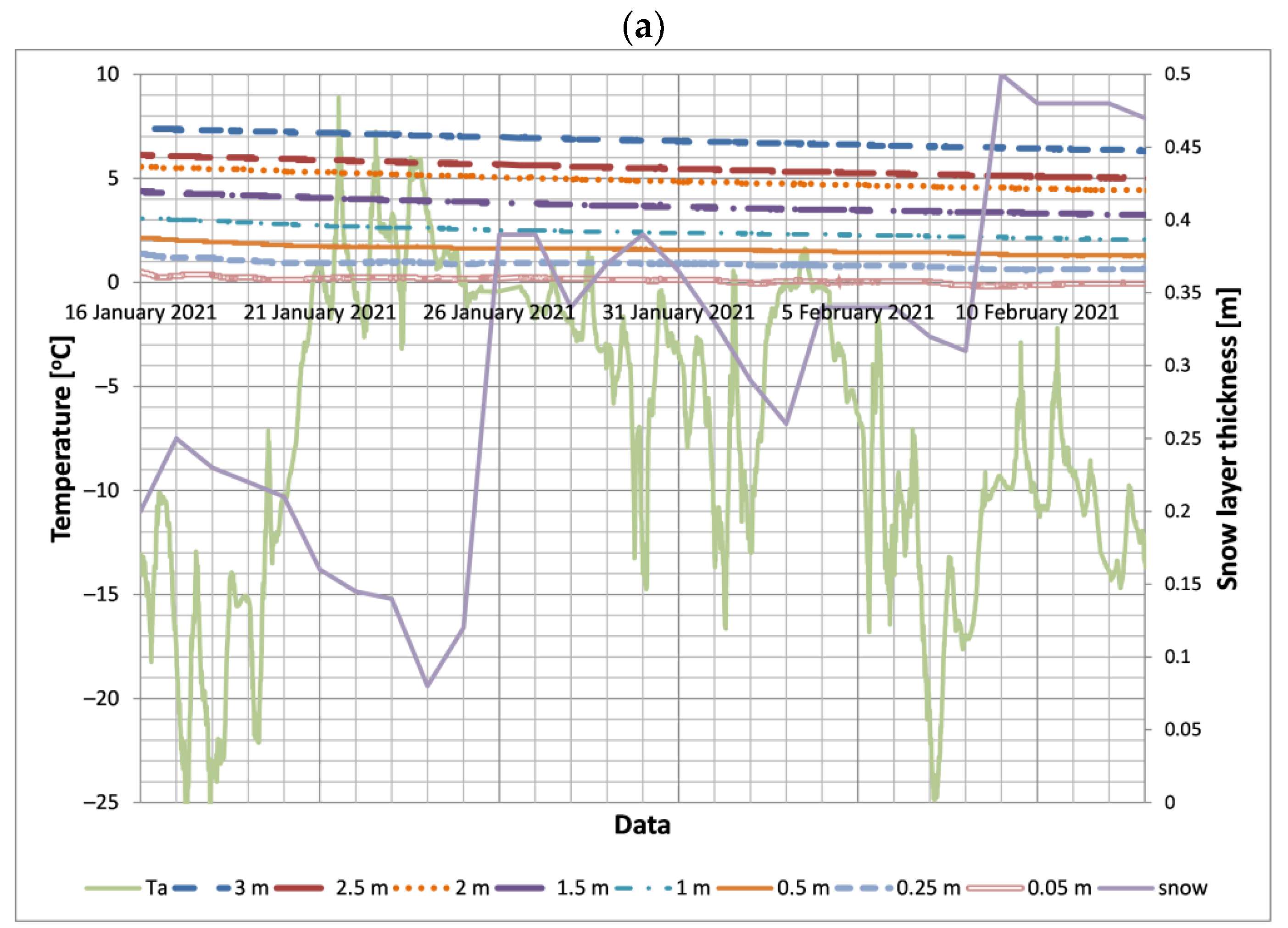
In winter, it can be noticed that in January and February the heat flux density graph in temperate climates is flattened, which is caused by the snow cover. Figure 10a,b shows changes in external and ground temperatures as well as the thickness of the snow layer in Bialystok (point No. 2) in January and February in 2021 and on several days in March 2021, respectively. In the period from 16 January 2021 to 13 February 2021 (Figure 10a, point No. 2), the average air temperature was −5.35 °C, the minimum air temperature was −25.38 °C, the average and minimum temperature at a depth of 0.05 m was 0.1 and −0.19 °C, respectively, while the average thickness of the snow layer was 0.31 m. In the snow-free period from 10 March 2021 to 12 March 2021(Figure 10a), the average air temperature was −2.81 °C, the minimum air temperature was −10.0 °C, the average and minimum temperature at a depth of 0.05 m was −0.68 and −1.44 °C, respectively. In the first period (from 16 January 2021 to 13 February 2021, Figure 10a), despite significantly lower air temperatures compared to the second period (from 10 March 2021 to 12 March 2021, Figure 10b), it can be noticed that the temperature in the 0.05 m layer is stabilized around zero and was higher compared to the second period in which the temperature in the 0.05 m layer oscillated around −0.6 °C. The stabilization of the ground temperature in the first period was influenced by the snow layer, which thermally insulated and protected the ground against freezing. The snow conductivity coefficient depends on the snow density and can range from 0.024 to 0.8 W/m/K [43,44].
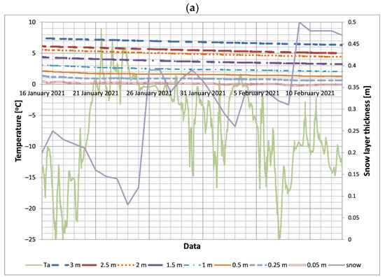
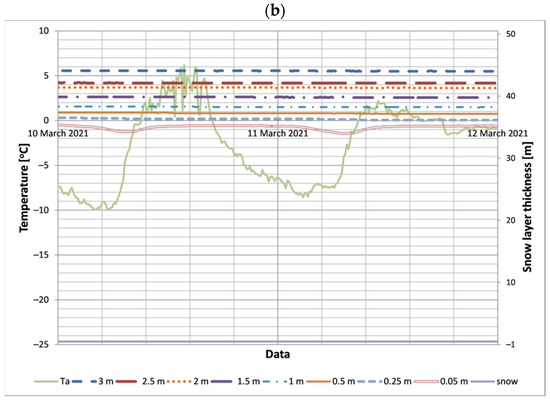
Figure 10.
Temperature changes in the ground of point No. 2 in the snowy (a) and snowless (b) winter period.
Heat conduction in the ground can be influenced by the composition of the soil. The second component present in the amount of clay is aluminum (III) oxide Al2O3 (Table 2), which is characterized by a significant value of the thermal conductivity coefficient from 12 to 38.5 W/m/K [45], which may significantly affect the heat flux. The percentage of Al2O3 in the sand (point 2) is about 2.5 times lower than that of clay (measurement points 2 and 3). The influence of individual elements in the soil on the heat flux is planned in the following tests.
3.3. A Simplified Model of the Temperature Distribution in the Ground
In order to develop a simplified model of soil temperature distribution as a function of depth and the number of the day during the year, an equation similar to the universal one of outside air temperature oscillation was considered [46]:
where A is the amplitude of temperature oscillation, B is the change of phase, and C is the horizontal translation. A dependence of this coefficient with the depth is assumed.
Modeling of meteorological parameters of the outside air by means of trigonometric functions is optionally performed in the commercial program WuFi [47,48]. The idea of proposed models based on the cyclical nature of the occurrence of temperatures in the ground results from the fact that the temperature in the ground changes daily at similar intervals close to the meteorological time series [49]. Equation (2) is most often used in many scientific papers and computational programs for simplified simulation of the outside air temperature during the year. The use of the cosine function in the equation for simulating temperatures is related to the occurrence of seasons that are a consequence of the Earth’s orbital movement around the Sun and the inclination of the Earth’s axis to the orbit plane of this movement, which translates into changes in the outside air temperature. Due to the large temperature fluctuations in the soil layer of 0.05 m, resulting from the significant influence of air temperature and solar radiation on this layer, a soil layer from 0.25 to 3.0 m was selected for the model development.
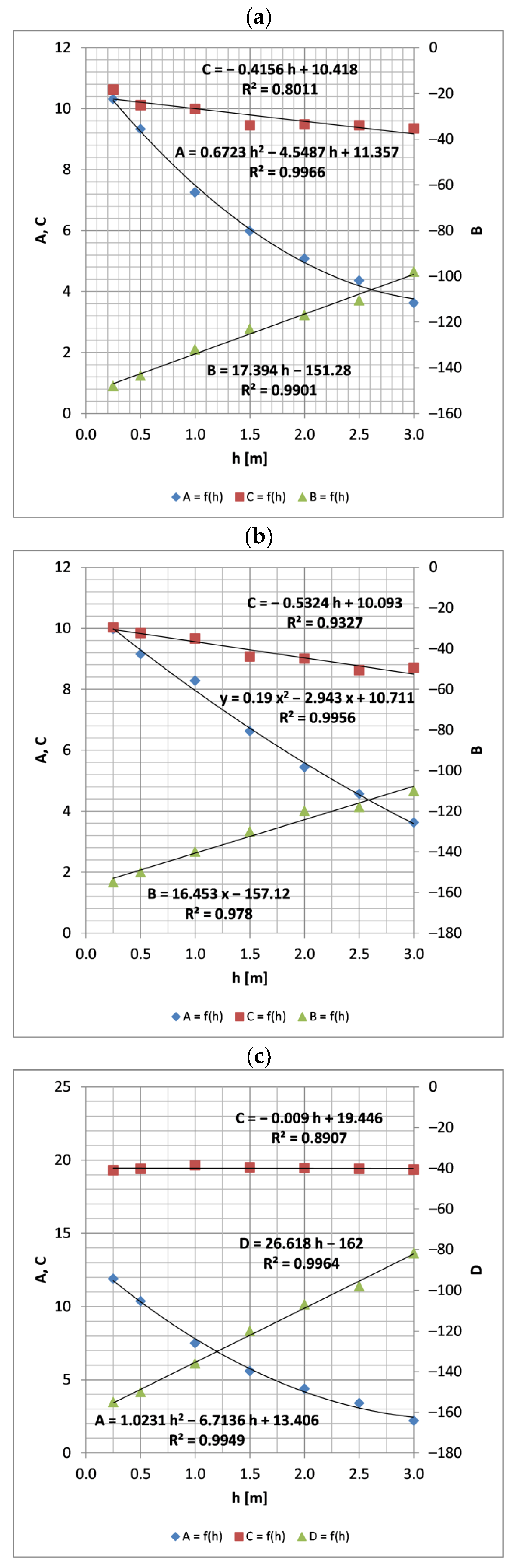
Based on the data obtained from the experiment for selected measurement points in three locations, the coefficients A, B, and C were determined, which are presented in Figure 11a-c for measurement points 1, 2, and 3, respectively. The B and C coefficients have a linear dependence on the depth coordinate h, while a quadratic dependence is observed for the A coefficient.
Figure 11.
Dependence of A, B, and C coefficients on the depth h for three measurement points: (a) No. 1, (b) No. 2, (c) No. 3.
Then the experimental data can be fitted to following function:
The values of the obtained fitting coefficients are shown in Table 3.
Table 3.
Fitting coefficients of Equations (4)-(6) and their physical meaning.
The values of these coefficients are related with the thermal properties of the soils. To see this fact, we can compare the temperature distribution of Equation (3) with the solution of the heat conduction equation:
where ρ is the density, C is the heat capacity, and k the thermal conductivity of the soil, considering the ground as a homogenous semi-infinite layer and the boundary condition in z = 0 equal to the soil surface temperature. This solution is given by [41]:
with Tm = the average temperature of the soil surface, A0 = the amplitude of the temperature oscillation, t0 = the time shift, and α = the thermal diffusivity of the soil, that is equal to:
For shallow positions (h < 2.5 m), the exponential term can be approximated (Taylor series) by:
and the temperature distribution of the Equation (7) by:
Comparing the Equations (3) and (8) for the temperature distribution, the physical meanings of the coefficients of Equations (4)–(6) can be obtained (see Table 3).
Using the relationships of Table 3, the values of thermal diffusivity and other parameters of Equation (11) can be obtained from the experimental measures. The experimental values of these parameters for the three measurement points are presented in Table 4. In this table, the thermal diffusivity α(A) and α(B) are the diffusivity values obtained from the amplitude and phase variations, respectively (from a and b coefficients, respectively).
Table 4.
Values of the thermal diffusivities α(A) and α(B), and other parameters of Equation (10) for measurement points No. 1, No. 2, and No. 3.
The obtained values of the average temperature of the soil surface, Tm, agree with the measured values 10.3, 10, and 19.03 °C, presented in Section 3.2. It must be noted that the C coefficient of Equation (6) should have to be theoretically constant and equal to this temperature in the homogenous semi-infinite approximation. However, Figure 11 shows that it only happened for the point No. 3 in Belmez. In the case of points No. 1 and 2, the C coefficients decrease with the depth h. It can be explained by the soil humidity in these points, that causes the homogeneity condition to not be fully fitted. The different soil humidity causes the heat capacity, the thermal conductivity, and the thermal diffusivity to vary from a depth position to another one. This effect is not happening in the dry soil of the point No. 3.
Regarding the amplitude of the temperature oscillation Ao, the maximum value corresponds to Belmez localization, by the higher values of outdoor temperature in this point.
The differences between the thermal diffusivities calculated from amplitude and phase variations could be due to different reasons. Kusuda and Achenbach [50] proposed errors of the fitting by inconsistent temperature depth data or errors of the phase determination by temporal fluctuation. In our case, highest differences correspond to the points No. 1 and 2. So, the differences could also result from the inhomogeneities of the wet soils. The results presented in Table 4 show that the lowest value of the thermal diffusivity is for the Belmez with 0.5 × 10⁻⁶ m2/s, which is typical of a dry clay (see Table 1 in [41]). The point No. 1, with a similar type of soil, presents a higher thermal diffusivity about 0.73 × 10⁻⁶ m2/s by the humidity of this localization. The highest value of this diffusivity is for point No. 2 with a value typical of wet sand.
Based on the experimental results [51,52], the relationship between thermal diffusivity and the moisture content in the clay can be seen, that thermal diffusivity increases with increasing soil moisture content. Estimated values of α (A) and α (B) indicate higher moisture content in measurement point 1 compared to measurement point 3, which is caused by higher outside temperatures and much greater direct solar radiation at measurement point 3. It should be noted here that a thorough examination of the moisture content in the soil requires thorough laboratory tests.
The relative error of the model (3) was determined as the temperature difference of the Texp experiment and the solution of the temperature of the simplified Tnum model (3) related to the temperature from the experiment:
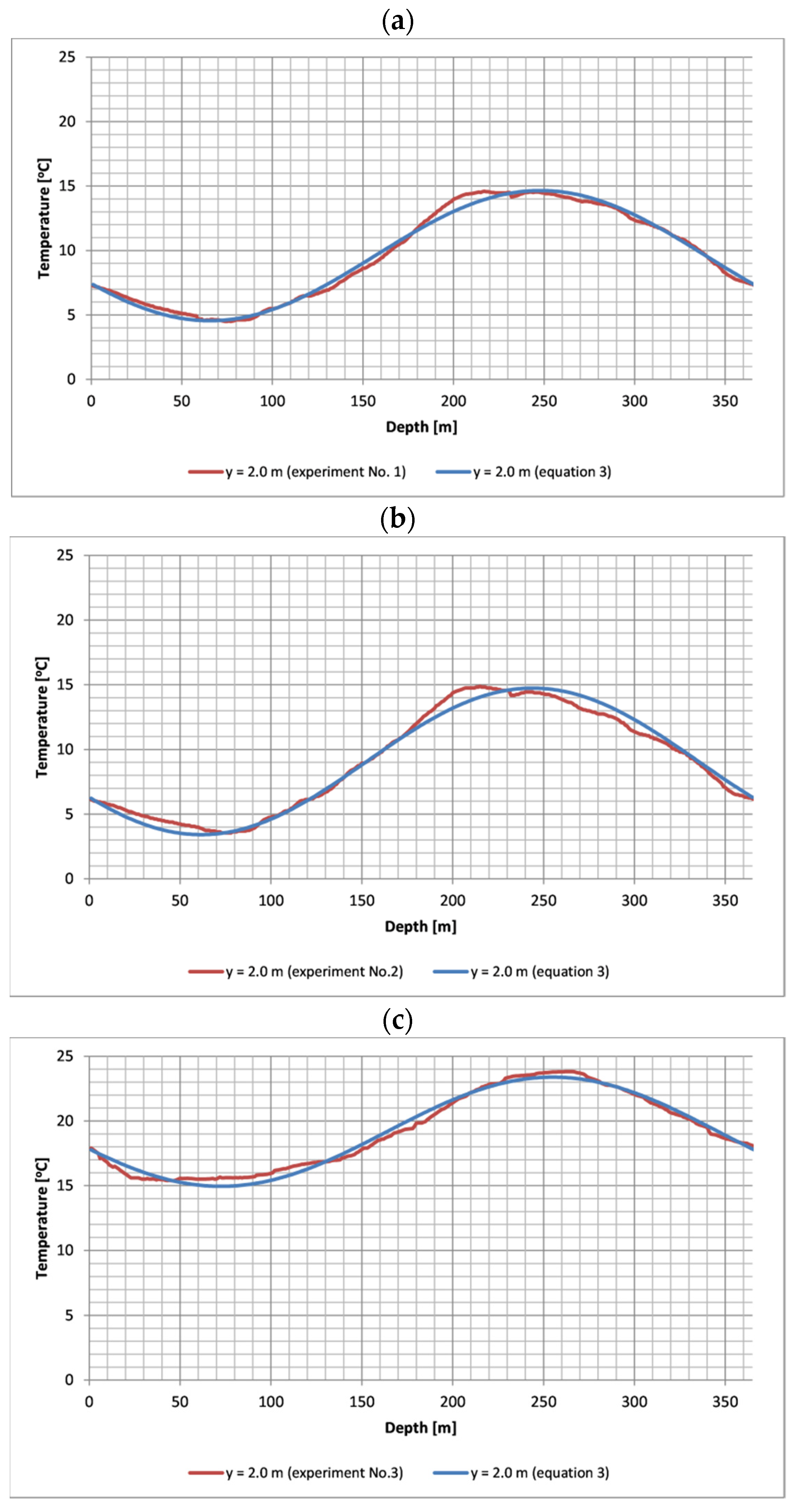
The average relative error from individual measurement series, determined according to formula (12) for all depths in accordance with Figure 2, did not exceed 7.7%, 5.76%, and 2.9%, respectively, for measurement locations 1, 2, and 3. The comparison of the model with the experiment is shown in Figure 12a–c at a depth of 2 m, respectively, for measurement points 1, 2, and 3. The presented model works well both in the temperate and subtropical climate zones.
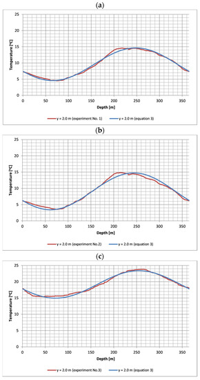
Figure 12.
Comparison of the temperature values from the experiments and the computational model at h = 2 m for three measurement points: (a) No. 1, (b) No. 2, (c) No. 3.
After substituting the Formula (3) to (1), the following form of heat flux density in the ground layer from 0.25 to 3.0 m was obtained:
where the coefficients are presented in Equations (4)–(6) and Table 3.
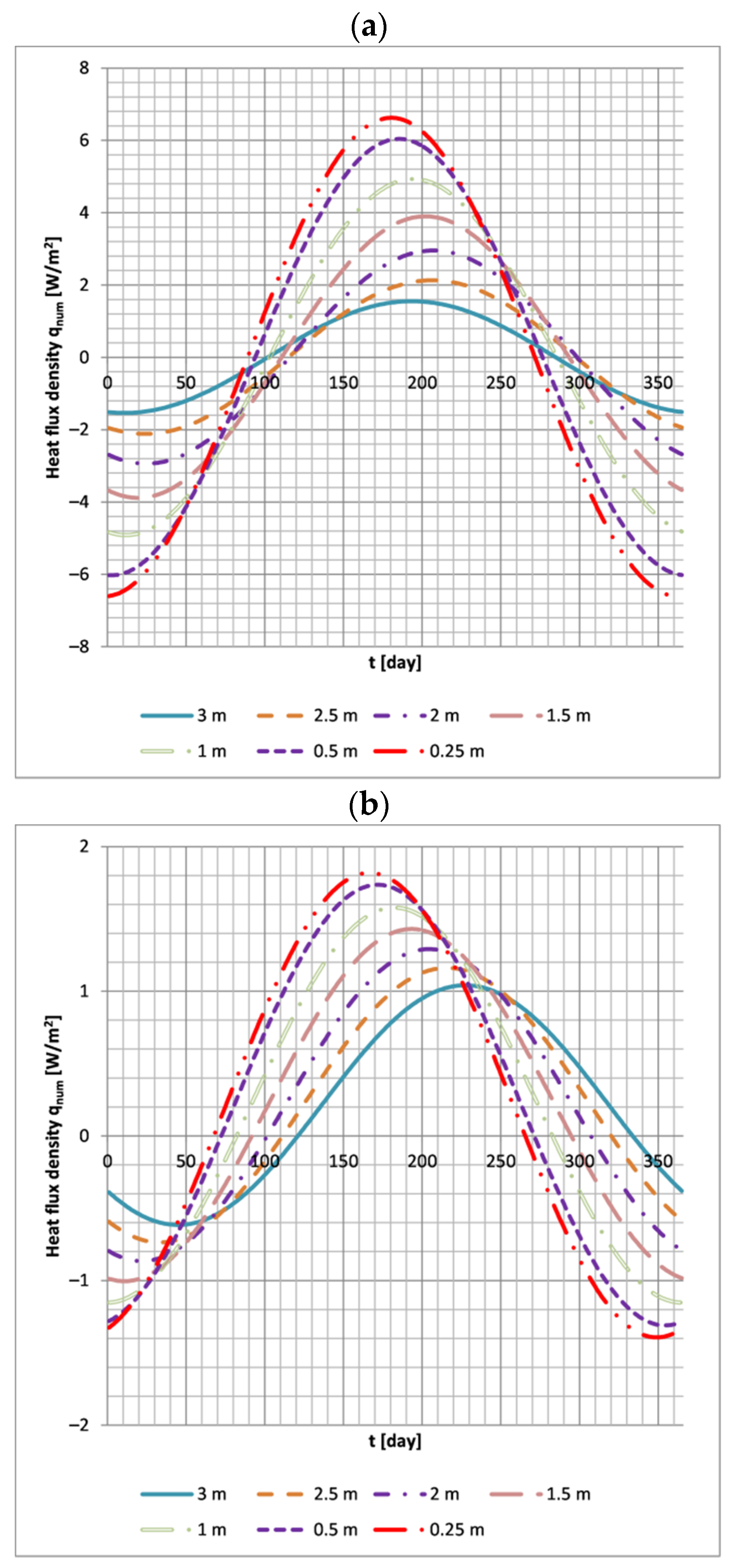
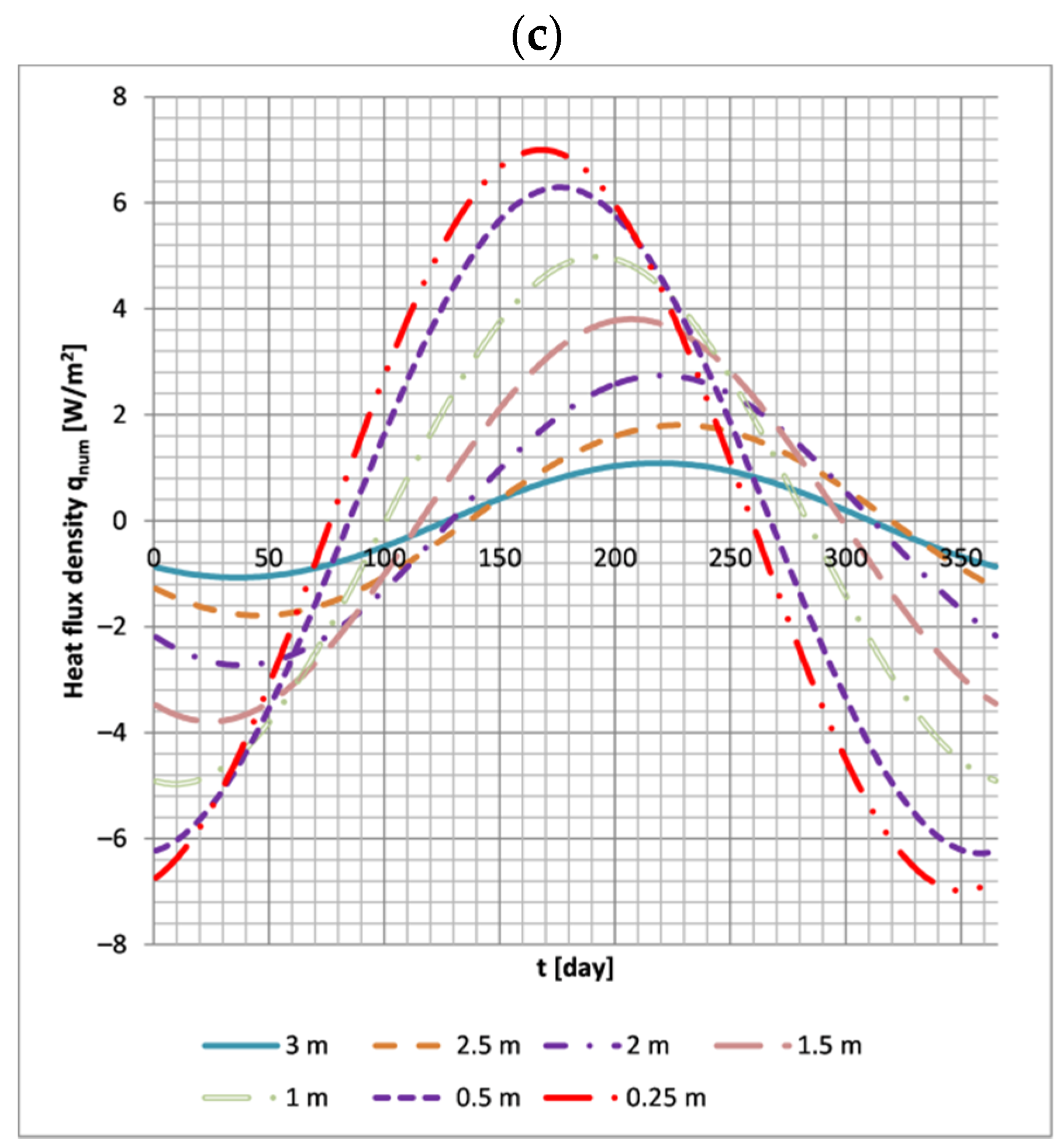
Figure 13a–c shows the results of the heat flux density calculations from formula (9) for a depth of 0.25 m < h < 3.0 m for measurement locations 1, 2, and 3, respectively. The greatest amplitudes of heat flux density changes as a function of days are found in shallower soil layers, which is related to the greater influence of air temperature and solar radiation on heat exchange in the ground. The significant influence of solar radiation on soil temperature was presented in [24]. The values of the heat flux density amplitudes decrease with the soil depth. In subtropics (measurement point number 3), the heat flux densities are higher compared to measurement points located in temperate climates (measurement point numbers 1 and 2). The work [42] indicates that the annual GHI (Global Horizontal Irradiation) value in the city of Cordoba, which is located near measurement point 3 (Belmez), was 1972 kWh/m2/year, while in the case of Białystok (measurement point numbers 1 and 2) the annual GHI value is 1086 kWh/m2/year. The lowest values of heat flux density occur at measurement point No. 2, which is related to the low thermal conductivity coefficient of sand (No. 1) compared to clay (No. 1 and 3). Based on the analysis of the graphs, it can be noticed that at a depth of 3 m, the heat flux density trends are similar for three points. With decreasing depth, the fluctuations in the heat flux density are greater.
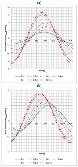
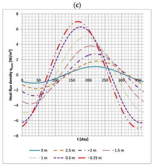
Figure 13.
Heat flux density in the ground layer 0.25–3.00 m determined from Equation (9) as a function of the number of days for the three measurement points: (a) No. 1, (b) No. 2, (c) No. 3.
4. Conclusions
The paper presented the results of research on the temperature distribution in homogeneous soil at a depth of 0.25–3 m. The research was carried out for two wells in a selected location in a temperate climate and one well located in a selected point in a subtropical climate. The choice of the location of the measurement points was related to the type that most often occurs in a given area. The tests were carried out for clay (temperate and subtropical climate) and for sand (temperate climate).
Among the studied location points, the highest values of soil temperatures up to 3.0 m deep are found in the subtropical climate (location No. 3 Belmez), which is related to the highest GHI value in this region. The amplitudes of the heat flux density values transferred in the layer at the depth from 0.25 to 3.00 m in clay are greater than in sand, which is related to the higher thermal conductivity of clay compared to sand.
Based on the research, a model of temperature distribution as a function of depth and the number of days in a year was developed. The developed model can be used as a boundary condition in the design of heating networks and heat exchangers. The presented simplified model can also be developed in other locations and soils, and it is possible to create a database of temperature distributions in different regions of the world. In subsequent studies, tests for other types of soil are planned.
Author Contributions
Conceptualization, T.J.T., D.A.K. and A.R.; methodology, T.J.T., D.A.K. and A.R.; investigation, T.J.T., D.A.K., A.R., J.M.F.-R. and A.L.-L.; writing—original draft preparation, T.J.T., D.A.K., A.R., J.M.F.-R. and A.L.-L.; supervision, D.A.K.; project administration, D.A.K.; funding acquisition, D.A.K. All authors have read and agreed to the published version of the manuscript.
Funding
This scientific project was financed from funds of BUT InterAcademic Partnerships (PPI/APM/2018/1/00033/DEC/1) NAWA project and WZ/WB-IIŚ/ 7/2022. The research was carried out as part of the Białystok University of Technology grant and financed from a research subsidy provided by the minister responsible for science. The study was conducted in the Scientific Cooperation Agreement, “The possibility of the renewable energy sources usage in the context of improving energy efficiency and air quality in the buildings and civil constructions” between BUT and UCO.
Institutional Review Board Statement
Not applicable.
Informed Consent Statement
Not applicable.
Data Availability Statement
Not applicable.
Conflicts of Interest
The authors declare no conflict of interest.
References
- Sliwa, T.; Sojczyńska, A.; Rosen, A.M.; Kowalski, T. Evaluation of Temperature Profiling Quality in Determining Energy Efficiencies of Borehole Heat Exchangers. Geothermics 2019, 78, 129–137. [Google Scholar] [CrossRef]
- Sakata, Y.; Katsura, T.; Serageldin, A.A.; Nagano, K.; Ooe, M. Evaluating Variability of Ground Thermal Conductivity within a Steep Site by History Matching Underground Distributed Temperatures from Thermal Response Tests. Energies 2021, 14, 1872. [Google Scholar] [CrossRef]
- Sliwa, T.; Sapińska-Śliwa, A.; Gonet, A.; Kowalski, T.; Sojczyńska, A. Geothermal Boreholes in Poland—Overview of the Current State of Knowledge. Energies 2021, 14, 3251. [Google Scholar] [CrossRef]
- Katsura, T.; Sakata, Y.; Ding, L.; Nagano, K. Development of Simulation Tool for Ground Source Heat Pump Systems Influenced by Ground Surface. Energies 2020, 13, 4491. [Google Scholar] [CrossRef]
- Mitchell, M.S.; Spitler, J.D. An Enhanced Vertical Ground Heat Exchanger Model for Whole-Building Energy Simulation. Energies 2020, 13, 4058. [Google Scholar] [CrossRef]
- Gao, S.; Tang, C.; Luo, W.; Han, J.; Teng, B. A New Analytical Model for Calculating Transient Temperature Response of Vertical Ground Heat Exchangers with a Single U-Shaped Tube. Energies 2020, 13, 2120. [Google Scholar] [CrossRef]
- Shimada, Y.; Uchida, Y.; Takashima, I.; Chotpantarat, S.; Widiatmojo, A.; Chokchai, S.; Charusiri, P.; Kurishima, H.; Tokimatsu, K. A Study on the Operational Condition of a Ground Source Heat Pump in Bangkok Based on a Field Experiment and Simulation. Energies 2020, 13, 274. [Google Scholar] [CrossRef] [Green Version]
- Leski, K.; Luty, P.; Gwadera, M.; Larwa, B. Numerical Analysis of Minimum Ground Temperature for Heat Extraction in Horizontal Ground Heat Exchangers. Energies 2021, 14, 5487. [Google Scholar] [CrossRef]
- Gwadera, M.; Kupiec, K. Modeling the Temperature Field in the Ground with an Installed Slinky-Coil Heat Exchanger. Energies 2021, 14, 4010. [Google Scholar] [CrossRef]
- Zhou, Y.; Bidarmaghz, A.; Makasis, N.; Narsilio, G. Ground-Source Heat Pump Systems: The Effects of Variable Trench Separations and Pipe Configurations in Horizontal Ground Heat Exchangers. Energies 2021, 14, 3919. [Google Scholar] [CrossRef]
- Kim, K.; Kim, J.; Nam, Y.; Lee, E.; Kang, E.; Entchev, E. Analysis of Heat Exchange Rate for Low-Depth Modular Ground Heat Exchanger through Real-Scale Experiment. Energies 2021, 14, 1893. [Google Scholar] [CrossRef]
- Sorokins, J.; Borodinecs, A.; Zemitis, J. Application of ground-to-air heat exchanger for preheating of supply air. IOP Conf. Ser. Earth Environ. Sci. 2017, 90, 012002. [Google Scholar] [CrossRef] [Green Version]
- EN 15698-1:2020-01; District Heating Pipes—Bonded Twin Pipe Systems for Directly Buried Hot Water Networks—Part 1: Factory Made Twin Pipe Assembly of Steel Service Pipes, Polyurethane Thermal Insulation and One Casing of Polyethylene. European Committee for Standardization: Brussels, Belgium, 2019.
- EN 13941-1:2019; District Heating Pipes—Design and Installation of Thermal Insulated Bonded Single and Twin Pipe Systems for Directly Buried Hot Water Networks—Part 1: Design. European Committee for Standardization: Brussels, Belgium, 2019.
- Bøhm, B.; Kristjansson, H. Single, twin and triple buried heating pipes: On potential savings in heat losses and costs. Int. J. Energy Res. 2005, 29, 1301–1312. [Google Scholar] [CrossRef]
- Van der Heijde, B.; Aertgeerts, A.; Helsen, L. Modelling steady-state thermal behavior of double thermal network pipes. Int. J. Therm. Sci. 2017, 117, 316–327. [Google Scholar] [CrossRef] [Green Version]
- Krawczyk, D.A.; Teleszewski, T.J. Optimization of Geometric Parameters of Thermal Insulation of Pre-Insulated Double Pipes. Energies 2019, 12, 1012. [Google Scholar] [CrossRef] [Green Version]
- Danielewicz, J.; Śniechowska, B.; Sayegh, M.A.; Fidorów, N.; Jouhara, H. Three-dimensional numerical model of heat losses from district heating network pre-insulated pipes buried in the ground. Energy 2016, 108, 172–184. [Google Scholar] [CrossRef] [Green Version]
- Danielewicz, J.; Fidorow, N.; Jadwiszczak, P.; Szulgowska-Zgrzywa, M. The exploitation costs for various heating systems according to the energetic certification law in Poland. Energy Sources Part B Econ. Plan. Policy 2014, 9, 301–306. [Google Scholar] [CrossRef]
- Information Materials of Logstor Companies. 2012. (01/02). Available online: http://www.logstor.com/ (accessed on 1 March 2022).
- Terradas-III, G.; Triolo, J.M.; Pham, C.H.; Martí-Herrero, J.; Sommer, S.G. Thermic model to predict biogas production in unheated fixed dome digesters buried in the ground. Environ. Sci. Technol. 2014, 48, 3253–3262. [Google Scholar] [CrossRef]
- Rainier, H.; Nouceiba, A.; Yves, J.; Marie-Noëlle, P. Modeling and simulation of heat transfer phenomena in a semi-buried anaerobic digester. Chem. Eng. Res. Des. 2017, 119, 101–116. [Google Scholar]
- Teleszewski, T.J.; Żukowski, M. Analysis of Heat Loss of a Biogas Anaerobic Digester in Weather Conditions in Poland. J. Ecol. Eng. 2018, 19, 242–250. [Google Scholar] [CrossRef]
- Larwa, B. Heat Transfer Model to Predict Temperature Distribution in the Ground. Energies 2019, 12, 25. [Google Scholar] [CrossRef] [Green Version]
- Kupiec, K.; Larwa, B.; Gwadera, M. Heat transfer in horizontal ground heat exchangers. Appl. Therm. Eng. 2015, 75, 270–276. [Google Scholar] [CrossRef]
- Ouzzane, M.; Eslami-Nejad, P.; Aidoun, Z.; Lamarche, L. Analysis of the convective heat exchange effect on the undisturbed ground temperature. Sol. Energy 2014, 108, 340–347. [Google Scholar] [CrossRef]
- Gwadera, M.; Larwa, B.; Kupiec, K. Undisturbed ground temperature—Different methods of determination. Sustainability 2017, 9, 2055. [Google Scholar] [CrossRef] [Green Version]
- Carslaw, H.S.; Jaeger, J.C. Conduction of Heat in Solids, 2nd ed.; Clarendon Press: Oxford, UK, 1959; ISBN 978-0198533030. [Google Scholar]
- Rao, K.G. Estimation of the exchange coefficient of heat during low wind convective conditions. Bound. Layer Meteorol. 2004, 111, 247–273. [Google Scholar] [CrossRef]
- McAdams, W.H. Heat Transmission; McGraw-Hill: New York, NY, USA, 1954. [Google Scholar]
- Molina-Rodea, R.; Wong-Loya, J.A. A new model to predict subsoil-thermal profiles based on seasonal rain conditions and soil properties. Geothermics 2021, 97, 102261. [Google Scholar] [CrossRef]
- Le, A.T.; Wang, L.; Wang, Y.; Li, D. Measurement investigation on the feasibility of shallow geothermal energy for heating and cooling applied in agricultural greenhouses of Shouguang City: Ground temperature profiles and geothermal potential. Inf. Processing Agric. 2021, 8, 251–269. [Google Scholar] [CrossRef]
- Al-Hinti, I.; Al-Muhtady, A.; Al-Kouz, W. Measurement and modelling of the ground temperature profile in Zarqa, Jordan for geothermal heat pump applications. Appl. Therm. Eng. 2017, 123, 131–137. [Google Scholar] [CrossRef]
- Tong, C.; Li, X.; Duanmu, L.; Wang, H. Prediction of the temperature profiles for shallow ground in cold region and cold winter hot summer region of China. Energy Build. 2021, 242, 110946. [Google Scholar] [CrossRef]
- Available online: https://datasheets.maximintegrated.com/en/ds/DS18B20.pdf (accessed on 23 April 2022).
- PN-EN ISO 14688-1:2018-05; Geotechnical Investigation and Testing—Identification and Classification of Soil—Part 1: Identification and Description (ISO 14688-1:2017). European Committee for Standardization: Brussels, Belgium, 2017.
- Rose, C.W. Agricultural Physics; Pergamon: Oxford, UK, 1966; p. 230. [Google Scholar]
- PN-EN ISO 6946: 1999; Building Components and Building Elements—Thermal Resistance and Thermal Transmittance—Calculation Method. European Committee for Standardization: Brussels, Belgium, 1996.
- Whittig, L.D.; Allardice, W.R. X-ray diffraction techniques. In Methods of Soil Analysis. Part 1. Physical and Mineralogical Methods, 2nd ed.; Klute, A., Ed.; Agron. Monogr. 9; ASA and SSSA: Madison, WI, USA, 1986; pp. 331–362. [Google Scholar]
- JCPD. Joint Committee on Powder Diffraction Standards; International Center for Diffraction Data: Swarthmore, PA, USA, 1995. [Google Scholar]
- Andújar Márquez, J.M.; Martínez Bohórquez, M.Á.; Gómez Melgar, S. Ground Thermal Diffusivity Calculation by Direct Soil Temperature Measurement. Application to very Low Enthalpy Geothermal Energy Systems. Sensors 2016, 16, 306. [Google Scholar] [CrossRef] [Green Version]
- Available online: https://solargis.com/maps-and-gis-data/overview (accessed on 1 March 2022).
- PN-EN 12524:2003; Building Materials and Products—Hygrothermal Properties—Tabulated Design Values. European Committee for Standardization: Brussels, Belgium, 2000.
- Riche, F.; Schneebeli, M. Thermal conductivity of snow measured by three independent methods and anisotropy considerations. Cryosphere 2013, 7, 217–227. [Google Scholar] [CrossRef] [Green Version]
- Available online: https://www.azom.com/properties.aspx?ArticleID=52 (accessed on 23 April 2022).
- Ottestad, P. Time-series described by trigonometric functions and the possibility of acquiring reliable forecasts for climatic and other biospheric variables. J. Interdiscip. Cycle Res. 1986, 17, 29–49. [Google Scholar] [CrossRef]
- WTA. Simulation of Heat and Moisture Transfer. Guideline 6-2-01/E; WTA-Publications: München, Germany, 2004. [Google Scholar]
- WUFI® 2D Calculation Example Step by Step. Available online: https://wufi.de/en/wp-content/uploads/sites/9/2014/09/WUFI2D-3_Example.pdf (accessed on 23 April 2022).
- Leaf, J.S.; Erell, E. A model of the ground surface temperature for micrometeorological analysis. Theor. Appl. Climatol. 2018, 133, 697–710. [Google Scholar] [CrossRef]
- Kusuda, T.; Achenbach, P.R. Earth temperature and thermal diffusivity at selected stations in the United States. ASHRAE Trans. 1965, 71, 61–75. [Google Scholar]
- Nidal, H. Abu-Hamdeh Ground Thermal Properties of Soils as affected by Density and Water Content. Biosyst. Eng. 2003, 86, 97–102. [Google Scholar] [CrossRef]
- Arkhangelskaya, T.A.; Lukiashchenko, K.I. Estimating soil thermal diffusivity at different water contents from easily available data on soil texture, bulk density, and organic carbon content. Biosyst. Eng. 2018, 168, 83–95. [Google Scholar] [CrossRef]


Publisher’s Note: MDPI stays neutral with regard to jurisdictional claims in published maps and institutional affiliations. |
© 2022 by the authors. Licensee MDPI, Basel, Switzerland. This article is an open access article distributed under the terms and conditions of the Creative Commons Attribution (CC BY) license (https://creativecommons.org/licenses/by/4.0/).