Review

Completed Review of Various Solar Power Forecasting Techniques Considering Different Viewpoints

1
Department of Electrical Engineering, National Chung Cheng University, Chia-Yi 62102, Taiwan
2
Department of Chemical Engineering, National Chung Cheng University, Chia-Yi 62102, Taiwan
*
Author to whom correspondence should be addressed.
Energies 2022, 15(9), 3320; https://doi.org/10.3390/en15093320
Submission received: 13 March 2022 / Revised: 29 April 2022 / Accepted: 30 April 2022 / Published: 2 May 2022
(This article belongs to the Special Issue Advances in Wind and Solar Farm Forecasting)

Abstract

:
Solar power has rapidly become an increasingly important energy source in many countries over recent years; however, the intermittent nature of photovoltaic (PV) power generation has a significant impact on existing power systems. To reduce this uncertainty and maintain system security, precise solar power forecasting methods are required. This study summarizes and compares various PV power forecasting approaches, including time-series statistical methods, physical methods, ensemble methods, and machine and deep learning methods, the last of which there is a particular focus. In addition, various optimization algorithms for model parameters are summarized, the crucial factors that influence PV power forecasts are investigated, and input selection for PV power generation forecasting models are discussed. Probabilistic forecasting is expected to play a key role in the PV power forecasting required to meet the challenges faced by modern grid systems, and so this study provides a comparative analysis of existing deterministic and probabilistic forecasting models. Additionally, the importance of data processing techniques that enhance forecasting performance are highlighted. In comparison with the extant literature, this paper addresses more of the issues concerning the application of deep and machine learning to PV power forecasting. Based on the survey results, a complete and comprehensive solar power forecasting process must include data processing and feature extraction capabilities, a powerful deep learning structure for training, and a method to evaluate the uncertainty in its predictions.

1. Introduction

Over the past few years, in a fight against global warming, the development of renewable energy has become the goal of the joint efforts of all countries. Along with wind energy, photovoltaic (PV) is one of the most popular types of renewable energy resources because it is environmentally friendly, limitless, and cost-effective. PV is developing vigorously on a large scale, and it is one of the green energies that will be focused on in the future. However, the nature of PV power intermittency and the uncertainty related to forecasts are difficult problems that must be overcome to maintain the stability of the power system [1]. If PV output cannot be predicted accurately, power system security will face a large challenge [2]. Although energy storage devices can save excessive energy for turnover, its high cost is not suitable for most users. Therefore, an accurate forecasting of PV power generation becomes very crucial for industry applications [3].
To solve the natural intermittency and uncertainty, forecasting methods can effectively play an important role. In the literature, prediction methods can be roughly divided into three categories: physical methods [4], statistical methods [3], and hybrid methods [5]. The physical methods use atmospheric parameters, such as temperature, pressure, or wind speeds. Both time series and machine learning models belong to statistical approaches. The hybrid methods include the combination of the above-mentioned methods, which would provide better prediction results.
From a methodological point of view, renewable power prediction is considered as a big-data application; thus, the data’s quality that determines the input and output is critical. Through various products of numerical weather prediction (NWP), meteorological information can give essential data for photovoltaic prediction [6]. In addition, data pre-processing and post-processing are critical for prediction [7], and these processes help predictors extract the most important features and filter out noises from original data. Consequently, data pre- and post-processing can improve forecasting performance. Classification, regression [8], clustering [9], and dimension reduction [10] are currently the most commonly used methods for data preprocessing. Deterministic forecasts cannot provide information about uncertainty; by contrast, probabilistic forecasts can provide confidence intervals to quantify uncertainties, which would be useful for stochastic unit scheduling and other power system operations [11].
Numerous studies have reviewed various PV power forecasting methodologies. For instance, R. Ahmed [12] reviewed various technologies about PV power generation. In addition, many preprocessing methods for PV power forecasts are also discussed [13]. In terms of the training algorithms, Adel Mellit [14] made an overall evaluation for the application of artificial intelligent (AI) technologies on forecasts. Muhammad Naved Akhter [15] and Manzor Ellahi [16] summarized the advantages and disadvantages of various machine learning methods for predictions. Those reviews have evaluated the problems and methods in different aspects of PV forecasts in detail; however, those studies were only focused on deterministic predictions, which is insufficient for future renewable power forecasts.
The structure of this study is organized as follows: Section 2 presents an overview of learning models for PV power generation. Section 3 points out the importance of data preprocessing methods. Section 4 examines different PV power forecasting methods. Section 5 demonstrates the important factors influencing the prediction of PV power generation. A summary of various hybrid forecasting approaches is provided in Section 6. Section 7 summarizes several recent probabilistic forecasting models. Finally, conclusions are drawn in Section 8.

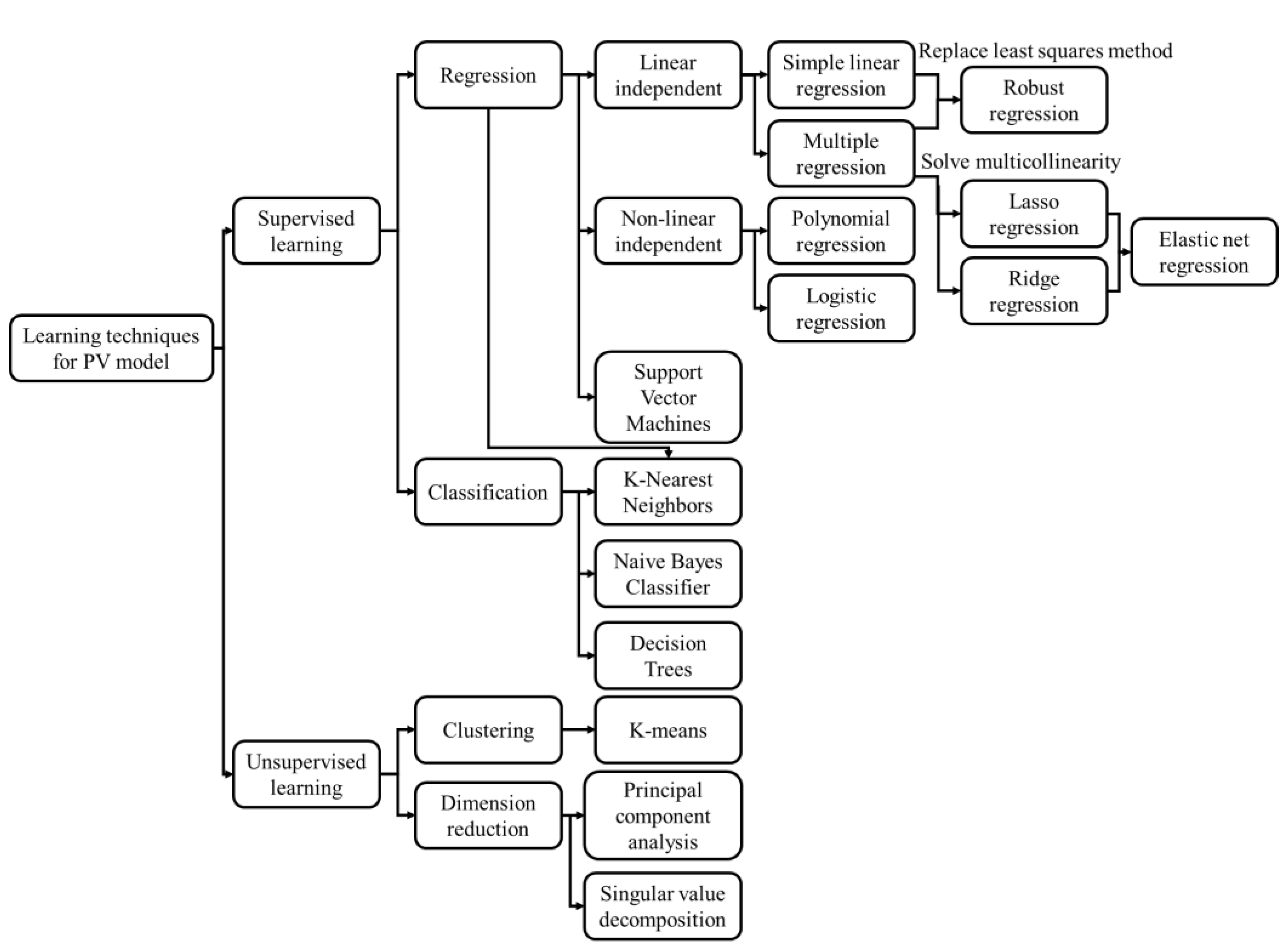
2. Learning Techniques for PV Power Forecasting Models

Machine learning models can be classified into four major types that are shown in Figure 1: supervised learning, unsupervised learning, semi-supervised learning, and reinforcement learning. For PV power forecasts, supervised learning and unsupervised learning are most used. Figure 2 shows a tree diagram that describes four major types of machine learning algorithms for solar power forecasting models.

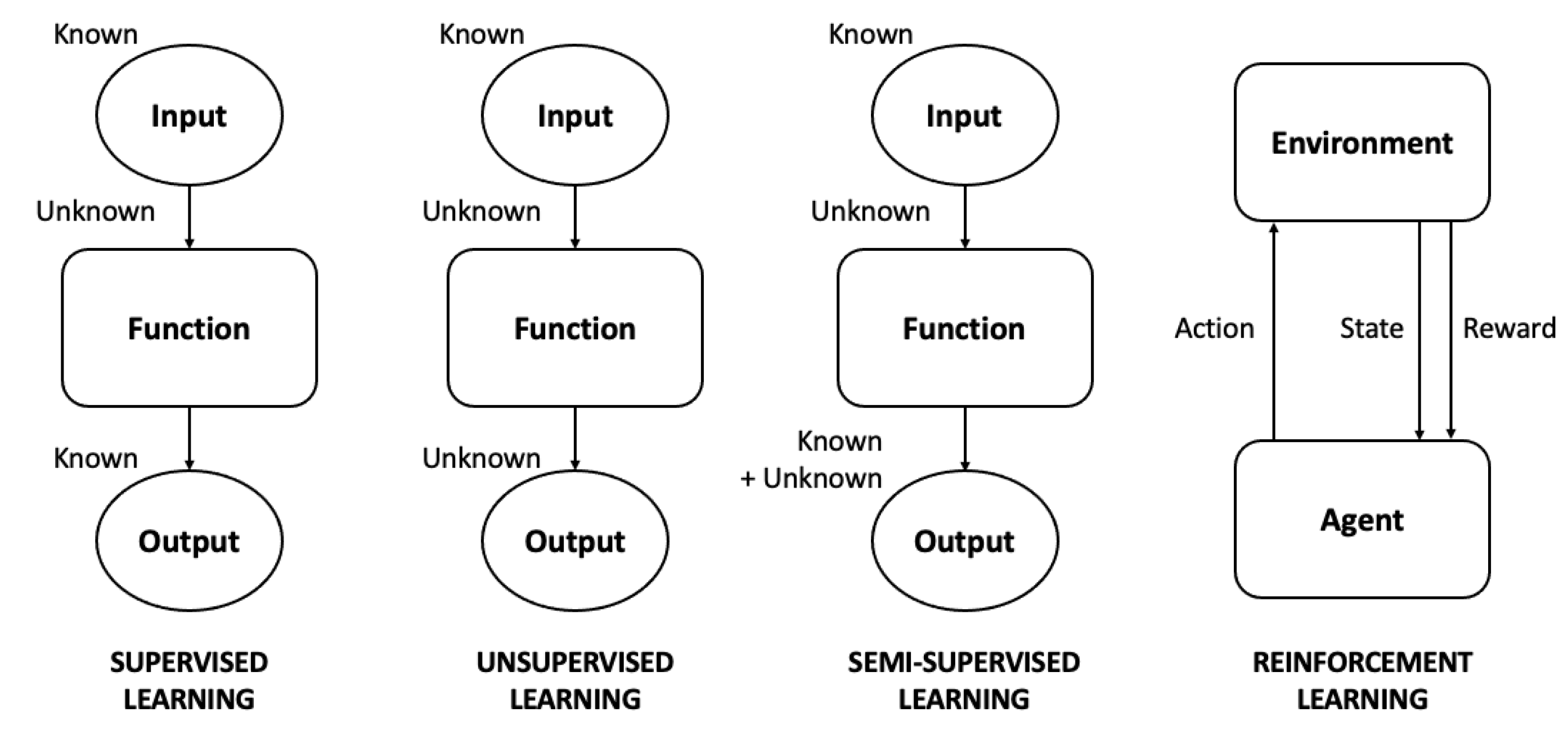
2.1. Supervised Learning

In supervised learning, the algorithm is trained from labeled datasets, they then classify or predict the corresponding value accurately. Supervised learning can be divided into two categories: classification and regression. Regression explores the relationship between independent variables (target values) and dependent variables (predicted values), which is very common in predictions and other analyses.
Regression can be divided into several types, the purpose of which is to minimize the distance between the data and the regression line. As the residual between the predicted value and the actual value decreases, then the sum square error (SSE) of the data is close to zero, which is called the least squares method. However, the outliers in the data affect the linear regression, and would lead to inaccurate predictions. Simple linear regression has only one independent variable and one dependent variable, and the regression line is a straight line. Multiple regression [17] also discusses the relationship between independent variables and dependent variables, but a multiple regression has more than two independent variables, so there is the problem of multicollinearity. Since not all independent variables and dependent variables are linearly related, a polynomial regression [18] with a higher-order nonlinear function can be used to obtain a lower error. In addition, logistic regressions [19] are supervised learning and classification algorithms that are used to determine the state of an event, then can predict the probability of a target variable. They provide other methods to deal with nonlinear functions. Most of the above regressions minimize the sum square error, but logistic regression generally uses the maximum likelihood estimation (MLE) to obtain its coefficients. To solve the problem of multicollinearity in multiple regression, two methods have been proposed: Lasso regression [20] and Ridge regression [21]. Lasso regression uses L1 regularization to normalize the loss function. This method can be used for feature selection because it is easy to generate a sparse matrix. Ridge regression uses L2 regularization to normalize the loss function, which can be used to prevent overfitting problems. An elastic net is the combination of Lasso regression and Ridge regression, which can handle feature selection and overfitting problems.
As outliers are in the data, the straight line/curve of linear regression would be affected, resulting in inaccurate predictions. Thus, Robust regression [22] can be used to replace the least-squares method. It uses a parameter of breaking point to set how many outliers can be accepted in the data without affecting the regression curve. Therefore, outliers outside the acceptable range are excluded from the training data.
Support vector machines (SVM) [23] can be used to solve both regression and classification problems. When the training data are in the same plane (hyperplane), SVM algorithms aim to find the decision boundary of the pre-classified data and maximize the boundaries between the pre-classified data. SVM performs well when the amount of inputs is less. However, large input data and outliers affect the classification results. SVM has been proven to have good performance in PV forecasting. JG da Silva Fonseca Jr. et al. [24] used SVM to pre-process input data that included normalized temperature, relative humidity, low level cloudiness, mid-level cloudiness, upper-level cloudiness, and Extraterrestrial insolation. The results show that SVM provides better forecasting results.
The K-Nearest Neighbors (K-NN) algorithm [25] is also a kind of supervised machine learning algorithm that takes classification and regression into account. It classifies the data through the similarity of recognition markers (such as the distance function) and then predicts the category of new data. K-NN belongs to the multi-classification method, and its classification performance is better than SVM. The calculation of K-NN becomes significantly heavier as the amount of input data increase. However, outliers in the data create little effect on the results, so it is suitable to classify rare events. X Luo et al. [26] used K-NN to classify weather types, which effectively improved the accuracy of predictions.
A Naive Bayes Classifier (NBC) [27] uses Bayes’ theorem to calculate the probability of each specific event, and takes the highest probability as the category. The equation is shown as follows.
P A | B = P ( B | A ) P A P B
where P(A) is the probability of occurrence of event A, P(B) is the probability of occurrence of event B, P(A|B) is the probability of event A when event B occurs, and P (B|A) is the likelihood that is the probability of predictor given class. The NBC model is simple, fast, and useful for big data. However, the algorithm judges the content of events; thus, the way to state events has a great effect on training performance.
Decision trees is a classification algorithm, which consists of root nodes (original data), internal nodes (feature judgment), and leaf nodes (decision result) [28]. The internal nodes decide the features to judge the original data, and then select the data with a high correlation of features. This method easily causes overfitting. Using decision trees to filter and obtain results is faster, and it can also deal with the problems caused by outliers.

2.2. Unsupervised Learning

In unsupervised learning, AI algorithms distinguish and classify the datasets containing non-labeled data. The common unsupervised learning includes clustering and dimension reduction algorithms.
K-means clustering [29] is one of the simplest and popular unsupervised learning algorithms. First, the data are divided into several groups, and the positions of each group are randomly assigned in the data. The data close to each group are classified into the same group, and the above actions are repeated until the positions of each group remain unchanged. K-means clustering may cause convergence to the local minimum. If outliers exist in the data, it is easy to produce deviations. To deal with large-scale data, the convergence speed by K-means clustering would be slow. H Zhang et al. [30] proposed a PV forecasting method with K-means clustering and can reduce the mean absolute percentage error (MAPE) by approximately 10%.
Principal component analysis (PCA) is a dimension reduction algorithm [31]. Through spatial mapping, the dimension of original data is mapped to a lower dimension, such as two or one dimensions. The dimension reduction method can extract the main information, and then remove noises, making the data easier to learn. Although reducing the amount of data is useful, information loss is a necessary part of PCA. Pierro et al. [32] used PCA to retain the relative humidity information of the weather forecasts and effectively reduced the space of the model inputs.
Singular value decomposition (SVD) is also a dimensionality reduction algorithm [33]. It used matrix operation to find individual eigenvalues and eigenvectors. Its target is also to achieve the feature decomposition in the dimension reduction algorithm.

3. Pre-Processing Methods

While collecting data, historical measurement data from PV sites may contain significant numbers of outliers, noises, or missing data. The input data directly affect forecasting results; as a result, the preprocessing of datasets is a critical step in PV forecasts that can improve the models’ performance. The methods of data pre-processing are summarized in Figure 3.

3.1. Data Cleaning

Abnormal data will lead to the deviation of the prediction results. The technique of data cleaning is mainly to fill or remove unnecessary information from a database [34]. If the missing rate is high and the importance is low, the data can be deleted. The linear internal difference method or the average method were widely used to handle missing values.

3.2. Normalization

Normalization is used to scale the original data to [0, 1] without changing its distribution [35]. The advantage of this method in data processing is that it can get rid of the limitation of data units on the model, speed up the convergence, and shorten the training time.

3.3. Z-Score Standardization

Standardization can transform the data into a normal distribution, in which the average value is zero and the standard deviation is unity [36]. The advantage of this method in data processing is to improve the convergence speed and forecasting accuracy. If a data distribution is close to the normal, the standardization is meaningful. However, if a data distribution is not close to the normal, the standard deviation causes the deviation of standardization. In addition, the influence of outliers can be reduced through Z-score normalization when the maximum and minimum outliers of the data cannot be determined. The formula is shown as follows.
z = x x m e a n x s t d
where x is the original data, xmean is the average value of data, and xstd is the standard deviation value of data.

3.4. Wavelet Transform (WT)

Typical time series can be handled by time domain-based or frequency domain-based methods. Based on time domain methods, a time series is regarded as the sequence of ordered points, and then the correlation among those points is analyzed. Based on frequency domain methods, the time series is converted to spectrum, and then the spectrum is analyzed as features. WT is a method to transfer data into time domain and frequency domain features, and then forward to the mother wavelet [37]. WT can indicate existing frequencies with the corresponding frequency occurrence. In addition, the outliers in the data have little effect on the forecasting results. However, once the basis function is determined, the whole calculation process cannot be replaced, indicating the lack of adaptability. M Zolfaghari et al. [38] used WT to decompose the input data into high-frequency and low-frequency sequences, and the prediction result shows that WT can improve the prediction performance.

3.5. Empirical Mode Decomposition (EMD)

EMD is based on the time-domain processing [39]. WT needs to select the mother wavelet first and cannot be replaced. In contrast, EMD can directly decompose the original time series into several intrinsic mode functions (IMFs) and a residual. The IMFs represent frequency components in the original time series, and they are arranged in order from high frequency to low frequency. This method is self-adaptive and can decompose non-linear and non-stationary signals directly without selecting basis functions. However, there is a problem about mixed modes in the IMF components. For instance, if the same IMF components appear at different times, it leads to the loss of physical significance of IMF. Shibo Wang et al. [40] used EMD to decompose wind speeds into IMFs with different proportions, and then built a prediction model for each sub-sequence.

3.6. Singular Spectrum Analysis (SSA)

SSA is a method to deal with nonlinear time series [41]. It can embed, decompose, group, and reconstruct the long-term trend, periodic signal, and noises of time series. In the process of analyses, embedding arranges a time series into a trajectory matrix, and SVD is used to decompose the time series to obtain the component matrix corresponding to each singular value. Finally, each group of components is reconstructed into a new time series. SSA was widely used in the fields of climate, environment, finance, etc. Yachao Zhang et al. [42] used SSA technology to obtain the hidden features of wind power generation.
Notably, data collection is a large challenge in solar power forecasting. One reason for this is that many solar sites do not install meters to measure solar irradiance, and even when measuring devices have been installed on site, instances of missing and incomplete data continue to occur. Therefore, strategies and practical methods to overcome these issues need to be proposed. The problem of missing data must be addressed at the preprocessing step by incorporating missing data imputation. The use of satellite imagery can also help to evaluate solar irradiance in real time, which could rectify to some degree the limited data collection possible at PV sites where irradiance meters have not been installed.

4. Classification of PV Power Forecasting Methods

Several methods and algorithms have been developed in the field of PV forecasts. They include two main categories: physical methods and statistical methods. The methods of PV forecasts are as summarized as Figure 4.

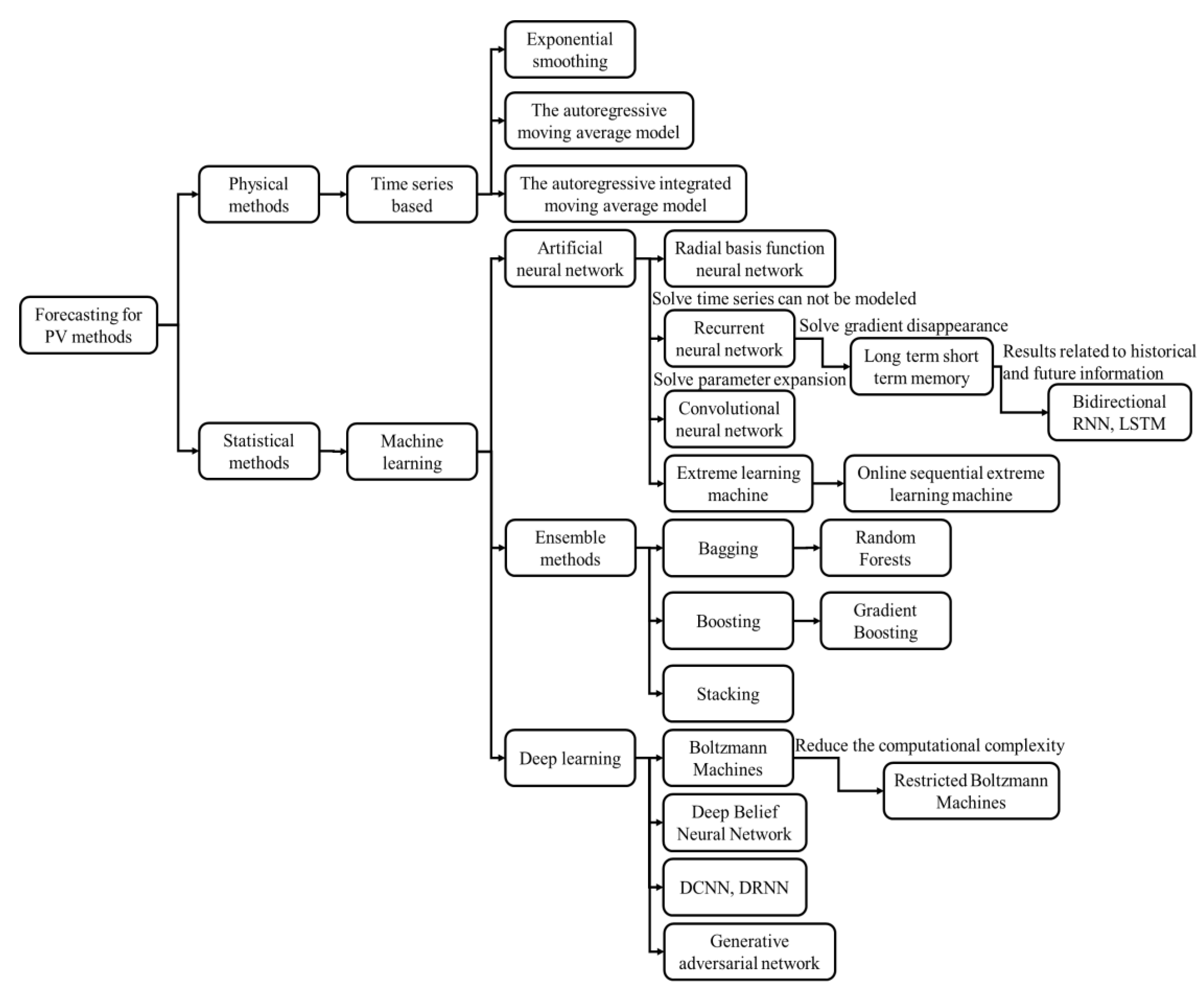
4.1. Physical Methods

Physical methods provide forecasts through the values of the atmospheric factors that are directly related to solar power generation [43]. These methods use meteorological data from NWP such as solar irradiance, rainfall, temperature, humidity, air pressure, wind speed, topography, etc. NWPs can be obtained by different forecasting modes, including the Weather Research and Forecasting Ensemble Prediction System (or called WEPS), Deterministic Weather Research and Forecasting (or called WRFD), or Radar Weather Research and Forecasting (or called RWRF) [11]. NWP is suitable for forecasting weather within a few hours or days and does not require any historical data. However, NWP is dependent on the stability of meteorological conditions, and physical models for NWP are difficult to be established.

4.2. Statistical Methods

Statistical approaches use historical data to define the correlation among them. These approaches do not need to provide atmospheric physical parameters. Therefore, the most important factor for such a forecasting model is the quality of the historical data. Subcategories of these methods include timeseries-based approaches and machine learning-based approaches.

4.2.1. Time Series-Based Methods

Time series-based methods investigate data features and regular patterns of historical data. The advantage of these methods is that they are not affected by external factors, but when the input data are unstable, the forecast error becomes larger.
The exponential smoothing method is a kind of weighted average method. This method gives a large weighting to the historical data that are closer to the forecasting data. In turn, the more distant historical data have less weights, and the weighting increases exponentially from far to near. These methods were commonly used for short-term or medium-term forecasts [44].
The autoregressive integrated moving average model (ARIMA) is a mixture of an autoregressive model (AR model) and a moving average model (MA model). The AR method uses the relationship between historical and real-time data to calculate a weighted average of past data to predict itself [45]. If the autocorrelation coefficient is less than 0.5, the prediction result would be inaccurate. The MA method is a weighted average of the random errors in AR. The random error is related to the random error generated in the past, which effectively eliminates the random fluctuation in the prediction. In the ARMA method, the errors ignored in the AR method are added to the MA method to make further adjustments. The ARIMA model converts a non-constant sequence into a constant sequence through the differential processing method [46], and then predicts it through the ARMA model, expressed as ARIMA (p, d, q), where d is the number of differences.

4.2.2. Machine Learning

Machine learning (ML) is a related AI application. Some popular ML forecasting models used in solar power applications are an artificial neural network (ANN), a long short-term memory (LSTM), a random forest (RF), a K-NN, an SVR, etc. An ANN is the most basic architecture of machine learning [47]. An ANN is based on a set of connected artificial neurons, like human brain neurons, and each connection can transfer signals to other neurons. A basic ANN structure comprises input, hidden, and output layers, also known as a multi-layer perceptron neural network (MLPNN). Neurons at the input layer pass information to neurons at the hidden layer by activation functions. A nonlinear training function is used to process information and interconnects each layer. The signal at each layer of neurons can only move forward, so it is called feed-forward neural networks. ANNs are often use in meteorology, finance, physics, engineering, and medicine. However, ANNs have the problems of parameter expansion, the phenomenon of overfitting, and the inability to model the changes in time series. An ANN has been developed to derivative methods to make the forecasting methods more suitable in different fields, for example: a radial basis function neural network (RBFNN), a convolutional neural network (CNN), a recurrent neural network (RNN), an LSTM, an extreme learning machine (ELM), and an online sequential extreme learning machine (OS-ELM).
An RBFNN has three layers: an input layer, a hidden layer with a non-linear activation function, and a linear output layer [48]. The training speed of an RBFNN is fast because of few hidden layers. However, the radial basis function graph is attenuation on both sides and radial symmetry. Thus, as the input data are very close to the center of data selection, it has a real mapping effect on the input, which is called local approximation.
A CNN has a good ability in spatial recognition; thus, many image recognition technologies are based on CNNs. A CNN uses a convolution kernel as a mediator [49]. The same convolution kernel is weight sharing in all images. By using a CNN, the number of network parameters (parameter expansion) and the complexity of the network can be reduced. Since the input data of CNNs have filters for defects, fault tolerance, and self-learning, it is helpful to obtain the correct feature values [50].
An RNN is a kind of neural network used to process sequence data. It is especially suitable for time series data. Different from a CNN, the output of an RNN in the hidden layer is recycled to the next hidden layer for training together [51]. Such a function ensures the correctness of input data. Since an RNN is a neural network that processes “time”, the problem of disappearance of the time gradient would occur when time is longer. However, RNN has short-term memory problems, and it cannot handle long input sequence data.
LSTM neural networks with long-term and short-term memories are a special type of RNN, which is a kind of architecture to prevent the gradient of long time series from disappearing [51]. Through the state of gates, the LSTM controls whether the input data transmit to the output, records the data that need to be memorized for a long time, and forgets the unimportant data. LSTMs can solve the problem of gradient disappearance caused by an RNN, but it fails to remove that problem completely. Moreover, an LSTM requires a long time and a large number of resources, which makes the model training more difficult.
A BRNN and a Bidirectional LSTM (BLSTM) are the continuations of RNN and LSTM methods, respectively [52]. Both RNN and LSTM neurons transmit information forward. However, bidirectional networks can pass forwards or backwards, indicating that the results are related to historical and future information.
An ELM is a learning algorithm for single-hidden-layer feedforward neural networks [53]. Different from the traditional feedforward neural network, the process from the input layer to the hidden layer of an ELM is random. There is no need to adjust the algorithm in the process of execution. In an ELM, the process from the hidden layer to the output layer only needs to solve a linear equation group; thus, the calculation speed can be improved. An ELM is usually unable to handle complex tasks, but it could perform well on simple tasks.
An OS-ELM is an advanced version of an ELM. An ELM needs to retrain and test new data, but an OS-ELM does not need this action. As new data arrives, an OS-ELM does not need to retrain the model with old data. It can insert data to the network to update the model continuously. However, since the structure of an OS-ELM is a single hidden layer network, it is difficult to effectively deal with complex applications even if a large number of hidden layer nodes are set. An OS-ELM is suitable for short-time learning but its performance for long-time learning is poor [54].
Most of the above models are suitable for short-term learning. However, many topics require long-term learning, which pushes the current development of long-term learning by statistical methods. Table 1 summarizes different types of artificial intelligence networks.
Ensemble methods integrate multiple identifiers into an identifier group to obtain a better and more comprehensive supervision model. The identifier can be trained separately, and then integrate multiple identifiers for overall prediction and evaluation. Common ensemble learning methods include Random Forests (RF), gradient boosting, bagging, stacking, and others.
Bagging is the abbreviation of bootstrap aggregating [55]. It randomly extracts the original data into several datasets, trains the datasets individually into a model, and finally classifies each model by voting or regressing the results. Under ideal conditions, the variance of the forecasting results is small.
An RF classifier is an integrated algorithm based on bootstrap aggregation (bagging) and decision trees [56]. This forest model is composed of many decision trees, and there is no correlation between each decision tree in the random forest. A bootstrap method is used to estimate the quantity of a population. This is done by the re-sample process to obtain the distribution of statistics and the confidence interval. The input data is randomly sampled. To avoid the overfitting problem, the data are randomly put into each decision tree to increase the extra randomness; then, each decision tree is classified. The mode is selected by voting, and the deviation is eliminated. In this way, the decision tree has diversity and can obtain better forecasts.
Boosting trains the original data for several rounds [57]. In each training, the model with a low error rate is given a higher weight. After sequential training, good classification results can be obtained. There are great differences between boosting and bagging training methods.
Gradient Boosting is a machine learning algorithm that integrates a weak learning model to promote its learning performance [58]. The promotion uses weak classifiers to reduce the last deviation. Unlike the bootstrap aggregation method, the lifting algorithm takes each output as the input of the next classifier to form a series. Bootstrap aggregation is a parallel training in each decision tree.
The bagging method extracts part of the data and uses the same method for training, but stacking uses different classifiers to train the data and builds the results into a dataset, which contains both a prediction and the actual results [59]. Then, the dataset is trained into a meta-classifier individually. Finally, the final result is obtained from the meta-classifier. Stacking can make the prediction better.
The summary of ensemble methods is shown in Table 2.
Traditional ANNs have less hidden layers, also known as shallow neural networks. Further, adding hidden layers and different algorithms makes the structure of ANNs more complex. The model can learn from a large number of input data and become deep learning, also known as a deep neural network (DNN). Common deep learning structures include Boltzmann machines, restricted Boltzmann machines, a generative adversarial network (GAN), a deep belief neural network (DBNN), and others.
A Boltzmann machine is an energy-based model [60]. The neurons of Boltzmann machines are fully connected, which causes a huge amount of calculation, so it is not often used. To reduce the computational complexity of Boltzmann machines, a new method called Restricted Boltzmann machines was designed [61]. It has only two layers: the input and hidden layers. The neurons in the same layer are not interconnected. The forward or backward transmission between different layers is determined by stochastic decisions. In this way, the data are continuously transmitted back and forth until the error between the input and output data is minimized. This process is called reconstruction, which is very suitable to put unlabeled data as inputs to obtain the characteristics of data, so an RBM is also an unsupervised learning.
DBNNs [62] stack multiple layers of Restricted Boltzmann machines and add a classifier to the last layer. Through this multi-layer unsupervised learning, a better forecasting result by classifying the pre-processed data can be obtained.
GANs are mainly composed of two CNNs, namely, a discriminating network and a generative network. The generative network randomly extracts data from the input, and its output is similar to the real data in the training set as far as possible. The input of the discriminating network is the output of the generative network. The purpose is to distinguish the output of the generative network from the real data as much as possible and check whether the data are reasonable. GANs have been widely used for data generation, such as image and video generation, synthesis, recognition, etc. [63].

4.2.3. Deep Learning

In classical machine learning models such as AR, feature engineering is performed manually, and parameters of the models need to be optimized. Deep learning models learn features directly from datasets, which can learn more complex patterns of data and improve the training speed. The use of deep learning for PV generation forecasting overcomes the traditional machine learning disadvantages.
The Gated Recurrent Unit (GRU) is a new generation of RNNs. Similar to LSTMs, GRUs use an update gate and a reset gate to solve the vanishing problem of RNNs. These gates can be trained to keep information from the previous time steps and to remove information that does not affect the forecasting accuracy. GRUs can perform better than LSTMs in terms of speed and the number of parameters [64]. In [65], a short-term PV power forecasting based on GRUs is proposed, which can effectively consider the influence of features and historical PV power on the future PV power output.
The encoder–decoder model for RNNs was introduced to simplify the seq2seq mapping models [66]. It uses a deep neural network such as an RNN or an LSTM to encode the input into a fixed vector, and then uses another deep neural network to decode the fixed vector into the sequence output. An encoder–decoder model can map sequences of different lengths to each other. However, it only works well for small sequences as it is difficult to transform a long sequence into one vector when the length of input sequence increase.
To solve the long input sequence problem of encoder–decoder models, an attention mechanism is developed. The encoder–encoder with an attention mechanism first learns the weight of each element from the input sequence, then recombines the elements by weight. Attention mechanisms can drop the unimportant information and focus more on the useful information from the input data. However, attention mechanism models are mostly used in the field of image and natural language processing issues. In 2017, the Google research team introduced a Transformer based on an attention mechanism [67]. The core of the Transformer is also an encoder–decoder. In PV generation forecasting, the model is treated as a black box, input data are historical measured PV power and other meteorological variables, and the output is forecasting a PV generation value. In the Transformer, an encoder block contains a self-attention layer and a feed-forward neural network. The decoder block has the same structure as the encoder block and has an additional layer called the encoder–decoder-attention, which analyzes the relationship between the current forecasting value and encoded feature vector.
To enhance the performance of self-attention-based models, there are some research works such as: the Sparse Transformer [68], LogSparse Transformer [69], Longformer [70], the Reformer [71], Linformer [72], Transformer-XL [73], and Compressive Transformer [74]. The structure of Informer includes the encoder part and the decoder part, with the main purpose is to solve long time-series problems in forecasting tasks. The informer receives a long sequence input, and the self-attention block of the Transformer is replaced by a multi-head ProbSparse Self-attention [75]. To reduce the size of the network, Informer uses self-attention distilling. The decoder also receives long sequence inputs, measures the weighted attention composition of the feature map, then immediately forecasts the output values through a fully connected layer. By using ProbSparse Self-attention and self-attention distilling, the Informer can improve the computational complexity overall.

5. Major Factors Affecting Solar Power Forecasting

As discussed in earlier chapters, the input data quality has a significant impact on forecasting accuracy. The range of the forecasting horizons, weather classification, missing data, and outliers contribute to the data quality. The input variables that influence solar power predictions are summarized as follows.

5.1. Forecasting Horizons

Forecasting horizons refers to the time length for forecasting PV generation in the future. The accuracy of a PV forecasting model depends on the forecasting horizons. Therefore, according to the forecasting purpose, one can consider which model is suitable with a certain forecasting horizon. The time range of short-term is generally defined as several minutes or several hours. The application of short-term PV forecasts ensures power system stability and security. The forecasting horizons of medium-term is generally defined as one or several days. The application of medium-term PV power forecasts is for maintenance plan. The long-term forecasting horizon is generally defined as more than one week. Its applications are also for power system maintenance and operation. However, the accuracy of long-term forecasts is relatively low because the consideration of factors in this forecasting are more complex.

5.2. Weather Classification

The reason why solar energy is unstable is mainly due to the interference of the weather. As the sun is shaded, the power generation drops sharply, causing troubles in grid dispatching. Therefore, weather inputs play important roles in the forecasting model. The factors that affect or are related to sunlight include sunshine amount, atmospheric temperature, module temperature, wind speeds, humidity, atmospheric pressure, cloud type, etc. Thus, some literatures analyzed the relationship between related factors and PV power generation. However, solar irradiance is the most important variable that affects solar power generation [76].

5.3. Optimization of Model Parameters

Various optimization algorithms have been used in PV forecasting models, and the model inputs can be determined appropriately to improve the forecasting accuracy. Optimizing algorithms can solve a wide range of problems by designing suitable algorithms for different problems. Good quality and efficiency can be obtained when the complexity of the problem is high, the scale is large, and the characteristics are not clear. Many literatures proposed various optimization algorithms for PV power forecasts, which includes a genetic algorithm (GA) [77], particle swarm optimization (PSO) [78], a grid-search [79], the firefly algorithm (FF) [80], ant colony optimization (ACO) [81], the fruit fly optimization algorithm (FOA) [82], the artificial bee colony (ABC) [83], the charged system search (CSS) [84], etc.
The operation of a GA is similar to natural selection in terms of achieving the optimal results, which means that the fittest survive and the unfit are eliminated. However, as dealing with big data, the amount of calculation by a GA is quite large. An ACO algorithm process is the same as ants searching for food by observing the footprints. When searching for food, ants communicate which path is the most suitable through pheromones and continue to update to the best path. Since ants can exchange information with each other by using pheromones, ACOs would have a better ability to find the global optimal solution. The PSO algorithm was developed by observing the behavior of birds looking for food. Each particle represents a bird, which has memory and reference. Generally, the calculation process by the PSO is based on experience, and it is difficult to avoid the problem of the local optimal solution. The FOA was developed by observing the behavior of fruit flies looking for food. This method is simple in the low dimension, but for data processing in the high dimension, the convergence speed of iteration is slow, and the accuracy is low. The grid search is a method to adjust parameters for optimization. In each case, exhaustive searching is performed, and different parameters are tried to obtain the best result. This method is suitable for a small number of parameters. A large number of parameters would be very time-consuming for computation.
The FF was developed through the characteristics that fireflies emit light and attract each other. First, the algorithm sets the firefly position and brightness. In the definition, the mutual attraction of fireflies is directly proportional to the luminous brightness, and the brightness is inversely proportional to the distance; thus, the firefly with a brighter brightness may attract other fireflies. However, if the brightness is the same, it moves randomly. As the maximum number of iterations is reached, the final position of the firefly is the result.
The ABC algorithm was developed by observing the behavior of bees looking for food. The main parameters of this algorithm are leader, scout, follower, and food source. The leader has a memory of food location, storage capacity, collection difficulty, etc. It will have the opportunity to share the information to the follower. The follower selects food sources to collect and updates the food source information. Finally, the scouter searches for food locations nearby and updates honey source information. By iterating the above steps repeatedly, the local optimal solution can be found through each bee, and then the global optimal solution can be obtained.
The CSS is a randomized algorithm based on Coulomb’s and Newton’s theorem. Each charged particle (CP) is assigned a random position, and the fitness values of each CP are calculated. The best fitness values are arranged in order, and the first quarter of fitness values are selected to store in charge memory storage (CM). Then, the probability of each CP moving, and the resultant force can be calculated. This algorithm continuously updates the new position and speed of CPs after moving until the maximum number of iterations is reached. The final fitness values are the global optimal solution.

5.4. Performance of Forecast Models

Common indexes for evaluating deterministic forecasting performance include the mean square error (MSE) [85], the mean absolute error (MAE) [86], the root mean square error (RMSE) [86], the normalized root mean square error (nRMSE) [35], and the mean absolute error percentage (MAPE) [87]. The mean square error squares all the errors between the predicted values and the actual values, and then adds them together to obtain the average value to evaluate the variability of the values. Compared with the mean square error, the mean absolute error uses absolute values instead of the maximum outlier after the square. Therefore, the mean absolute error could reflect the actual situation about forecasting errors. The root mean square error, also known as the standard error, can reflect the accuracy of the value very well if the error is not obvious. The normalized root mean square error (nRMSE) normalizes the value of the root mean square error into (0, 1). It is often used to evaluate the similarity between two signals and the overall deviation. The mean absolute percentage error (MAPE) takes the absolute value of the MPE (mean percentage error) and then adds the percentage. Since the actual value is the denominator, the MAPE is generally used when the actual value is not zero. An appropriate error measurement can be selected based on different conditions. The MAPE, for example, cannot be utilized if the time series contains zero. Furthermore, the MAE, MSE, and RMSE are the evaluation methods that are usually influenced by outliers.

6. Hybrid Models

If only one forecasting model is utilized, forecasting results would not be good enough. Therefore, hybrid models have been applied in many forecasting works. The structure of a hybrid model is a combination of two or more forecasting models that overcomes a single model’s technical constraints and enhances the predicting accuracy. Table 3 summarizes various hybrid methods in recent years.

7. Probabilistic Forecast Techniques

Recently, numerous studies have focused mostly on deterministic forecasts, often known as a single-value forecasting. Since PV generation is intermittent energy and full of uncertainties, deterministic forecasts could not satisfy the requirement of power system operations. To estimate PV power generation with a possible range, probabilistic predictions must be applied. The methods of probabilistic forecasts include lower upper bound estimation (LUBE) [90], probability density function (PDF) [99], cumulative distribution function (CDF) [100], prediction interval coverage probability (PICP) [101], prediction interval normalized average width (PINAW) [101], coverage width criterion (CWC) [7], continuous rank probability score (CRPS) [102], and CRPS skill score (CRPSSS) [103], etc.
PDF is one of the core concepts in probability theory, which is used to describe the probability distribution of the corresponding output. It allows users to fully understand all potential ranges and probabilities of future-observed data, and then present a more accurate forecast. However, in the application of continuous data, typical probability distributions include continuous uniform distribution, normal distribution, gram distribution, etc., in which statistical data are based on known samples to set a group of parameters. Continuous uniform distribution means that the probability of values in an interval is equal, and the probability of values falling outside the interval is zero. Normal distribution is also known as Gaussian distribution. A normal distribution indicates that the probability of data is the largest in the mean value, and the distribution is almost within three standard deviations. Gramma distribution is used for data with an asymmetric distribution. As the shape parameter is larger, the gramma distribution tends to be a normal distribution. The larger the scale parameter is, the more divergent its distribution is. The nonparametric method means that the statistical data are not clear, so the parameters cannot be fixed. The nonparametric methods are used when the parametric methods cannot be used.
The integral of probability density function that may completely capture the probability distribution of a real random variable is known as CDF. Both CDF and PDF are capable of being converted to each other.
The evaluation of probability forecasting results typically includes two components: reliability and sensitivity. The ability of the forecasted lower upper bound estimation to cover the actual confidence interval is represented by reliability, and its evaluation index is called PICP. To archive good reliability, PICP should be as close as possible to the actual confidence interval. In addition, sensitivity denotes the accuracy with which the lower upper bound is estimated, and its evaluation index is called PINAW. A small PINAW represents that the forecasting model is more accurate. Using CWC, one can evaluate PICP and PINAW together and obtain the model’s performance score. A small CWC represents that the performance of the prediction model is better.
CRPS is evolved from the Brier score, which calculates the prediction error with probability. CRPS is regarded as a score to predict the accuracy of CDF by integrating the difference between all possible thresholds and probabilities. CRPSSS further evaluates the prediction ability of CRPS. To compare with CRPS, a reference CRPS (RCRPS) is also required. RCRPS can be used in deterministic forecasts. If CRPSSS is bigger than zero, the system has prediction ability. If CRPSSS is equal to unity, it is the best case.

8. Discussions

8.1. Important Findings from Literature Reviews

Forecasting models make use of a variety of parameters. For instance, an ARIMA model includes different order AR or MA parameters. These parameters can be obtained using optimization algorithms; however, there is no single algorithm that can be used in all forecasting cases. Different optimization methods can be applied suitably to different statistical or machine learning models. The major factors that affect forecasting accuracy include the selection of the input variables, the type of data processing employed, the appropriateness of the learning models, and the weather classification. In recent years, several data preprocessing techniques have received a large amount of attention, especially those related to data cleaning and normalization. Several feature extraction technologies have also been used, including Wavelet Decomposition and Empirical Mode Decomposition, which are the most commonly used methods. It has also been observed that supervised learning methods have been used more frequently than unsupervised methods, and that there is a trend towards the mainstream use of novel deep learning structures, despite some studies still using time-series based methods. Weather classification is significant for day-ahead PV forecasts, and the concept is analogous to that in the Similar Days short-term load forecast. Finally, it is remarked that hybrid models that integrate physical models with statistical methods remain the primary forecasting tool for PV power forecasting.
Different input data and models should be selected for different forecasting purposes; however, it is exceedingly difficult to compare the forecast performance that results from the selection of these different forecasting models, PV sites, input variables, and forecasting lead times because the environmental characteristics of each PV site, the selected input variables, and the lead time of the forecasts are completely different. Nevertheless, several significant findings can be summarized as follows:
  • The forecasting horizon has a strong influence on forecasting accuracy. When the lead time is shorter, the average forecasting error is smaller.
  • The majority of PV forecasts use the inputs of solar irradiation, atmospheric temperature, and wind speed, but some use advanced input variables such as global horizontal irradiance, diffused horizontal irradiance, diffused normal irradiance, and total cloud cover.
  • Site-related parameters such as the solar zenith angle are also considered in some papers.
  • Different statistical methods can be used to evaluate the performance of the forecasting models, among which the MAE, the MSE, and the RMSE are the most popular indexes.
  • Machine learning-based methods that employ optimization parameter searching have been the most popular methods in recent years. Optimizing the model parameters and selecting appropriate input data effectively improves the accuracy of the forecasting model.

8.2. Knowledge Gaps

The following knowledge gaps have been identified and require further research:

8.2.1. The Integration of Atmospheric Science with Renewable Power Forecasting

The adoption of atmospheric science for renewable power forecasting has historically been fairly weak. Atmospheric science has traditionally focused on the forecasting of extreme wind speeds (e.g., typhoons), rainfall, and temperature and paid less attention to solar irradiance, and yet accurate forecasting of solar irradiance is essential for the accurate forecasting of PV power. Therefore, the application of Numerical Weather Prediction (NWP) to solar irradiance should be promoted. A first step in this direction has been the recent development of the WRF-Solar NWP model for PV applications globally.

8.2.2. The Restricted Application of Novel AI Models

Novel deep learning and machine learning models are developing quickly; however, these models have thus far been limited in their use to the fields of computer science and image processing. Thus, there appears to be a large number of applications to which these AI models have not yet been implemented and PV power forecasting is certainly one application where they could prove very effective, although further research is required on this matter.

8.2.3. The Selection of the Optimal Combination of Data Collection Tools

PV power forecasts rely on various tools to collect input data. These tools include solar irradiance meters, numerical weather predictions, sky image meters, and even satellite imagery. Different tools can be suitable for different purposes or for different lead times during the forecasting process. Therefore, the selection of different combinations of these tools is an important step in the forecast process as employment of the appropriate tools would significantly increase efficiency.

8.2.4. The Implementation of a Cross-Disciplinary Approach

The generation of PV forecasts requires a cross-disciplinary approach, combining atmospheric science, mathematical statics, computer science, machine learning, and power engineering to give one example. This combination of different fields of knowledge in the construction of the forecasting engine is crucial in ensuring the quality of the forecasts it can generate.

8.2.5. The Stability of Data Collection

Stable data collection is very useful in the establishment of a forecasting module; however, most PV measurements are missing data or contain noise. Thus, enhancing measurement stability, including the improvement of data-collection techniques and the imputation of missing data, is a task that would yield considerable fruit.

8.3. Future Scopes

Tremendous progress has been made in the fields of atmospheric science, computer science, measurement science, and artificial intelligence in recent years. Thus, the uncertainty in renewable power generation can be greatly reduced by using accurate prediction technologies. Important issues in PV forecasting include numerical weather prediction, data processing, and statistics-based and artificial intelligence-based training models. Numerical weather prediction can predict a few hours or days in the future a variety of atmospheric parameters such as wind speed, insolation, rainfall, temperature and humidity, air pressure, etc. In addition to NWP, various auxiliary tools such as satellite imagery, sky imagery, and wind speeds measured using lidar can also assist in obtaining important input data for PV forecasting models. These selected inputs are the core data for prediction. During the forecasting process, however, input data may be missing or contain significant noise, which renders them inappropriate for direct use in model training. Thus, data preprocessing is a vital step required to maintain high-quality data. It can reduce or filter noise to a significant degree, fill in missing data, and extract the main features of the original data. Typical preprocessing techniques include data cleaning and standardization, classification, regression, clustering, and dimensionality reduction. This last step is performed to complete the forecasting model.
Previously, a variety of statistical methods and traditional neural networks have been used to train forecasting models, but more recently many new AI models, and in particular those incorporating machine and deep learning algorithms, have been proposed and their popularity has continued to grow. The structure of a traditional neural network has relatively few hidden layers or neurons, but deep learning increases the number of hidden layers and the amount of feedback, thus creating a more complex learning structure. Incidentally, the major difference between deep learning and machine learning is that deep learning is a subset of machine learning that can learn valuable characteristics from a dataset automatically and then reduce computational time using parallel processes. Many new deep learning algorithms have not yet been used in solar power forecasting, for which they may prove to be very beneficial.
Traditional deterministic forecasting methods only provide a single value prediction. This means that they cannot offer flexibility to industrial applications, but an operating range that takes uncertainties into account is important for power system operations. As renewable power generation increases, the uncertainty of power generation in a system also increases and thus, probabilistic forecasting, stochastic unit scheduling, and probabilistic load flow become more important factors in power system operation. It is expected that there will be a clear trend towards probabilistic forecasts for PV power generation, and that these forecasting results will be applied to the decision making and risk management of power systems.
In summary, the complete process of solar power forecasting requires the collection of a large amount of data, the implementation of multi-dimensional data processing and feature extraction, and the application of a powerful deep learning structure for training.

9. Conclusions

PV power generation has an inherent problem of intermittency, which affects power system reliability. Therefore, it is essential to design reliable forecasting models for such systems. In this article, the techniques used for solar power forecasting are summarized in a systematic and comprehensive manner. The key topics identified from the survey were learning techniques, data processing, the classification of forecasting methods, major factors that affect the forecasting performance, and the estimation of forecasting uncertainties. It was observed that supervised learning methods were used more frequently than unsupervised methods and also that most forecasting methods applied a data cleaning and normalization process to reduce forecasting errors. Several feature extraction technologies were also used, including Wavelet Decomposition and Empirical Mode Decomposition, which were the most commonly used methods. Both statistical and hybrid models have been widely preferred over purely physical models, and machine learning was the most popular method used for PV forecasting. Of particular interest is the fact that various machine learning models that employ optimal algorithms have received an increasing amount of attention, with the more commonly used optimal algorithms being the PSO, GA, and WOA. The major factors that affect the forecasting results were identified as solar irradiance, wind speed, and temperature; and thus, they are naturally the more commonly used inputs. Although probabilistic forecasts with uncertainty information are highly useful for system operations, deterministic forecasts remain the primary methods used; however, it is expected that the importance of the former will increase.
The main contributions of this paper are to provide a complete overview of potential AI models for PV forecasting, and in particular an introduction to novel deep learning models based on attention mechanisms. These new deep learning algorithms were initially applied to image processing, and few have yet been used for PV power forecasting; thus, there is a huge reservoir of untapped potential in the application of these new deep learning models to time-series forecasts. In addition, the importance of data processing techniques to forecasting is emphasized since their appropriate use significantly enhances forecasting accuracy. Finally, this paper provides a comprehensive discussion of the suggested future scope of PV forecasting research as well as an identification of several gaps in our current knowledge.

Author Contributions

Conceptualization, Y.-K.W. and C.-L.H.; methodology, Y.-K.W. and C.-L.H.; software, C.-L.H. and Q.-T.P.; validation, Y.-K.W., Y.-Y.L.; formal analysis, C.-L.H.; investigation, C.-L.H.; resources, Y.-K.W. and C.-L.H.; writing—original draft preparation, C.-L.H., Y.-K.W., Q.-T.P. and Y.-Y.L.; writing—review and editing, Y.-K.W.; supervision, Y.-K.W. and Y.-Y.L.; project administration, Y.-K.W. All authors have read and agreed to the published version of the manuscript.

Funding

This work is financially supported by the Ministry of Science and Technology (MOST) of Taiwan under Grant MOST 110-3116-F-008-001. Project title: Research of Power Regulation and Field Implementation for Smart Multi-level Microgrid.

Institutional Review Board Statement

Not applicable.

Informed Consent Statement

Not applicable.

Conflicts of Interest

The authors declare no competing financial interests.

References

  1. Liu, L.; Zhao, Y.; Chang, D.; Xie, J.; Ma, Z.; Sun, Q.; Yin, H.; Wennersten, R. Prediction of short-term PV power output and uncertainty analysis. Appl. Energy 2018, 228, 700–711. [Google Scholar] [CrossRef]
  2. Shivashankar, S.; Mekhilef, S.; Mokhlis, H.; Karimi, M. Mitigating methods of power fluctuation of photovoltaic (PV) sources–A review. Renew. Sustain. Energy Rev. 2016, 59, 1170–1184. [Google Scholar] [CrossRef]
  3. Antonanzas, J.; Osorio, N.; Escobar, R.; Urraca, R.; Martinez-de-Pison, F.J.; Antonanzas-Torres, F. Review of photovoltaic power forecasting. Sol. Energy 2016, 136, 78–111. [Google Scholar] [CrossRef]
  4. Almeida, M.P.; Muñoz, M.; de la Parra, I.; Perpiñán, O. Comparative study of PV power forecast using parametric and nonparametric PV models. Sol. Energy 2017, 155, 854–866. [Google Scholar] [CrossRef] [Green Version]
  5. Lorenz, E.; Heinemann, D. Prediction of solar irradiance and photovoltaic power. Compr. Renew. Energy 2012, 1, 239–292. [Google Scholar]
  6. Ulbricht, R.; Fischer, U.; Lehner, W.; Donker, H. First steps towards a systematical optimized strategy for solar energy supply forecasting. In Proceedings of the European Conference on Machine Learning and Principles and Practice of Knowledge Discovery in Databases (ECMLPKDD 2013), Prague, Czech Republic, 23–27 September 2013. [Google Scholar]
  7. Phan, Q.T.; Wu, Y.K.; Phan, Q.D. A Hybrid Wind Power Forecasting Model with XGBoost, Data Preprocessing Considering Different NWPs. Appl. Sci. 2021, 11, 1100. [Google Scholar] [CrossRef]
  8. Antonanzas, J.; Pozo-Vázquez, D.; Fernandez-Jimenez, L.; Martinez-de-Pison, F. The value of day-ahead forecasting for photovoltaics in the Spanish electricity market. Sol. Energy 2017, 158, 140–146. [Google Scholar] [CrossRef]
  9. Theocharides, S.; Makrides, G.; Livera, A.; Theristis, M.; Kaimakis, P.; Georghiou, G.E. Day-ahead photovoltaic power production forecasting methodology based on machine learning and statistical post-processing. Appl. Energy 2020, 268, 115023. [Google Scholar] [CrossRef]
  10. Wang, R.; Li, J.; Wang, J.; Gao, C. Research and application of a hybrid wind energy forecasting system based on data processing and an optimized extreme learning machine. Energies 2018, 11, 1712. [Google Scholar] [CrossRef] [Green Version]
  11. Wu, Y.-K.; Su, P.-E.; Wu, T.-Y.; Hong, J.-S.; Hassan, M.Y. Probabilistic wind-power forecasting using weather ensemble models. IEEE Trans. Ind. Appl. 2018, 54, 5609–5620. [Google Scholar] [CrossRef]
  12. Ahmed, R.; Sreeram, V.; Mishra, Y.; Arif, M. A review and evaluation of the state-of-the-art in PV solar power forecasting: Techniques and optimization. Renew. Sustain. Energy Rev. 2020, 124, 109792. [Google Scholar] [CrossRef]
  13. Das, U.K.; Tey, K.S.; Seyedmahmoudian, M.; Mekhilef, S.; Idris, M.Y.I.; Van Deventer, W.; Horan, B.; Stojcevski, A. Forecasting of photovoltaic power generation and model optimization: A review. Renew. Sustain. Energy Rev. 2018, 81, 912–928. [Google Scholar] [CrossRef]
  14. Mellit, A.; Pavan, A.M.; Ogliari, E.; Leva, S.; Lughi, V. Advanced methods for photovoltaic output power forecasting: A review. Appl. Sci. 2020, 10, 487. [Google Scholar] [CrossRef] [Green Version]
  15. Akhter, M.N.; Mekhilef, S.; Mokhlis, H.; Shah, N.M. Review on forecasting of photovoltaic power generation based on machine learning and metaheuristic techniques. IET Renew. Power Gener. 2019, 13, 1009–1023. [Google Scholar] [CrossRef] [Green Version]
  16. Ellahi, M.; Abbas, G.; Khan, I.; Koola, P.M.; Nasir, M.; Raza, A.; Farooq, U. Recent approaches of forecasting and optimal economic dispatch to overcome intermittency of wind and photovoltaic (PV) systems: A review. Energies 2019, 12, 4392. [Google Scholar] [CrossRef] [Green Version]
  17. Trigo-González, M.; Batlles, F.; Alonso-Montesinos, J.; Ferrada, P.; Del Sagrado, J.; Martínez-Durbán, M.; Cortés, M.; Portillo, C.; Marzo, A. Hourly PV production estimation by means of an exportable multiple linear regression model. Renew. Energy 2019, 135, 303–312. [Google Scholar] [CrossRef]
  18. Mahmud, K.; Azam, S.; Karim, A.; Zobaed, S.; Shanmugam, B.; Mathur, D. Machine Learning Based PV Power Generation Forecasting in Alice Springs. IEEE Access 2021, 9, 46117–46128. [Google Scholar] [CrossRef]
  19. Dairi, A.; Harrou, F.; Sun, Y.; Khadraoui, S. Short-term forecasting of photovoltaic solar power production using variational auto-encoder driven deep learning approach. Appl. Sci. 2020, 10, 8400. [Google Scholar] [CrossRef]
  20. Yang, D. Ultra-fast preselection in lasso-type spatio-temporal solar forecasting problems. Sol. Energy 2018, 176, 788–796. [Google Scholar] [CrossRef]
  21. Li, T.; Zhou, Y.; Li, X.; Wu, J.; He, T. Forecasting daily crude oil prices using improved CEEMDAN and ridge regression-based predictors. Energies 2019, 12, 3603. [Google Scholar] [CrossRef] [Green Version]
  22. Jordan, D.C.; Deline, C.; Kurtz, S.R.; Kimball, G.M.; Anderson, M. Robust PV degradation methodology and application. IEEE J. Photovolt. 2017, 8, 525–531. [Google Scholar] [CrossRef]
  23. Zhang, W.; Zhang, H.; Liu, J.; Li, K.; Yang, D.; Tian, H. Weather prediction with multiclass support vector machines in the fault detection of photovoltaic system. IEEE/CAA J. Autom. Sin. 2017, 4, 520–525. [Google Scholar] [CrossRef]
  24. da Silva Fonseca, J.G., Jr.; Oozeki, T.; Takashima, T.; Koshimizu, G.; Uchida, Y.; Ogimoto, K. Use of support vector regression and numerically predicted cloudiness to forecast power output of a photovoltaic power plant in Kitakyushu, Japan. Prog. Photovolt. Res. Appl. 2012, 20, 874–882. [Google Scholar] [CrossRef]
  25. Harrou, F.; Taghezouit, B.; Sun, Y. Improved kNN-based monitoring schemes for detecting faults in PV systems. IEEE J. Photovolt. 2019, 9, 811–821. [Google Scholar] [CrossRef]
  26. Tan, J.; Deng, C. Ultra-short-term photovoltaic generation forecasting model based on weather clustering and markov chain. In Proceedings of the 2017 IEEE 44th Photovoltaic Specialist Conference (PVSC), Washington, DC, USA, 25–30 June 2017; IEEE: Piscataway, NJ, USA, 2017; pp. 1158–1162. [Google Scholar]
  27. Kwon, Y.; Kwasinski, A.; Kwasinski, A. Solar irradiance forecast using naïve Bayes classifier based on publicly available weather forecasting variables. Energies 2019, 12, 1529. [Google Scholar] [CrossRef] [Green Version]
  28. Ahmad, M.W.; Mourshed, M.; Rezgui, Y. Tree-based ensemble methods for predicting PV power generation and their comparison with support vector regression. Energy 2018, 164, 465–474. [Google Scholar] [CrossRef]
  29. Zhen, Z.; Liu, J.; Zhang, Z.; Wang, F.; Chai, H.; Yu, Y.; Lu, X.; Wang, T.; Lin, Y. Deep learning based surface irradiance mapping model for solar PV power forecasting using sky image. IEEE Trans. Ind. Appl. 2020, 56, 3385–3396. [Google Scholar] [CrossRef]
  30. Zhang, H.; Li, D.; Tian, Z.; Guo, L. A Short-Term Photovoltaic Power Output Prediction for Virtual Plant Peak Regulation Based on K-means Clustering and Improved BP Neural Network. In Proceedings of the 2021 11th International Conference on Power, Energy and Electrical Engineering (CPEEE), Shiga, Japan, 26–28 February 2021; IEEE: Piscataway, NJ, USA, 2021; pp. 241–244. [Google Scholar]
  31. Lan, H.; Zhang, C.; Hong, Y.-Y.; He, Y.; Wen, S. Day-ahead spatiotemporal solar irradiation forecasting using frequency-based hybrid principal component analysis and neural network. Appl. Energy 2019, 247, 389–402. [Google Scholar] [CrossRef]
  32. Pierro, M.; De Felice, M.; Maggioni, E.; Moser, D.; Perotto, A.; Spada, F.; Cornaro, C. Data-driven upscaling methods for regional photovoltaic power estimation and forecast using satellite and numerical weather prediction data. Sol. Energy 2017, 158, 1026–1038. [Google Scholar] [CrossRef]
  33. Prasad, R.; Ali, M.; Xiang, Y.; Khan, H., A. double decomposition-based modelling approach to forecast weekly solar radiation. Renew. Energy 2020, 152, 9–22. [Google Scholar] [CrossRef]
  34. Wang, Z.; Xu, Z.; Zhang, Y.; Xie, M. Optimal Cleaning Scheduling for Photovoltaic Systems in the Field Based on Electricity Generation and Dust Deposition Forecasting. IEEE J. Photovolt. 2020, 10, 1126–1132. [Google Scholar] [CrossRef]
  35. Massaoudi, M.; Chihi, I.; Sidhom, L.; Trabelsi, M.; Refaat, S.S.; Abu-Rub, H.; Oueslati, F.S. An effective hybrid NARX-LSTM model for point and interval PV power forecasting. IEEE Access 2021, 9, 36571–36588. [Google Scholar] [CrossRef]
  36. Arora, I.; Gambhir, J.; Kaur, T. Data Normalisation-Based Solar Irradiance Forecasting Using Artificial Neural Networks. Arab. J. Sci. Eng. 2021, 46, 1333–1343. [Google Scholar] [CrossRef]
  37. Alipour, M.; Aghaei, J.; Norouzi, M.; Niknam, T.; Hashemi, S.; Lehtonen, M. A novel electrical net-load forecasting model based on deep neural networks and wavelet transform integration. Energy 2020, 205, 118106. [Google Scholar] [CrossRef]
  38. Zolfaghari, M.; Golabi, M.R. Modeling and predicting the electricity production in hydropower using conjunction of wavelet transform, long short-term memory and random forest models. Renew. Energy 2021, 170, 1367–1381. [Google Scholar] [CrossRef]
  39. Li, F.-F.; Wang, S.-Y.; Wei, J.-H. Long term rolling prediction model for solar radiation combining empirical mode decomposition (EMD) and artificial neural network (ANN) techniques. J. Renew. Sustain. Energy 2018, 10, 013704. [Google Scholar] [CrossRef]
  40. Wang, S.; Guo, Y.; Wang, Y.; Li, Q.; Wang, N.; Sun, S.; Cheng, Y.; Yu, P. A wind speed prediction method based on improved empirical mode decomposition and support vector machine. In Proceedings of the IOP Conference Series: Earth and Environmental Science, Harbin, China, 22–24 January 2021; IOP Publishing: Tokyo, Japan, 2021; p. 012012. [Google Scholar]
  41. Moreno, S.R.; dos Santos Coelho, L. Wind speed forecasting approach based on singular spectrum analysis and adaptive neuro fuzzy inference system. Renew. Energy 2018, 126, 736–754. [Google Scholar] [CrossRef]
  42. Zhang, Y.; Le, J.; Liao, X.; Zheng, F.; Li, Y. A novel combination forecasting model for wind power integrating least square support vector machine, deep belief network, singular spectrum analysis and locality-sensitive hashing. Energy 2019, 168, 558–572. [Google Scholar] [CrossRef]
  43. Niccolai, A.; Dolara, A.; Ogliari, E. Hybrid PV power forecasting methods: A comparison of different approaches. Energies 2021, 14, 451. [Google Scholar] [CrossRef]
  44. Guleryuz, D. Forecasting Outbreak of COVID-19 in Turkey; Comparison of Box–Jenkins, Brown’s Exponential Smoothing and Long Short-Term Memory Models. Process Saf. Environ. Prot. 2021, 149, 927–935. [Google Scholar] [CrossRef]
  45. Feng, J.; Xu, S.X. Integrated technical paradigm based novel approach towards photovoltaic power generation technology. Energy Strategy Rev. 2021, 34, 100613. [Google Scholar] [CrossRef]
  46. Das, S. Short term forecasting of solar radiation and power output of 89.6 kWp solar PV power plant. Mater. Today Proc. 2021, 39, 1959–1969. [Google Scholar] [CrossRef]
  47. Nour-eddine, I.O.; Lahcen, B.; Fahd, O.H.; Amin, B. Power forecasting of three silicon-based PV technologies using actual field measurements. Sustain. Energy Technol. Assess. 2021, 43, 100915. [Google Scholar] [CrossRef]
  48. Jnr, E.O.-N.; Ziggah, Y.Y.; Relvas, S. Hybrid ensemble intelligent model based on wavelet transform, swarm intelligence and artificial neural network for electricity demand forecasting. Sustain. Cities Soc. 2021, 66, 102679. [Google Scholar]
  49. Li, G.; Xie, S.; Wang, B.; Xin, J.; Li, Y.; Du, S. Photovoltaic power forecasting with a hybrid deep learning approach. IEEE Access 2020, 8, 175871–175880. [Google Scholar] [CrossRef]
  50. Cheng, L.; Zang, H.; Ding, T.; Wei, Z.; Sun, G. Multi-meteorological-factor-based Graph Modeling for Photovoltaic Power Forecasting. IEEE Trans. Sustain. Energy 2021, 12, 1593–1603. [Google Scholar] [CrossRef]
  51. Liu, C.-H.; Gu, J.-C.; Yang, M.-T. A simplified LSTM neural networks for one day-ahead solar power forecasting. IEEE Access 2021, 9, 17174–17195. [Google Scholar] [CrossRef]
  52. Aggarwal, C.C. Recurrent neural networks. In Neural Networks and Deep Learning; Springer: Beilin/Heidelberg, Germany, 2018; pp. 271–313. [Google Scholar]
  53. Liu, Z.-F.; Luo, S.-F.; Tseng, M.-L.; Liu, H.-M.; Li, L.; Mashud, A.H.M. Short-term photovoltaic power prediction on modal reconstruction: A novel hybrid model approach. Sustain. Energy Technol. Assess. 2021, 45, 101048. [Google Scholar] [CrossRef]
  54. Bielskus, J.; Motuzienė, V.; Vilutienė, T.; Indriulionis, A. Occupancy prediction using differential evolution online sequential Extreme Learning Machine model. Energies 2020, 13, 4033. [Google Scholar] [CrossRef]
  55. El-Baz, W.; Tzscheutschler, P.; Wagner, U. Day-ahead probabilistic PV generation forecast for buildings energy management systems. Sol. Energy 2018, 171, 478–490. [Google Scholar] [CrossRef]
  56. Rafati, A.; Joorabian, M.; Mashhour, E.; Shaker, H.R. High dimensional very short-term solar power forecasting based on a data-driven heuristic method. Energy 2021, 219, 119647. [Google Scholar] [CrossRef]
  57. Sun, X.; Zhang, T. Solar power prediction in smart grid based on NWP data and an improved boosting method. In Proceedings of the IEEE International Conference on Energy Internet (ICEI), Beijing, China, 17–21 April 2017; IEEE: Piscataway, NJ, USA, 2017; pp. 89–94. [Google Scholar]
  58. Kumari, P.; Toshniwal, D. Extreme gradient boosting and deep neural network based ensemble learning approach to forecast hourly solar irradiance. J. Clean. Prod. 2021, 279, 123285. [Google Scholar] [CrossRef]
  59. Guo, X.; Gao, Y.; Zheng, D.; Ning, Y.; Zhao, Q. Study on short-term photovoltaic power prediction model based on the Stacking ensemble learning. Energy Rep. 2020, 6, 1424–1431. [Google Scholar] [CrossRef]
  60. Ogawa, S.; Mori, H. A gaussian-gaussian-restricted-boltzmann-machine-based deep neural network technique for photovoltaic system generation forecasting. IFAC-Pap. 2019, 52, 87–92. [Google Scholar] [CrossRef]
  61. Zhu, X.; Yin, R.; Shi, H.; Ma, B.; Li, D. Short-term Forecast for Photovoltaic Generation Based on Improved Restricted Boltzmann Machine Algorithm. In Proceedings of the 2020 IEEE Sustainable Power and Energy Conference (iSPEC), Chengdu, China, 23–25 November 2020; IEEE: Piscataway, NJ, USA, 2020; pp. 245–251. [Google Scholar]
  62. Hu, W.; Zhang, X.; Zhu, L.; Li, Z. Short-Term Photovoltaic Power Prediction Based on Similar Days and Improved SOA-DBN Model. IEEE Access 2020, 9, 1958–1971. [Google Scholar] [CrossRef]
  63. Cui, Q.; Sun, H.; Kong, Y.; Zhang, X.; Li, Y. Efficient human motion prediction using temporal convolutional generative adversarial network. Inf. Sci. 2021, 545, 427–447. [Google Scholar] [CrossRef]
  64. Chung, J.; Gulcehre, C.; Cho, K.; Bengio, Y. Empirical evaluation of gated recurrent neural networks on sequence modeling. arXiv 2014, arXiv:1412.3555. [Google Scholar]
  65. Wang, Y.; Liao, W.; Chang, Y. Gated recurrent unit network-based short-term photovoltaic forecasting. Energies 2018, 11, 2163. [Google Scholar] [CrossRef] [Green Version]
  66. Cho, K.; Van Merriënboer, B.; Gulcehre, C.; Bahdanau, D.; Bougares, F.; Schwenk, H.; Bengio, Y. Learning phrase representations using RNN encoder-decoder for statistical machine translation. arXiv 2014, arXiv:1406.1078. [Google Scholar]
  67. Vaswani, A.; Shazeer, N.; Parmar, N.; Uszkoreit, J.; Jones, L.; Gomez, A.N.; Kaiser, Ł.; Polosukhin, I. Attention is all you need. In Advances in Neural Information Processing Systems, Proceedings of the 31st International Conference on Neural Information Processing Systems, Long Beach, CA, USA, 4–9 December 2017; von Luxburg, U., Guyon, I., Bengio, S., Wallach, H., Fergus, R., Eds.; Curran Associates Inc.: Red Hook, NY, USA; p. 30.
  68. Child, R.; Gray, S.; Radford, A.; Sutskever, I. Generating long sequences with sparse transformers. arXiv 2019, arXiv:1904.10509. [Google Scholar]
  69. Li, S.; Jin, X.; Xuan, Y.; Zhou, X.; Chen, W.; Wang, Y.-X.; Yan, X. Enhancing the locality and breaking the memory bottleneck of transformer on time series forecasting. In Advances in Neural Information Processing Systems, Proceedings of the 33rd Conference on Neural Information Processing Systems (NeurIPS 2019), Vancouver, Canada, 8–14 December 2019; Association for Computing Machinery: New York, NY, USA, 2019; p. 32. [Google Scholar]
  70. Beltagy, I.; Peters, M.E.; Cohan, A. Longformer: The long-document transformer. arXiv 2020, arXiv:2004.05150. [Google Scholar]
  71. Kitaev, N.; Kaiser, Ł.; Levskaya, A. Reformer: The efficient transformer. arXiv 2020, arXiv:2001.04451. [Google Scholar]
  72. Wang, S.; Li, B.Z.; Khabsa, M.; Fang, H.; Ma, H. Linformer: Self-attention with linear complexity. arXiv 2020, arXiv:2006.04768. [Google Scholar]
  73. Dai, Z.; Yang, Z.; Yang, Y.; Carbonell, J.; Le, Q.V.; Salakhutdinov, R. Transformer-xl: Attentive language models beyond a fixed-length context. arXiv 2019, arXiv:1901.02860. [Google Scholar]
  74. Rae, J.W.; Potapenko, A.; Jayakumar, S.M.; Lillicrap, T.P. Compressive transformers for long-range sequence modelling. arXiv 2019, arXiv:1911.05507. [Google Scholar]
  75. Zhou, H.; Zhang, S.; Peng, J.; Zhang, S.; Li, J.; Xiong, H.; Zhang, W. Informer: Beyond efficient transformer for long sequence time-series forecasting. In Proceedings of the AAAI, Palo Alto, CA, USA, 2–9 February 2021. [Google Scholar]
  76. Das, U.K.; Tey, K.S.; Seyedmahmoudian, M.; Idna Idris, M.Y.; Mekhilef, S.; Horan, B.; Stojcevski, A. SVR-based model to forecast PV power generation under different weather conditions. Energies 2017, 10, 876. [Google Scholar] [CrossRef]
  77. Zhou, Y.; Zhou, N.; Gong, L.; Jiang, M. Prediction of photovoltaic power output based on similar day analysis, genetic algorithm and extreme learning machine. Energy 2020, 204, 117894. [Google Scholar] [CrossRef]
  78. Aljanad, A.; Tan, N.M.; Agelidis, V.G.; Shareef, H. Neural network approach for global solar irradiance prediction at extremely short-time-intervals using particle swarm optimization algorithm. Energies 2021, 14, 1213. [Google Scholar] [CrossRef]
  79. Lin, J.; Li, H. A Short-Term PV Power Forecasting Method Using a Hybrid Kmeans-GRA-SVR Model under Ideal Weather Condition. J. Comput. Commun. 2020, 8, 102. [Google Scholar] [CrossRef]
  80. Liaquat, S.; Fakhar, M.S.; Kashif, S.A.R.; Rasool, A.; Saleem, O.; Padmanaban, S. Performance analysis of APSO and firefly algorithm for short term optimal scheduling of multi-generation hybrid energy system. IEEE Access 2020, 8, 177549–177569. [Google Scholar] [CrossRef]
  81. Pan, M.; Li, C.; Gao, R.; Huang, Y.; You, H.; Gu, T.; Qin, F. Photovoltaic power forecasting based on a support vector machine with improved ant colony optimization. J. Clean. Prod. 2020, 277, 123948. [Google Scholar] [CrossRef]
  82. Heydari, A.; Garcia, D.A.; Keynia, F.; Bisegna, F.; De Santoli, L. A novel composite neural network based method for wind and solar power forecasting in microgrids. Appl. Energy 2019, 251, 113353. [Google Scholar] [CrossRef]
  83. Hao, J.; Sun, X.; Feng, Q. A novel ensemble approach for the forecasting of energy demand based on the artificial bee colony algorithm. Energies 2020, 13, 550. [Google Scholar] [CrossRef] [Green Version]
  84. Huang, Y.-C.; Huang, C.-M.; Chen, S.-J.; Yang, S.-P. Optimization of module parameters for PV power estimation using a hybrid algorithm. IEEE Trans. Sustain. Energy 2019, 11, 2210–2219. [Google Scholar] [CrossRef]
  85. Luo, X.; Zhang, D.; Zhu, X. Deep learning based forecasting of photovoltaic power generation by incorporating domain knowledge. Energy 2021, 225, 120240. [Google Scholar] [CrossRef]
  86. Mayer, M.J.; Gróf, G. Extensive comparison of physical models for photovoltaic power forecasting. Appl. Energy 2021, 283, 116239. [Google Scholar] [CrossRef]
  87. Abdel-Basset, M.; Hawash, H.; Chakrabortty, R.K.; Ryan, M. PV-Net: An innovative deep learning approach for efficient forecasting of short-term photovoltaic energy production. J. Clean. Prod. 2021, 303, 127037. [Google Scholar] [CrossRef]
  88. Konstantinou, M.; Peratikou, S.; Charalambides, A.G. Solar photovoltaic forecasting of power output using lstm networks. Atmosphere 2021, 12, 124. [Google Scholar] [CrossRef]
  89. Lyu, C.; Basumallik, S.; Eftekharnejad, S.; Xu, C. A Data-Driven Solar Irradiance Forecasting Model with Minimum Data. In Proceedings of the 2021 IEEE Texas Power and Energy Conference (TPEC), College Station, TX, USA, 4–5 February 2021; IEEE: Piscataway, NJ, USA, 2021; pp. 1–6. [Google Scholar]
  90. Qadir, Z.; Khan, S.I.; Khalaji, E.; Munawar, H.S.; Al-Turjman, F.; Mahmud, M.P.; Kouzani, A.Z.; Le, K. Predicting the energy output of hybrid PV–wind renewable energy system using feature selection technique for smart grids. Energy Rep. 2021, 7, 8465–8475. [Google Scholar] [CrossRef]
  91. Mazorra-Aguiar, L.; Lauret, P.; David, M.; Oliver, A.; Montero, G. Comparison of Two Solar Probabilistic Forecasting Methodologies for Microgrids Energy Efficiency. Energies 2021, 14, 1679. [Google Scholar] [CrossRef]
  92. Huang, X.; Li, Q.; Tai, Y.; Chen, Z.; Zhang, J.; Shi, J.; Gao, B.; Liu, W. Hybrid deep neural model for hourly solar irradiance forecasting. Renew. Energy 2021, 171, 1041–1060. [Google Scholar] [CrossRef]
  93. Hassan, M.A.; Bailek, N.; Bouchouicha, K.; Nwokolo, S.C. Ultra-short-term exogenous forecasting of photovoltaic power production using genetically optimized non-linear auto-regressive recurrent neural networks. Renew. Energy 2021, 171, 191–209. [Google Scholar] [CrossRef]
  94. Dash, D.R.; Dash, P.; Bisoi, R. Short term solar power forecasting using hybrid minimum variance expanded RVFLN and Sine-Cosine Levy Flight PSO algorithm. Renew. Energy 2021, 174, 513–537. [Google Scholar] [CrossRef]
  95. Guo, K.; Cheng, X.; Shi, J. Accuracy Improvement of Short-Term Photovoltaic Power Forecasting Based on PCA and PSO-BP. In Proceedings of the 2021 3rd Asia Energy and Electrical Engineering Symposium (AEEES), Chengdu, China, 26–29 March 2021; IEEE: Piscataway, NJ, USA, 2021; pp. 893–897. [Google Scholar]
  96. Ray, B.; Shah, R.; Islam, M.R.; Islam, S. A new data driven long-term solar yield analysis model of photovoltaic power plants. IEEE Access 2020, 8, 136223–136233. [Google Scholar] [CrossRef]
  97. Zang, H.; Cheng, L.; Ding, T.; Cheung, K.W.; Wei, Z.; Sun, G. Day-ahead photovoltaic power forecasting approach based on deep convolutional neural networks and meta learning. Int. J. Electr. Power Energy Syst. 2020, 118, 105790. [Google Scholar] [CrossRef]
  98. Nam, K.; Hwangbo, S.; Yoo, C. A deep learning-based forecasting model for renewable energy scenarios to guide sustainable energy policy: A case study of Korea. Renew. Sustain. Energy Rev. 2020, 122, 109725. [Google Scholar] [CrossRef]
  99. Tan, Q.; Mei, S.; Dai, M.; Zhou, L.; Wei, Y.; Ju, L. A multi-objective optimization dispatching and adaptability analysis model for wind-PV-thermal-coordinated operations considering comprehensive forecasting error distribution. J. Clean. Prod. 2020, 256, 120407. [Google Scholar] [CrossRef]
  100. Doubleday, K.; Jascourt, S.; Kleiber, W.; Hodge, B.-M. Probabilistic solar power forecasting using bayesian model averaging. IEEE Trans. Sustain. Energy 2020, 12, 325–337. [Google Scholar] [CrossRef]
  101. An, Y.; Dang, K.; Shi, X.; Jia, R.; Zhang, K.; Huang, Q. A Probabilistic Ensemble Prediction Method for PV Power in the Nonstationary Period. Energies 2021, 14, 859. [Google Scholar] [CrossRef]
  102. Al-Gabalawy, M.; Hosny, N.S.; Adly, A.R. Probabilistic forecasting for energy time series considering uncertainties based on deep learning algorithms. Electr. Power Syst. Res. 2021, 196, 107216. [Google Scholar] [CrossRef]
  103. Yagli, G.M.; Yang, D.; Srinivasan, D. Reconciling solar forecasts: Probabilistic forecasting with homoscedastic Gaussian errors on a geographical hierarchy. Sol. Energy 2020, 210, 59–67. [Google Scholar] [CrossRef]
Figure 1. Four major types of machine learning algorithms.
Energies 15 03320 g001
Figure 2. Tree diagram of learning techniques.
Energies 15 03320 g002
Figure 3. The methods of data pre-processing.
Energies 15 03320 g003
Figure 4. Classification of PV forecasting methods.
Energies 15 03320 g004
Table 1. Comparison of various AI methods.
RBFNNCNNRNNLSTMELMOS-ELM
Types of input dataImage,
Time sequence
ImageTime
sequence
Time
sequence
Image,
Time
sequence
Image,
Time
sequence
Weight sharingYesYesYesYesYesYes
Feedback connectionsNoNoYesYesRandomRandom
Gradient problemYesYesYesNoNoNo
Short termYesYesYesYesYesYes
Long termNoNoNoYesYesNo
Table 2. Comparison of various ensemble methods.
BaggingRandom ForestsBoostingGradient BoostingStacking
Processing methodParallelParallelSequentialSequentialParallel
OverfittingNoNoPossiblePossiblePossible
Training datasetRandomRandomFixedFixedFixed
OptimizationEasyEasyDifficultDifficultDifficult
Depth of trees-Deep-Shallow-
Table 3. Comparison of different hybrid models.
Authors
(Year)
Input DataPre-Processing MethodsInput Data
Optimization
Forecasting
Model
AccuracyRef.
M Massaoudi, et al.
(2021)
T, Wd, GHI, RH, PV powerData cleaning
Normalization
Non-linear auto-regressive neural network with exogenous input (NARX)-LSTMnRMSE = 1.33%[35]
P Kumari, et al.
(2021)
GHI, T, Ws, H, PNormalized-XGBF-DNNRMSE = 51.35[58]
X Luo, et al.
(2021)
LW, RH, IW, SP, CC, 10U, 10V, 2T, SR, TR, TS, TNormalization-physics-constrained LSTM(Plant #1)
MAE = 2.95
MSE = 4.26
R2 = 91%
(Plant #2)
MAE = 3.51
MSE = 5.30
R2 = 89.9%
[85]
M Konstantinou, et al.
(2021)
PV powerNormalization-stacked LSTMRMSE = 0.11368[88]
C Lyu, et al.
(2021)
SiKernel-PCAK-means-Naive Bayes ClassifiernRMSE = 9.5%[89]
Z Qadir, et al.
(2021)
Si, Ws, Ta, H, R, Pa, WdData cleaning
RFECV
Linear regression
-ANNMAE = 0.00083
MSE = 0.0000001
R2 = 99.6%
[90]
L Mazorra-Aguiar, et al.
(2021)
GHI
SZA,HA
ARMA-Quantile Regression Models-[91]
X Huang, et al.
(2021)
Si, T, RH and WsWavelet packet decomposition (WPD)-CNN–LSTM-MLPRMSE = 32.1
nRMSE = 15.5%
[92]
MA Hassan, et al.
(2021)
GHI, Ws, AT, and RHNormalizationGANARXRRMSE = ~10–20%[93]
DR Dash, et al.
(2021)
PowerEmpirical wavelet transform (EWT) PSORobust minimum variance Random Vector Functional Link Network (RRVFLN)-[94]
KZ Guo, et al.
(2021)
Si, GHI, T, RH, CC, SPPCAABC, PSOBP(Sunny)
nMPAE = 1.563
nRMSE = 0.192(Cloudy)
nMPAE = 2.451
nRMSE = 0.187(Overcast)
nMPAE = 1.029
nRMSE = 0.332
[95]
G Li, et al.
(2020)
PV power--CNN- LSTM(15min)
MAE = 4.134
RMSE = 7.104
(45min)
MAE = 12.068
RMSE = 20.401
[49]
B Ray, et al.
(2020)
PV power, GHI, DNI, DHI, TData cleaning
Standardization
Normalization
-CNN-LSTMRMSE = 3.89
nRMSE = 5.29%
MAPE = 2.83
[96]
H Zang, et al.
(2020)
PV power, Ws, T, H, GHI, DHIEMD
WT
-CNNMAE = 0.152[97]
KJ Nam, et al.
(2020)
GHIEMD-LSTMGRULSTM
TRAIN MAE = 0.38
Test mae = 2.03
GRU
Train mae = 0.47
Test gru = 1.8
[98]
YK Wu, et al.
(2018)
PV power, NWPData cleaning
Standardization
Normalization
CSSANN-[11]
Si: Solar Irradiation; Ws: Wind Speed; Wd: Wind direction; T: temperature; AT: ambient temperature; H: humidity; RH: relative humidity; GHI: global horizontal irradiance; SZA: solar zenith angle; HA: hour angle; LW: Total column liquid water; CC: Total cloud cover; IW: Total column ice water; SP: Surface pressure; 10U: 10-m U wind component; 10V: 10-m V wind component; 2T: 2-m temperature; SR: Surface solar radiation downwards; TR: Surface thermal radiation downwards; TS: Top-net solar radiation; and TP: Total precipitation.
Publisher’s Note: MDPI stays neutral with regard to jurisdictional claims in published maps and institutional affiliations.

