Article

Geometric Aspects of Assessing the Anticipated Energy Demand of a Designed Single-Family House

by
Edwin Koźniewski
1,
Beata Sadowska
1,* and
Karolina Banaszak
2
1
Faculty of Civil Engineering and Environmental Sciences, Bialystok University of Technology, Wiejska Street 45E, 15-351 Bialystok, Poland
2
Faculty of Building Services, Hydro and Environmental Engineering, Warsaw University of Technology, Nowowiejska Street 20, 00-663 Warszawa, Poland
*
Author to whom correspondence should be addressed.
Energies 2022, 15(9), 3308; https://doi.org/10.3390/en15093308
Submission received: 11 April 2022 / Revised: 26 April 2022 / Accepted: 28 April 2022 / Published: 1 May 2022
(This article belongs to the Special Issue Energy Consumption in EU Countries)

Abstract

:
Many factors affect energy demand, and knowing their impact is very important for being able to design a low-energy building. In this group of factors, there are those that cannot be changed and improved after the building is constructed, so taking them into account when choosing a project is important for energy savings. This group includes geometric parameters. We propose a geometric method of assessing the energy demand of a single-family house. The idea is to predict the level of energy demand by calculating the values of simple geometric parameters in the first stage of design. Based on the analysis of 30 realistically designed single-family houses, we show that the geometric indicators expressed by the base area Af, and perimeter P at a fixed building wall height h, perfectly characterize the amount of energy, both usable and final. Moreover, we show linear relationships between the nominated A/V and non-nominated EWA/FA, RCcd compactness ratios. This relationship allows one indicator to be measured with another. As a result, we show how a designer can use a simple calculated index RCcd to find out the level of energy demand.

1. Introduction

Energy consumption by housing in EU countries in 2016 reached 25.71% of the total energy consumed in the EU; it is the second-highest sector in terms of energy consumption, after transport [1]. In the context of carbon dioxide emissions, this consumption has a significant impact on the pollution of the atmosphere [2].
The energy consumption of housing in the EU is as follows: 57% for heating (and ventilation), 25% for water heating, 7% for cooking, and 11% for lighting and household appliances [3]. In Poland, due to the harsh climate, as much as 65.1% of energy is used for heating [4,5].
There are three main groups of factors influencing energy consumption, including building characteristics, equipment and technologies, and user behavior [6]. While the last two factors can be relatively easily changed during the lifetime of a building, the first should be carefully analyzed at the design stage [7]. Design in terms of a building’s energy efficiency should be carried out in such a way as to capture the basic problems of various effective design measures [6,8].
The authors in [9] state that the energy consumption of a building is determined by six factors: climatic conditions, geometric features of the building, scope of construction services and the quality of energy systems, the operation and maintenance of the building, the style of operation and user behavior, and the quality of the microclimate. In this study, the authors specifically looked at the three human factors, which have just as important an impact as the other three factors.
The amount of energy consumed by an individual household is determined by many factors. Significant influences are: geographical location and climate; cardinal orientation; type of house and its physical and geometric features (building shape); the number, type, and capacity of household energy-consuming appliances and their duration of use, as well as the number of inhabitants [1,10,11,12]; and freedom in arranging the interior and adapting the building [13].
The authors of the work in [14] emphasized that the shape of the building envelope, its structural arrangement, surroundings, and location in relation to the surroundings, positioning in relation to cardinal directions, and the ratio of the dimensions of individual elements of the building’s partitions, are of great importance in the energy consumption of the building. Only a thorough analysis of all architectural and location conditions of the building will enable the search for a solution aimed at reducing the consumption of both types of energy (final and primary) to the assumed limits. Increasing the energy efficiency of devices and installations used is only part of the solution to the problem of energy reduction [14].
Comprehensive and interdisciplinary consideration in the energy context of all stages of the building’s lifetime, i.e., the process of design, construction, and use, will provide solutions to the problem of real life reduction in energy consumption. The decisive and important action is to determine the geometric shape of the house in the first design stage. The variation in the shape of the building (measured with appropriate indicators), with the building area assumed in advance at the initial design stage, shows how to reduce the consumption of materials and, consequently, the embodied energy [7].
In order to fully present the relationship between energy demand (both built-in and that needed for the operation of the facility in the process of its use), an analysis of energy demand should be carried out. We therefore conduct an analysis based on the designs of 30 single-family residential houses analyzed in [7].
From the very beginning, the building designer should predict to what extent the adopted first assumptions regarding the geometric shape of the building will result not only in the complexity of the structure, construction costs, and aesthetics, but also operating costs and aesthetics manifested mainly in energy demand. Therefore, there is a need to examine the relationship between the geometrical form of the solid house described by appropriate indicators and energy demand. It seems that a sensible approach is to propose to the designer simple mathematical formulas convenient for checking the relationship between the geometric shape of the building’s solid components and the energy demand at the time of adopting the outline of house. The attempts to geometrically characterize the energy demand of residential buildings can be found in the literature. In [15], we can find the discussion of several proposed geometric solid models of buildings [15], and in [16], 14 diagrams of buildings created from the same cellular network are considered. An example of the multi-criteria optimization of the shape of a selected building can be found in [17], and the analysis of seven cuboidal shapes of buildings with different A/V proportions is presented in [18]. The analysis of 54 shapes of cuboidal figures and the simulation of 12 selected shapes of the 54 is conducted in the paper of [19]. The study of several versions of the geometry of an office building, the type and area of glazing, the nature of climatic conditions, where a direct correlation was established between the indicator of the relative compactness of the solid building and the energy consumption of this building, we find in [20]. In the article by [21], energy consumption in multi-family dwellings with different form factors in Canadian cities is considered. Finally, the most interesting, comprehensive analysis of the impact of six indicators on the geometry of the building (Cf = S/V, Cs = Sswall/V, RC = 6V2/3/S, WWR = Swin/Swall, WFR = Swin/Sfloor, WSR = Swin/S) in the context of eight different climatic areas in seven European countries (hot desert, cold semi-arid, hot-summer Mediterranean, warm-summer Mediterranean, humid subtropical, oceanic, humid continental, subarctic) is examined in [22].
In the last analysis [22], the types of materials, construction solutions, thickness of insulation layers, etc., were treated individually in relation to the building performance requirements of the respective country. A total of 500 versions of building models were analyzed.
As a result of this research, in the great number of cases, a weak or very weak correlation between the values of geometric indicators and energy consumption of buildings was obtained [22]. In the opinion of the authors of the present paper, a relationship between the values of a given geometric indicator and energy consumption of buildings should be investigated assuming that:
  • The other indicators are fixed;
  • The elements (parameters related to materials, construction solutions, thickness of insulation layers, etc.) are the same for all tested buildings.
In this paper, with just such assumptions, we analyze the relationship between selected geometric indicators and energy demand in buildings. The results of the analysis are intended to explain the gap described above. The lack of the relationships mentioned in [22] gives a misleading view on the significance of the geometrical parameters of a building in the context of energy consumption. Moreover, a novelty of this work is the use of the RCcd compactness index, introduced in [23], to assess the level of energy demand at the initial stage of building design.
The architect designs an object with a given (approximately constant) base area, and the height of the external walls is also assumed in advance. The relationships RCcd, EWA/FA and RCcd, V/A are therefore linear because the ratio 4 h 4 A f has a constant value. Thus, the RCcd ratio can be used as a measure of the values of EWA/FA and V/A ratios calculated according to Equations (7) and (8). The RCcd indicator expresses a readable measure for the designer. Namely, the index value is greater than 1 when the building plan is a rectangular non-square polygon, and equal to 1 when the building plan is square (reference building shape). If the obtained results are multiplied by 100%, we obtain the percentage deviation from the reference dimensions of the building.
In this study, which is a continuation of the article by [7], we analyze 30 single-family house catalog designs, introducing the necessary unification, including glazing, construction solutions, thickness of insulation layers, etc. As a result of simulation calculations of energy demand for individual buildings, and subsequently the correlation coefficients between the selected geometric indicators, we prove their strong dependence. Regardless of numerical analyzes and simulation tests, we derive mathematical relationships between the indicators. The ease of use of these indicators is due to the simplicity of their calculations (only the building plan and the height of the external walls are required). We propose the use of indicators that are easy to determine at the beginning of the design process, and that are intended to help the designer.
The present paper consists of four parts, and an Appendix A and a reference list. In the above, introductory section, we provided an overview of the literature on the issues of building compactness indicators. The second section is devoted to the methodology of the conducted research, divided into the following five subsections: the general characteristics of single-family houses (Section 2.1); a description of the compactness indicators used in the work and formulation of research hypotheses (Section 2.2); the general characteristics of the projects of 30 single-family houses, with the calculated values of geometric indicators and the properties of thermal insulation materials (Section 2.3); the general characteristics of 30 single-family house designs in terms of glazing size (Section 2.4); the calculation methodology for energy demand indicators and DesignBuilder validation notes (Section 2.5). The third section contains the results of calculations (simulations) made using EnergyPlus; this includes Section 3.1, which contains an overview of the calculated energy indices for individual buildings; and Section 3.2, which is devoted to the analysis of the relationship between geometric and energy indices. Section 4 provides conclusions. The Appendix A contains simplified drawings of polygons for building plans.

2. Materials and Methods

The essence of the research methodology applied here consisted of: (1) the unification of material and technological assumptions regarding the percentage of glazing of 30 real life projects on single-family residential houses; (2) the development of 3D models of analyzed buildings, taking into account the adopted modifications of window openings; (3) performing simulation calculations of energy demand using EnergyPlus software; (4) describing the relationship between the level of energy demand and the values of geometric indicators. The modification of the designs consisted in standardizing the structural layout, the type of materials used for the construction, and the percentage of glazing in the external walls of the houses. In our opinion, only such a unification of projects enables an objective comparative analysis.

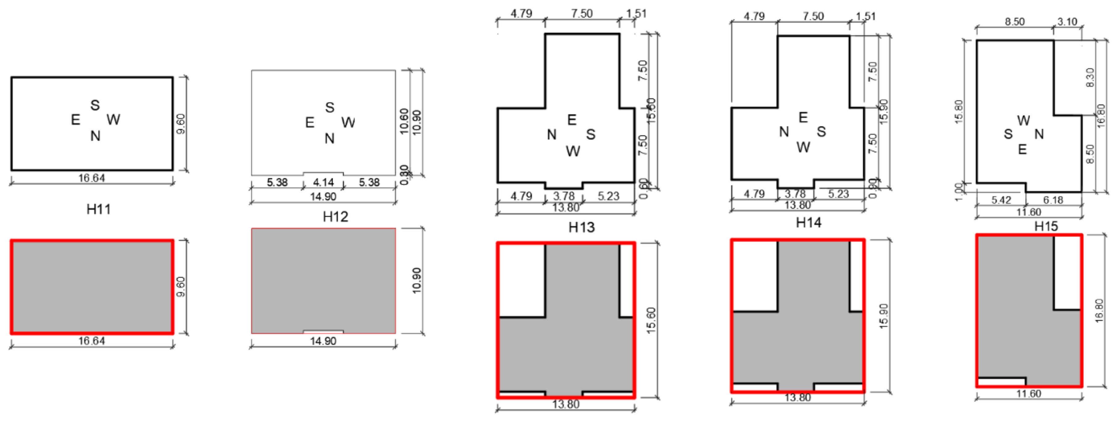
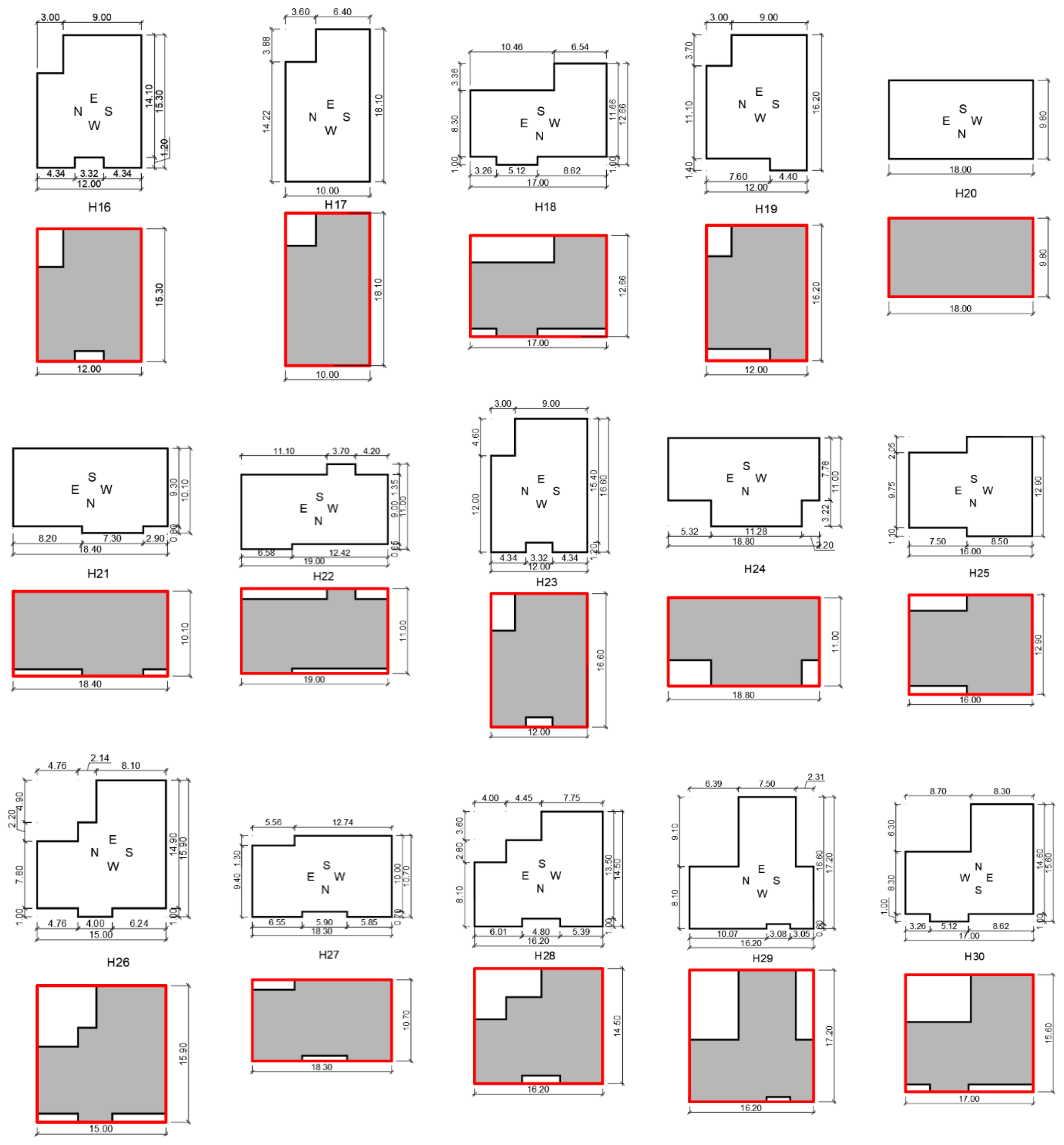
2.1. Selection of a Group of Buildings for Analysis

The present article deals with single-family houses, as these constitute a significant share in all residential buildings. In 2019, more than one third (34.8%) of the EU population lived in detached houses, almost one fifth (18.5%) lived in semi-detached or terraced houses, and 46.1% lived in flats [24]. In Poland, in 2020, single-family buildings constituted 96.8% of all completed residential buildings [25]. Most of the new residential buildings were built using traditional methods [25], and were equipped with a gas boiler for heating [25]. The average usable floor area of houses in Poland was 134.4 m2 [26].
An additional argument for conducting the analysis on this group of buildings is the possibility of erecting small single-family buildings without the need to obtain a building permit, enforced in Polish law from January 2022 [27]. Such buildings should be one-story, without a basement, and with an unoccupied attic.
To carry out the analysis, it was decided that the houses will be located in the city of Białystok in northeastern Poland, i.e., under the conditions of a temperate continental climate according to the Köppen–Geiger climate classification system [28]. The geographic coordinates of the selected city are longitude 23.17° and latitude 53.1°.

2.2. Definitions of Geometric Indicators and Research Hypoteses

In a previous article [7], definitions of indicators were provided. Assuming that Af is the area of the plan of a house, P is the perimeter of the plan of a house, and h is the height of the external wall:
EWA / FA = Ph A f ,
then expressing the ratio of external wall area to floor area;
RC cd = 2 A f + Ph 2 A f + 4 A f h ,
which is the relative compactness indicator with respect to a cuboid;
A / V = Ph + 2 A f A f · h ,
and, finally, expressing the quotient of the total area (in terms of external walls) and the volume of the solid building.
The commonly used A/V ratio has the disadvantage that it is not a dimensionless quantity, and depends on the measurement unit adopted. It turns out that at a constant height h of a building, we have a direct linear relationship between A/V and EWA/FA. Namely, from Equation (3), we have a simple relationship:
A / V = P A f + 2 h .
However, from Equation (1) it can be seen that EWA/FA is a function of the quotient P A f , such that:
EWA / FA = P A f · h ,
Finally, with constant h, a linear relationship is obtained:
A / V = 1 h · ( EWA / FA ) + 2 h .
The indicators (1) and (3) are linearly dependent. Assuming that we are considering buildings with a constant base area Af, a linear relationship between EWA/FA and RCcd is obtained, namely:
RC cd = 2 A f 2 A f + 4 h + A f 2 A f + 4 h E W A / F A ,
Consequently, from Equations (6) and (7), we can determine the dependency between RCcd and A/V:
RC cd = A f · h 2 A f + 4 h A / V ,
and from this, we make the following hypotheses:
Hypothesis 1 (H1). 
Between the geometrical indicators EWA/FA, A/V, and RCcd, the definitions of which are given above, and the demand for useful energy (HOI—indicator of annual demand for utility energy for heating, and OEI—indicator of annual demand for utility energy, taking into account not only heating, but also the preparation of domestic hot water), and finally, HFI (indicator of the annual demand for final energy for heating) and FEI (indicator of the annual demand for final energy, taking into account not only heating, but also the preparation of domestic hot water and the operation of electrical devices) of a single-family house, there is a significant correlation.
Hypothesis 2 (H2).
Assuming that the built-up (building base) areas of single-family houses are equal (in practice: similar), the indicators (RCcd and HOI, RCcd and OEI, RCcd and HFI, RCcd and FEI) are strongly correlated.

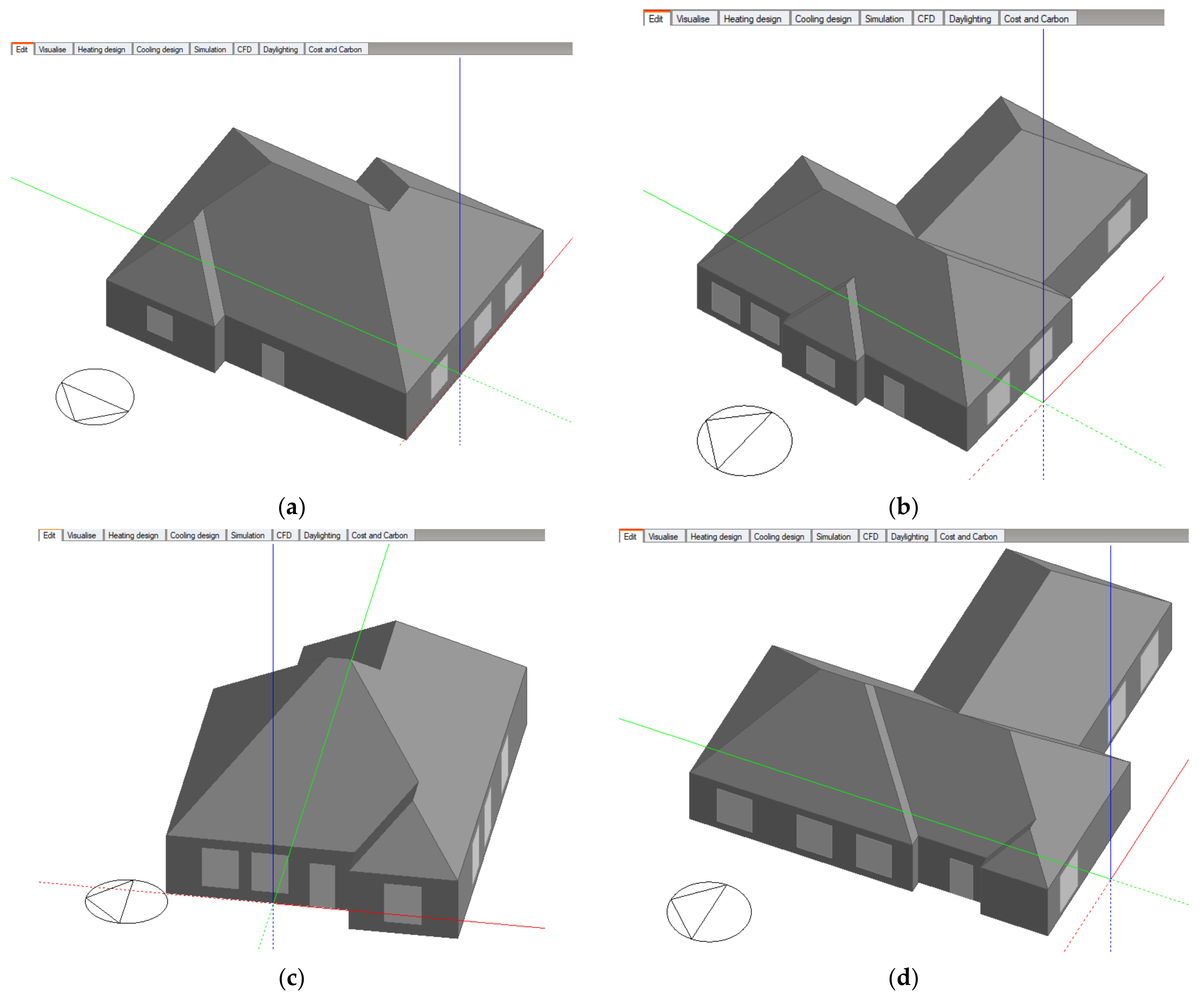
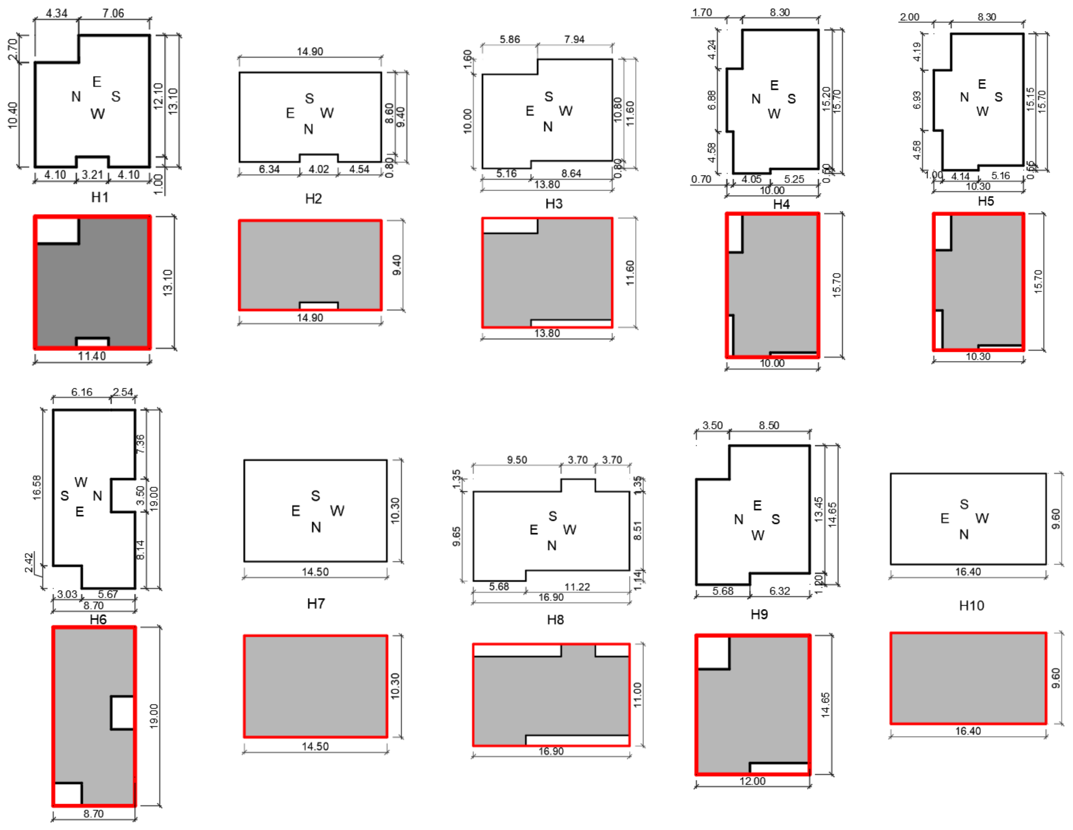
2.3. Selected Designs of Single-Family Houses—The General Characteristics

In this article, we discuss the design class of 30 single-family houses. These are single-story, detached houses with a multi-slope roof, and with a range of 112–170 m2 of usable area.
Schematic plans of the buildings with cardinal directions are shown in Figure A1 and Figure A2 of the Appendix A. We have marked the collection of 30 single-family houses as H1, H2, …, H30; similar to [7], in which these projects were used for analysis in terms of construction costs. Basic geometrical parameters (usable heated area Ah, shape factors A/V and EWA/FA, as well as compactness indicator RCcd) of the analyzed buildings are presented in Table 1a,b.
The present article assumes that parameters related to materials, construction solutions, thickness of insulation layers, etc., are the same for all tested buildings, and typical for current Polish conditions. The thermal properties of materials of the building components are provided in Table 2.
The types of materials listed in Table 2 and their thicknesses were adopted based on catalog projects. Thermal transmittance coefficients of the building envelope were the following: external walls, 0.162 W/(m2·K); celling under an unoccupied attic, 0.143 W/(m2·K); pitched roof under over unoccupied attic, 0.195 W/(m2·K); floor on the ground, 0.243 W/(m2·K). The values of this coefficient met the current requirements for new buildings in Poland [29]. In the case of the ceiling under the unheated attic, the thermal transmittance coefficients turned out to be 5% lower than the maximum permissible value, and in the cases of the external walls and the floor on the ground, this difference was almost 20%.
In addition, painted wooden windows with the coefficients 0.474 (solar heat gain coefficient) and 0.661 (radiation transmittance coefficient) were adopted. Thermal transmittance coefficients were as follows: glass, 0.780 W/(m2·K); frames, 0.881 W/(m2·K); external door, 1.157 W/(m2·K).
The linear thermal transmittances of the thermal bridges, modeled using THERM 6.3 software [30], were the following: roof–wall junction Ψ = 0.017 W/(m∙K); wall–ground floor junctions Ψ = 0.048 W/(m∙K); wall–wall (corner) Ψ = −0.076 W/(m∙K); and wall–window junction Ψ = 0.025 W/(m∙K).
It was assumed, in accordance with the catalog projects, that the buildings had a natural ventilation system, similar to the majority of currently constructed single-family houses in Poland.

2.4. Detailed Assumptions Regarding the Glazing Size in Analyzed Buildings

We conducted our research study on the same H1–H30 buildings (Figure A1 and Figure A2), the catalog designs of which were analyzed in [7], but in a different aspect. In order to achieve the aim set in this article, we made a few additional restrictions, which later allowed us to objectively compare the energy demand of 30 objects in light of changes in their geometric features.
According to Pacheto et al., among the parameters of residential buildings, shape, glazing, and orientation have the greatest impact on reducing energy demand [31]. Goia investigated the optimal window-to-wall ratio (WWR) in office buildings, and its impact on energy savings [32]. Therefore, in order to reliably compare buildings of different shapes, one should pay attention to the relationship between the building’s glazing (the amount of glazing per façade) and its geographical orientation.
In order to assure the homogeneity of the building’s glazing system, we assumed that the ratio of the glazing area to the floor area (referred to in this paper as building area) is constant, and amounts to 0.15 (the minimum in Polish standards is 1/8, i.e., 0.125). According to the actual design assumptions of the H1–H30 buildings, this coefficient is between 0.18 (project H17) and 0.33 (project H17), and on average amounts to 0.25.
We designed the location in such a way that most of the glazed area is on the S side, on average, on the E and W sides, and the least of it on the N side. In particular, we assumed that:
  • The window-to-wall ratio is constant for a given façade in all buildings in the collection H1–H30;
  • Specific window-to-wall ratios are assigned to the different directions of a compass: E—22%, S—40%, W—30%, N—8%;
  • There is a constant ratio of the height (hw) to the width (w) of the window;
  • The windows are single-leaf, three in all directions except the northern N, where we have provided one window.
The calculated glazing areas for the considered buildings are presented in Table 3, where Aw represents the window opening area of the building in a given façade (E, S, W, N).
Assuming the value of k is:
k = h w w ,
where hw is window height, w is window width, and n is the number of windows. With k set to 1.2, the window dimensions hw and w are obtained from the following system of equations:
hw = k·w,
n·w·hw = Aw,
Substituting for hw from Equation (9) into Equation (10) we get:
n·k·w2 = Aw,
and subsequently determine the value of w, as follows:
w = A w n · k .
Applying k = 1.2, n = 3 for the E, S, W directions, and n = 1 for the N direction, following the Equations (9)–(12), we obtain the dimensions of windows at particular elevations (Table 4).
After the window dimensions were unified in the analyzed catalog building designs, models of all buildings were made using DesignBuilder (version 6.1.7.007), developed by the DesignBuilder Software in Stroud, Gloucestershire, UK. [33]. The visualization of four exemplary buildings is shown in Figure 1.
For the calculations, we assumed that buildings had a roof and a base adjusted to the outline (four- or multi-slope).

2.5. Methodology for Calculating Energy Demand, Program Validation, and Calculation Assumptions

The DesignBuilder program [33] version 6.1.7.007 was also utilized to perform the energy simulations. It is based on a calculation engine EnergyPlus. When dealing with buildings at the design stage, it is not recommended, or even possible, to perform real life interventions for research purposes; therefore, only numerical simulations were used in this study to examine the influence of geometrical parameters on energy demand. DesignBuilder has been validated in various studies [34,35,36,37,38] and, additionally, was approved by LEED and meets the Performance Rating Method requirements of the ASHRAE standards [39]. The validation of the simulation results produced with DesignBuilder software in terms of annual energy consumption showed very low levels of error: up to 1.6% [34] or 3.17% [39].
The basis of the method adopted for the determination of heat and mass transport is the formulation of energy and moisture balances in a separate zone of the building, and solving the obtained ordinary differential equations. Heat transport through building partitions is calculated based on the CTF (Conduction Transfer Function). Heat gains from solar radiation through glazed partitions are determined taking into account direct, diffuse, and reflected solar radiation.
We provide the calculation scheme of EnergyPlus™ version 9.3.0 documentation, the basis of which is the differential equation [40]:
C z d T z d t = i = 1 N s l Q ˙ i + i = 1 N s u r f a c e s h i A i ( T s i T z ) + i = 1 N z o n e s m ˙ i C p ( T z i T z ) + m ˙ inf C p T T z + Q ˙ s y s
the parameters of this equation are as follows:
  • i = 1 N s l Q ˙ i = totalized loads of internal convection;
  • i = 1 N s u r f a c e s h i A i (TsiTz) = convective heat dissipation from the zone surfaces;
  • i = 1 N z o n e s m ˙ i C p (TziTz) = heat exchange as a result of inter-zone air mixing;
  • m ˙ inf C p (TTz) = heat exchange as a result of infiltration of external air;
  • Q ˙ s y s = output of air systems;
  • C z d T z d t = energy hidden in the air zone;
  • Cz = ρ a i r C p C T ;
  • ρ a i r = density of zone air;
  • Cp = specific heat of zone air;
  • CT = multiplier of sensible heat capacity [40].
In the calculations, we did not divide the building into rooms, as this would be an additional differentiation between the buildings, and would disturb the homogeneity of the examined objects. We were only interested in differentiating the shape of the building enclosure. We therefore divided the building simply into the ground floor (heated) and the unheated attic. We adopted the hourly balance methods in the calculations. Standard annual meteorological data for Bialystok (Poland) station. We used the search function ‘Weather Data by Location’ [41] in EnergyPlus.
The following assumptions were made for the calculations: the temperature during the heating season is 20 °C, natural ventilation (air exchange) was determined at 0.5 ac/h, all parameters and usage profiles of the building are constant, and only the shape of the building changes.
Occupancy schedules and heat loads in accordance with NCM (National Calculation Method) were applied.
Other assumptions for the calculations include:
  • The average efficiency of the heating system is 0.77 (as a heat source, a gas condensing boiler, and a plate radiator system);
  • There is no building cooling system;
  • The consumption rate of domestic hot water is 1.4 L/(m2day), mains supply temperature is 10 °C, delivery temperature is 55 °C;
  • The average efficiency of the hot water preparation system is 0.43.

3. Results and Discussion

As a result of the calculations (simulations) carried out (using the DesignBuilder program), we obtained the usable and final energy values for individual buildings (Table 5).

3.1. Analysis of Energy Indicators

The HOI energy indices obtained as a result of the simulation, which mainly depends on the thermal quality of the building envelope, the ventilation system, and climatic conditions, ranged from 51.59 kWh/(m2 year) to 56.85 kWh/(m2 year). There are no requirements for an HOI indicator in Polish law. Comparing the obtained results for the group of buildings analyzed in this article with other simulation results for conventional single-family houses (with natural ventilation systems) located in conditions of moderate continental climate [42], similar results were obtained. The thermal quality of the analyzed buildings, expressed by the HOI indicator, was also compared with the levels of indexes required by the Polish energy-saving NF40, NF15 standards [43] and passive standard [44]. The analyzed buildings turned out to be 29–42% worse than the NF40 standard, and more than two times worse than the NF15 and passive standards.
The obtained HFI indicators, referring to the amount of energy supplied to the building as electricity or heat, or as fuel processed for the needs of heating installations (in this case gas), ranged from 67.00 kWh/(m2 year) to 73.83 kWh/(m2 year). The amount of final energy is higher than the amount of usable energy, which results from the energy losses of the building on the way from the place of energy supply to the place of its use (losses related to the efficiency of production systems, transmission, storage, and use of heat). However, these values of final energy are important as they determine the cost of heating and are responsible for pollutant emissions related to heating buildings.

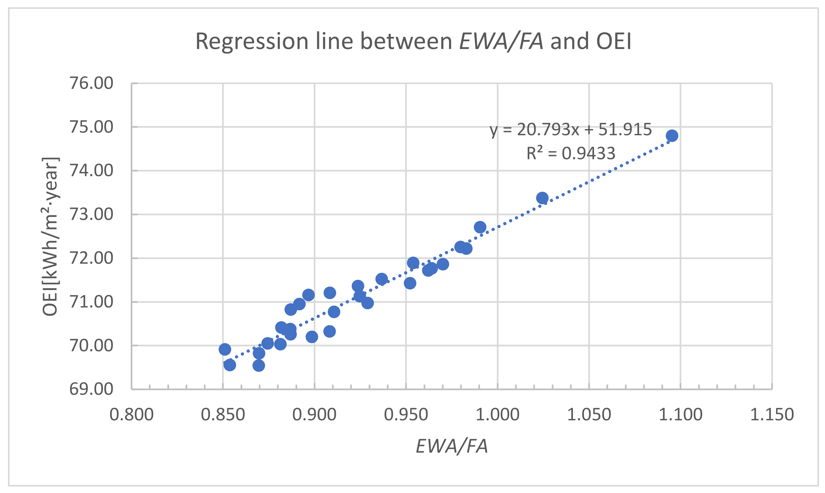
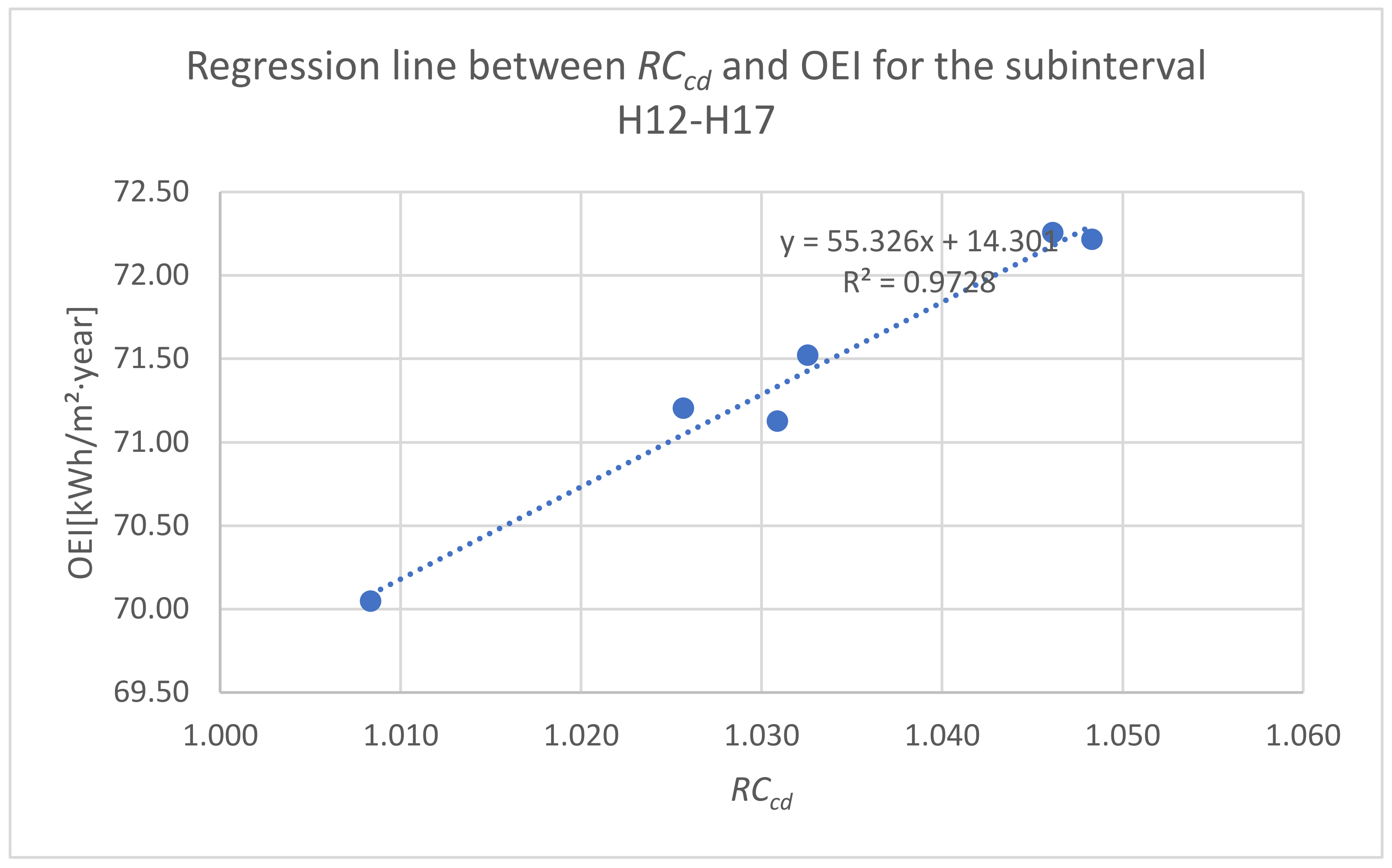
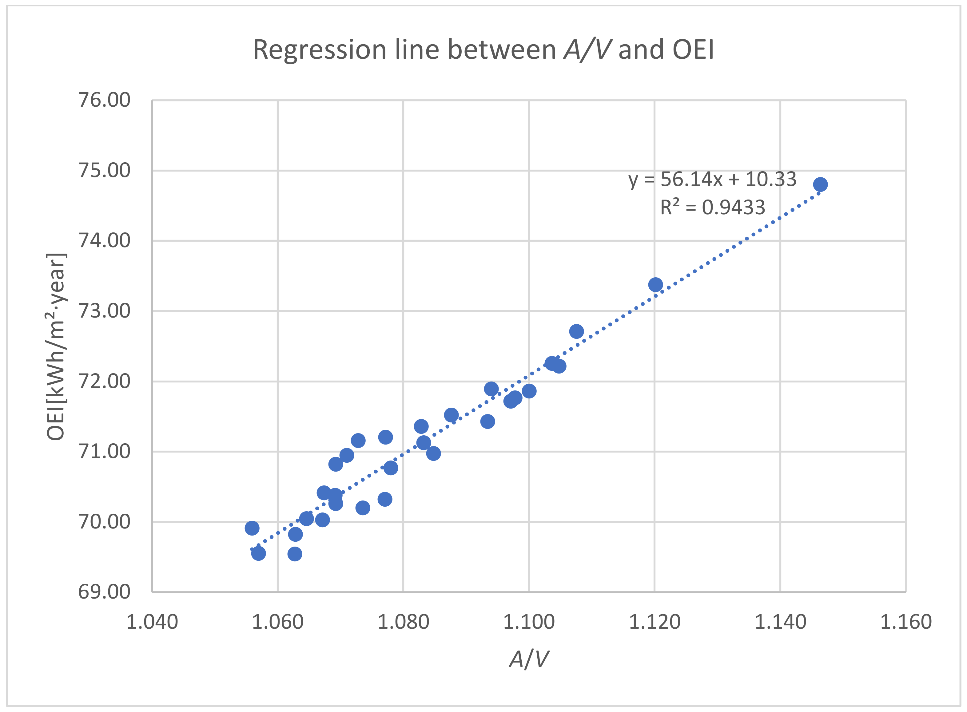
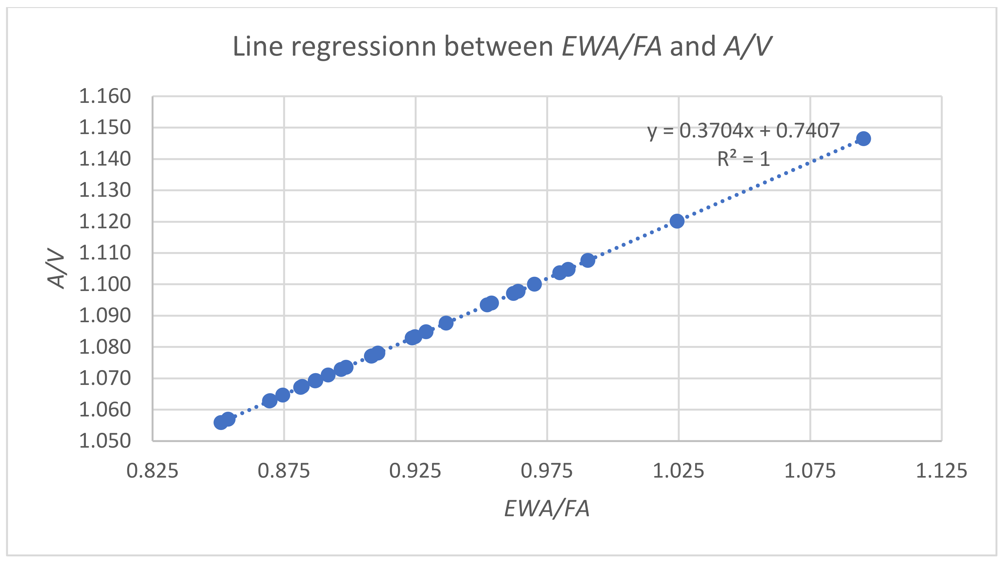
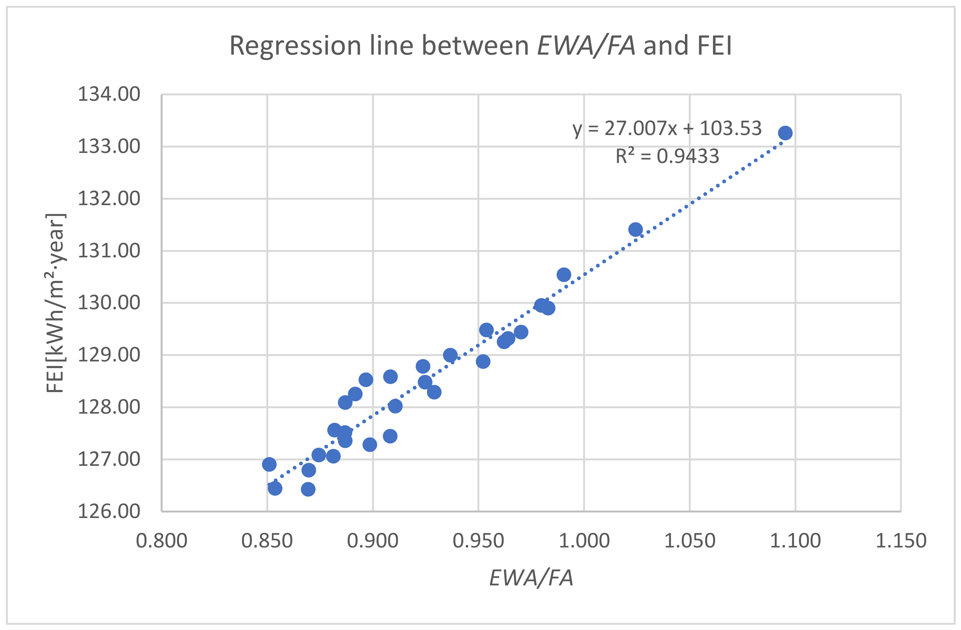
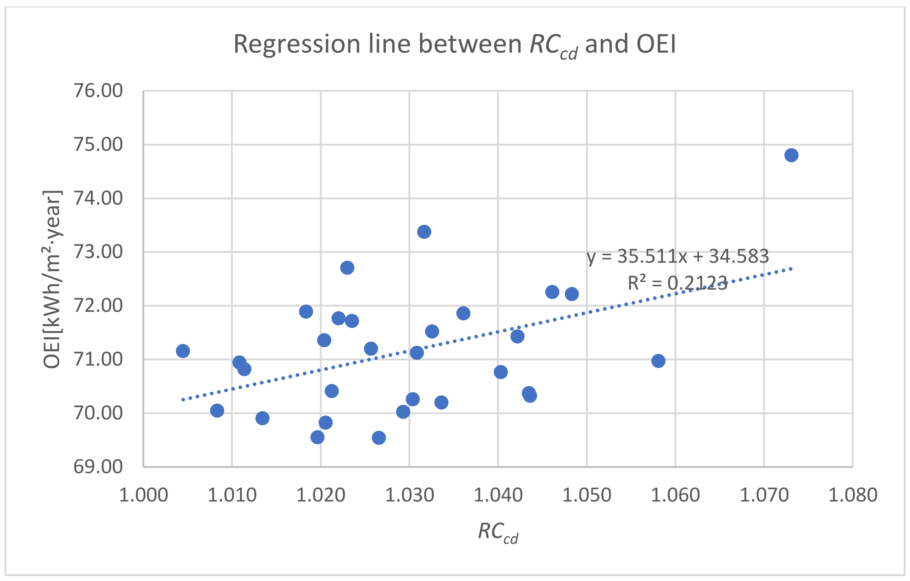
3.2. Analysis of the Dependence of Indicators

We will now discuss the results. The research hypothesis based on the supposition that there are strong linear dependencies between the values of the parameters EWA/FA and OEI, A/V, and OEI, and similarly between EWA/FA and FEI, and A/V and FEI. For this purpose, we performed a regression analysis. Selected results of the analysis are presented in charts (Figure 2, Figure 3, Figure 4, Figure 5, Figure 6 and Figure 7). Indeed, strong linear relationships confirm the research hypothesis that by reducing the EWA/FA parameter, we reduce the size of OEI energy demand (Figure 2). Similarly, a reduction in the OEI size was obtained as a result of the reduction in the A/V parameter (Figure 3); this is not surprising, because with the adopted assumption h = const, we proved a direct mathematical relationship (6). The confirmation of this fact was also obtained as a result of our calculations, where the coefficient of determination R2 = 1 (Figure 4).
The calculation results obtained with DesignBuilder in relation to the fit of the regression lines for EWA/FA and A/V to the final energy demand of FEI are almost identical. The determination coefficient R2 even turned out to be the same (Figure 5). For obvious reasons, due to the nature of the concepts of operational energy and final energy, the OEI and FEI values are respectively different (Table 5). As we have already said, the EWA/FA and A/V parameters have the disadvantage that their values for the reference building, which is a square with a square base (square with side a) and height h, are, respectively, 4 h a , and 4 a + 2 h , and depend on the value of a. Thus, it is not possible to unequivocally establish a meaningful comparative threshold. The relative compactness index RCcd does not have this disadvantage. Its value for the reference solid is 1, while the value for any prism other than a cuboid is greater than 1. The indicator has another disadvantage, namely, it depends on the base area (building development area). Hence, in the discussed case study of 30 single-family houses with highly dispersed building area values, ranging from 134.41 m2 to 198.51 m2, we observed no correlation between RCcd and OEI, with R2 = 0.2123 (row 1 in Table 1 and row 8 in Table 5; Figure 6). However, the relationship between RCcd and OEI (R2 = 0.9728) appears relatively strong for buildings with a small spread of the built-up area, ranging from 161.17 m2 to 167.03 m2 (line 1 in Table 1 and line 8 in Table 5; Figure 7).
For example, let us assume that the building base area is fixed. In practice, this means that the architect intends to design a house with a predetermined building base area. Thus, the variants of the base polygon shape analyzed by the architect always have an area close to a predetermined size, e.g., 125 m2. As such, according to Equations (7) and (8), and the commentary following these formulas, the relative compactness index RCcd measures the OEI and FEI values very well. Figure 6 is a very good illustration of this measure, despite the relatively large span of the areas. (167.03 m2 − 161.17 m2 = 5.86 m2).
The low correlation coefficient between the indicators in the interval with too large a span (Figure 6), and the high correlation coefficient in the interval with a short span (Figure 7) provide a good explanation for the lack of correlation in paper [22] between the values of geometric indicators and the energy consumption of buildings. This means that the study of randomly selected buildings, where the range of various parameters is quite large, is doomed to failure. Therefore, in this study, the unification of many parameters was adopted to test only a select few.
Among the analyzed parameters EWA/FA, A/V, and RCcd, the RCcd index is the best measure of energy demand because it has a direct reference to the reference solid, which is a cuboid. Moreover, the RCcd index with values greater than or equal to one simply reflects the deviation of the shape of a building from the optimal value, which is 1. This deviation can be easily expressed in percentage points by multiplying the obtained value by 100. This gives the designer the ability to easily evaluate the adopted design concept in terms of energy demand.
The compliance of the discussed parameters with the energy demand is even easier to obtain if we use the correlation coefficient for the comparison. The indicators describing energy demand for the studied buildings, determined with the use of the DesignBuilder program (EnergyPlus), have now been compared with the shape indicators (EWA/FA and A/V) using the concept of correlation. We have included the results in Table 6. As you can see, the correlations 1 and 5; 2 and 6; 3 and 7; and 4 and 8 are identical. This is (of course) due to the fact that the EWA/FA and A/V parameters are linearly dependent (see (6), Figure 3). This proves the strong correlation of these indicators (see Figure 1, Figure 2, Figure 3 and Figure 4 and Table 7), which in turn proves the correctness of hypothesis 1.
According to Formula (8), assuming that h = const, we obtain identical relationships for cor(A/V, HOI), cor(A/V, OEI), cor(A/V, HFI), and cor(A/V, FEI).
This is an unexpected result, as the A/V (m−1) ratio, which depends on the adopted measurement units, so far considered imperfect, in this case fulfills its function well.
The disadvantage of the A/V ratio is still the lack of a natural, readable reference value.
The Af values (built-up areas) of buildings H12–H17 are close to each other, hence the correlations in the second column of Table 6 are high. This proves the strong correlation of these indicators (Figure 6 and Table 6), which in turn proves the correctness of Hypothesis 2.
Assuming that A = const (this is the case when the architect is looking for the shape of a building with a predetermined building area), on the basis of (12), the effective use of the indicator A/V is possible only with the natural RCcd indicator. The natural reference value of the RCcd indicator is 1.
Referring again to article [22], in the context of the research carried out in this paper, we believe that the impact of each indicator on energy demand should be analyzed while treating the others as constant. Then the test results will be more reliable.
An ideal confirmation of the research carried out in the present study would be to examine the actual energy consumption in several dozen built, inhabited, and operated buildings that are properly designed (the same building base area, different shapes of the building contour, the same materials and technologies used in the construction). This is an interesting problem to be solved in the future.

4. Conclusions

The present article contains research, unprecedented in the literature, carried out on a set of real life single-family house designs, slightly modified in terms of the conducted research. Therefore, our results should be considered extremely reliable. Assuming a constant building area and building height, linear relationships between the indicators EWA/FA and A/V and between RCcd and EWA/FA were derived. These results have interesting consequences in terms of the energy demand of a single-family house.
The geometric form of the house, expressed by the building compactness indicators presented in this paper, has an essential impact on the energy demand. The strong correlation between EWA/FA and A/V indicators and energy demand, obtained on the basis of the collection of actual construction projects, allows one to predict energy demand at the first stage of design.
RCcd is the best measure of energy demand because it has a direct reference to a cuboid building shape, and its value simply reflects the deviation of the building shape from the optimal value, which is 1. This deviation can be easily expressed in percentage points, which makes it easier for the designer to make a decision regarding the project concept in terms of energy demand.
The proposed system of EWA/FA, A/V, and RCcd indicators will be useful for the designer while optimizing the geometric form of a single-family house in terms of reducing energy demand. During the initial shaping of the building form with the assumed building area, the architect should choose the version of the RCcd indicator with the lowest value from among many attempts.
It is worth including the proposed system of EWA/FA, A/V, and RCcd indicators in the BIM description of the building. It is, in a way, a geometric building code, important in an operational aspect.
In fact, among the existing single-family houses, it is difficult to find buildings with the same built-up area, built with the same technology, located in the same climatic zone, with the same WWR ratio, etc. However, it would be valuable to confirm the results of the research presented in this paper with reference to real life single-family houses. This work is an excellent methodological study for conducting such research.

Author Contributions

E.K. has developed the first conceptualization and methodology, prepared and wrote Section 2.2, Section 2.4 and Section 3.2, prepared Table 3a,b, Table 4a,b and Table 6; E.K. and B.S. prepared introduction and Section 2.1, discussed and perfected the detailed methodology, literature study; K.B. prepared preliminary data, Figure A1 and Figure A2 and Table 1a,b; B.S. performed calculations in the DesignBuilder software and prepared the Section 2.3, Section 2.5 and Section 3.1, Table 2 and Figure 1; E.K. and B.S., conducted the analysis, made their final conclusions and wrote the manuscript; E.K., B.S. and K.B. have read and agreed to the published version of the manuscript. All authors have read and agreed to the published version of the manuscript.

Funding

This work was performed within the framework of grants of the Bialystok University of Technology (WZ/WBiNS/4/2022, WZ/WBiNS/3/2022) and financed by the Ministry of Science and Higher Education of the Republic of Poland.

Institutional Review Board Statement

Not applicable.

Informed Consent Statement

Not applicable.

Data Availability Statement

Not applicable.

Conflicts of Interest

The authors declare no conflict of interest. The funders had no role in the design of the study; in the collection, analyses, or interpretation of data; in the writing of the manuscript; or in the decision to publish the results.

Symbols and Abbreviations

SymbolAbbreviationUnit
Ahusable heated area of buildingm2
Afbase area of buildingm2
Pperimeter of the plan of buildingm
hheight of external wallm
Atotal area of buildingm2
Awwindow opening aream2
hwwindow heightm
wwindow widthm
kthe ratio of hw and w-
nnumber of windows-
c z heat capacity of the zoneJ/K
T z zone air temperature°C
ttimes
Nlnumber of internal loads-
Q i ˙ internal loadW
Nsnumber of zone surfaces-
hiconvective heat transfer coefficientW/(m2·K)
Aiarea of zone surfacem2
Tsitemperature of zone surface°C
m ˙ i inter-zone mass flow ratekg/s
cpair specific heatJ/(kg·K)
Tsitemperature of zone surface°C
Nznumber of adjacent zones-
Tzitemperature of adjacent zone°C
m ˙ i n f infiltration mass flow ratekg/s
Tambambient air temperature°C
m ˙ s y s HVAC system mass flow ratekg/s
Tssupply air temperature°C

Appendix A

Figure A1. Building plans of the H1–H15 collection with cardinal directions.
Energies 15 03308 g0a1aEnergies 15 03308 g0a1b
Figure A2. Building plans of the H16–H30 collection with cardinal directions.
Energies 15 03308 g0a2

References

  1. Tsemekidi Tzeiranaki, S.; Bertoldi, P.; Diluiso, F.; Castellazzi, L.; Economidou, M.; Labanca, N.; Ribeiro Serrenho, T.; Zangheri, P. Analysis of the EU Residential Energy Consumption: Trends and Determinants. Energies 2019, 12, 1065. [Google Scholar] [CrossRef] [Green Version]
  2. Coma, J.; Maldonado, J.M.; de Gracia, A.; Gimbernat, T.; Botargues, T.; Cabeza, L.F. Comparative Analysis of Energy Demand and CO2 Emissions on Different Typologies of Residential Buildings in Europe. Energies 2019, 12, 2436. [Google Scholar] [CrossRef] [Green Version]
  3. National Plan for Increasing the Number of Nearly Zero-Energy Buildings as Required by Directive 2010/31/EU on the Energy Performance of Buildings (EPBD recast)—Poland. J. Law Rep. Pol. 2015, Item 614. (In Polish)
  4. Statistics Poland. Household Energy Consumption in 2018, Warsaw, Poland. 2019. Available online: https://stat.gov.pl/obszary-tematyczne/srodowisko-energia/energia/zuzycie-energii-w-gospodarstwach-domowych-w-2018-roku,2,4.html (accessed on 20 May 2020).
  5. BPIE; Staniaszek, D.; Firląg, S.Z. Financing Building Energy Performance Improvement in Poland. Status Report. 2016. Available online: http://bpie.eu/publication/financing-building-energy-performance-improvement-in-poland-status-report/ (accessed on 20 May 2020).
  6. Chen, S.; Zhang, G.; Xia, X.; Setunge, S.; Shi, L. A review of internal and external influencing factors on energy efficiency design of buildings. Energy Build. 2020, 216, 109944. [Google Scholar] [CrossRef]
  7. Koźniewski, E.; Banaszak, K. Geometric Aspects of Assessing the Amount of Material Consumption in the Construction of a Designed Single-Family House. Energies 2020, 13, 5382. [Google Scholar] [CrossRef]
  8. D’Amico, B.; Pmponi, F. A Compactness Measure of Sustainable Building Forms. R. Soc. Open. Sci. 2019, 6, 181265. [Google Scholar] [CrossRef] [Green Version]
  9. Yoshino, H.; Hong, T.; Nord, N. IEA EBC annex 53: Total energy use in buildings—Analysis and evaluation methods. Energy Build. 2017, 152, 124–136. [Google Scholar] [CrossRef] [Green Version]
  10. Obrecht, T.; Vesn, M.P.; Leskovar, Ž. Influence of the orientation on the optimal glazing size for passive houses in different European climates (for non-cardinal directions). Sol. Energy 2019, 189, 15–25. [Google Scholar] [CrossRef]
  11. Hong, T.; Taylor-Lange, S.C.; D’Oca, S.; Yan, D.; Corgnati, S.P. Advances in research and applications of energy-related occupant behavior in buildings 2016. Energy Build. 2016, 116, 694–702. [Google Scholar] [CrossRef] [Green Version]
  12. Tukhtamisheva, A.; Adilova, D.; Banionis, K.; Levinskytė, A.; Bliūdžius, R. Optimization of the Thermal Insulation Level of Residential Buildings in the Almaty Region of Kazakhstan. Energies 2020, 13, 4692. [Google Scholar] [CrossRef]
  13. Kormaníková, L.; Kormaníková, E.; Katunský, D. Shape Design and Analysis of Adaptive Structures. Procedia Eng. 2017, 190, 7–14. [Google Scholar] [CrossRef]
  14. Chwieduk, D.; Chwieduk, M. Determination of the Energy Performance of a Solar Low Energy House with Regard to Aspects of Energy Efficiency and Smartness of the House. Energies 2020, 13, 3232. [Google Scholar] [CrossRef]
  15. Allouhi, A.; El Fouih, Y.; Kousksou, T.; Jamil, A.; Zeraouli, Y.; Mourad, Y. Energy consumption and efficiency in buildings: Current status and future trends. J. Clean. Prod. 2015, 109, 118–130. [Google Scholar] [CrossRef]
  16. Depecker, P.; Menezo, C.; Virgone, J.; Lepers, S. Design of buildings shape and energetic consumption. Build. Environ. 2001, 36, 627–635. [Google Scholar] [CrossRef]
  17. Jedrzejuk, H.; Marks, W. Optimization of shape and functional structure of buildings as well as heat source utilisation. Partial problem solution. Build. Environ. 2002, 37, 1037–1043. [Google Scholar] [CrossRef]
  18. Parasonic, J.; Keizikas, A.; Endriukaitytė, A.; Kalibatienė, D. Architectural Solutions to Increase the Energy Efficiency of Buildings. J. Civ. Eng. Manag. 2012, 18, 71–80. [Google Scholar] [CrossRef]
  19. Pessenlehner, W.; Mahdavi, A. Building Morphology, Transparence, and Energy Performance. In Proceedings of the 8th International IBPSA Conference, Eindhoven, The Netherlands, 11–14 August 2003; pp. 1025–1032. [Google Scholar]
  20. Ourghi, R.; Al-Anzi, A.; Krarti, M. A simplified analysis method to predict the impact of shape on annual energy use for office buildings. Energy Convers. Manag. 2007, 48, 300–305. [Google Scholar] [CrossRef]
  21. McKeen, P.; Fung, A.S. The Effect of Building Aspect Ratio on Energy Efficiency: A Case Study for Multi-Unit Residential Buildings in Canada. Buildings 2014, 4, 336–354. [Google Scholar] [CrossRef]
  22. Rodrigues, E.; Amaral, A.R.; Gaspar, A.R.; Gomes, A. How reliable are geometry-based building indices as thermal performance indicators? Energy Convers. Manag. 2015, 101, 561–578. [Google Scholar] [CrossRef]
  23. Koźniewski, E.; Żaba, A.; Dudzik, P. The Compactness Indicators of Solids Applied to Analysis of Geometric Efficiency of Buildings. J. Civ. Eng. Manag. 2019, 25, 742–756. [Google Scholar] [CrossRef] [Green Version]
  24. Eurostat—Statistic Explained. Living Conditions in Europe—Housing. 2021. Available online: https://ec.europa.eu/eurostat/statistics-explained/index.php?title=Living_conditions_in_Europe_-_housing (accessed on 10 March 2022).
  25. Statistics Poland. Statistical Analyses. Construction Result in 2020; Statistical Office in Lublin: Lublin, Poland, 2021; p. 18.
  26. Report on the Construction of Houses in Poland in 2018. Available online: https://www.nieruchomosci.egospodarka.pl/154042,Budowa-domow-w-Polsce-2018,1,80,1.html (accessed on 10 March 2022).
  27. Legal Act of the Sejm of the Republic of Poland of 17 September 2021 amending the Act—Building Law and the Act on Spatial Planning and Development. Journal of Laws of 2021, item 1986.
  28. Peel, M.C.; Finlayson, B.L.; McMahon, T.A. Updated world map of the Köppen-Geiger climate classification. Hydrol. Earth Syst. Sci. 2007, 11, 1633–1644. [Google Scholar] [CrossRef] [Green Version]
  29. Polish Ministry of Transport, Construction and Maritime Economy. Regulation of the Minister of Transport, Construction and Maritime Economy of 5 July 2013 on the Technical Conditions that Buildings and Their Location Should Satisfy; Polish Ministry of Transport, Construction and Maritime Economy: Warsaw, Poland, 2015.
  30. Software Informer Home Page. The THERM 6.3 Software, the Lawrence Berkeley National Laboratory (LBNL) Berkeley, USA. Available online: https://therm.software.informer.com/ (accessed on 1 April 2021).
  31. Pacheco, R.; Ordonez, J.; Martinez, G. Energy efficient design of building: A review. Renew. Sustain. Energy Rev. 2012, 16, 3559–3573. [Google Scholar] [CrossRef]
  32. Goia, F. Search for the optimal window-to-wall ratio in office buildings in different European climates and the implications on total energy saving potential. Sol. Energy 2016, 132, 467–492. [Google Scholar] [CrossRef]
  33. Software Informer Home Page. DesignBuilder Software—Private Limited Company No. 04514127; DESIGNBUILDER SOFTWARE LIMITED, Stroud House, Stroud, Loucestershire, UK. Available online: https://designbuilder.co.uk/download/previous-versions (accessed on 1 April 2021).
  34. Fathalian, A.; Kargarsharifabad, H. Actual validation of energy simulation and investigation of energy management strategies (Case Study: An office building in Semnan, Iran). Case Stud. Therm. Eng. 2018, 12, 510–516. [Google Scholar] [CrossRef]
  35. Ismail, A.M.; Abo Elela, M.M.; Ahmed, E.B. Calibration of Design Builder program. J. Am. Sci. 2015, 11, 96–102. [Google Scholar]
  36. Baharvand, M.; Ahmad, M.H.B.; Safikhani, T.; Majid, R.B.A. DesignBuilder verification and validation for indoor natural Ventilation. J. Basic Appl. Sci. Res. 2013, 3, 182–189. [Google Scholar]
  37. Raji, B.; Tenpierik, M.; Bokel, R.; van den Dobbelsteen, A. Natural summer ventilation strategies for energy-saving in high-rise buildings: A case study in The Netherlands. Int. J. Vent. 2019, 19, 25–48. [Google Scholar] [CrossRef] [Green Version]
  38. Roshan, G.; Arab, M.; Klimenko, V. Modeling the impact of climate change on energy consumption and carbon dioxide emissions of buildings in Iran. J. Environ. Health Sci. Eng. 2019, 17, 889–906. [Google Scholar] [CrossRef]
  39. Al-Sakkaf, A.; Mohammed Abdelkader, E.; Mahmoud, S.; Bagchi, A. Studying Energy Performance and Thermal Comfort Conditions in Heritage Buildings: A Case Study of Murabba Palace. Sustainability 2021, 13, 12250. [Google Scholar] [CrossRef]
  40. U.S. Department of Energy. EnergyPlus™ Version 9.3.0 Documentation. Engineering Reference. Build: baff08990c. 2020. Available online: https://www.google.com/url?sa=t&rct=j&q=&esrc=s&source=web&cd=&ved=2ahUKEwi_5aqBpbftAhUllosKHQCPDR0QFjAAegQIBRAC&url=https%3A%2F%2Fenergyplus.net%2Fsites%2Fall%2Fmodules%2Fcustom%2Fnrel_custom%2Fpdfs%2Fpdfs_v9.3.0%2FEngineeringReference.pdf&usg=AOvVaw1drV7NwKPCki4unAIb0UZ6 (accessed on 1 April 2021).
  41. EnergyPlus—Weather Data by Location. Available online: https://energyplus.net/weather-location/europe_wmo_region_6/POL//POL_Bialystok.122950_IMGW (accessed on 1 April 2021).
  42. Sadowska, B. The Impact of Climate Conditions on Energy Consumption for Heating and Cooling of Residential Buildings. Econ. Environ. 2018, 67, 189–197. Available online: https://www.ekonomiaisrodowisko.pl/journal/article/view/128/122 (accessed on 1 April 2022).
  43. National Fund for Environmental Protection and Water Management. Priority Program—Effective Use of Energy. Subsidies for Loans for the Construction of Energy-Efficient Houses. Available online: http://oze.nfosigw.gov.pl/oferta-finansowania/srodki-krajowe/programy-priorytetowe/doplaty-do--kredytow-na-domy-energooszczedne/informacje-o-programie/ (accessed on 10 March 2022). (In Polish)
  44. Passipedia—The Passive House Resource. Criteria for the Passive House, EnerPHit and PHI Low Energy Building Standard. Available online: https://passipedia.org/_media/picopen/9f_160815_phi_building_criteria_en.pdf (accessed on 10 March 2022).
Figure 1. Visualization of example buildings: (a) H3; (b) H13; (c) H19; (d) H29.
Energies 15 03308 g001
Figure 2. High degree of regression line fit as an approximation of the linear dependence of the OEI dependent variable on the independent EWA/FA variable.
Energies 15 03308 g002
Figure 3. High degree of regression line fit as an approximation of the linear dependence of the OEI dependent variable on the independent A/V variable.
Energies 15 03308 g003
Figure 4. Perfect fit of the regression line for EWA/FA and A/V parameters as an illustration of their mutual linear relationship (6).
Energies 15 03308 g004
Figure 5. High degree of regression line fit as an approximation of the linear dependence of the FEI dependent variable on the independent EWA/FA variable.
Energies 15 03308 g005
Figure 6. Weak correlation between RCcd and OEI in the case study of 30 single-family houses with highly dispersed building base area values ranging from 134.41 m2 to 198.51 m2.
Energies 15 03308 g006
Figure 7. The relative compactness index RCcd measures the size of OEI very well.
Energies 15 03308 g007
Table 1. (a) Basic geometrical parameters of the buildings H1–H15 [7]. (b) Basic geometrical parameters of the buildings H16–H30 [7].
(a)
ParameterUnitBuilding Number
H1H2H3H4H5H6H7H8H9H10H11H12H13H14H15
Ahm2112.28115.06121.74121.64123.32122.67127.84130.99132.62134.85136.94138.49136.37137.23138.98
A/Vm−11.121.111.091.101.101.151.071.101.081.071.071.061.101.101.09
EWA/FA-1.020.990.950.960.961.100.900.970.920.890.890.870.980.980.94
RCcd-1.0321.0231.0181.0221.0241.0731.0041.0361.0201.0111.0111.0081.0461.0481.033
(b)
ParameterUnitBuilding Number
H16H17H18H19H20H21H22H23H24H25H26H27H28H29H30
Ahm2141.58142.55142.31148.09152.19152.12154.08155.41156.58157.57156.22158.53160.76167.83169.98
A/Vm−11.081.081.091.071.061.061.071.071.071.061.081.061.081.081.07
EWA/FA-0.920.910.950.880.850.870.900.890.880.850.910.870.910.930.89
RCcd-1.0311.0261.0421.0211.0131.0211.0341.0301.0291.0201.0401.0271.0441.0581.043
Table 2. Thermal properties of materials of components in the buildings being studied.
Material LayersThickness (m)Thermal Conductivity (W/m K)Density (kg/m3)
External wallsEPS Expanded polystyrene0.200.0415
Aerated concrete block0.240.24750
Plastering0.010.821680
Celling under an unoccupied atticMineral wool0.240.03699
Reinforced concrete slab0.151.702200
Plastering0.010.821680
Pitched roof—unoccupied atticClay tile—roofing0.0251.002000
Mineral wool0.240.03699
Plasterboard0.0250.252800
Floor on the groundFloor screed0.050.411200
EPS Expanded polystyrene0.150.0415
Cast concrete0.101.132000
Table 3. (a) Determination of the glazing area of the walls of individual façades of buildings H1–H15. (b) Determination of the glazing area of the walls of individual façades of buildings H16–H30.
(a)
Areas [m2]Building Number
H1H2H3H4H5H6H7H8H9H10H11H12H13H14H15
Base area (Af)134.41136.84143.79143.96145.91149.08149.35155.29155.79157.44159.74161.17162.02163.15163.73
Total glazing area
(0.15 Af)
20.1620.5321.5721.5921.8922.3622.4023.2923.3723.6223.9624.1824.3024.4724.56
Window opening area (Aw)
of individual façades
E4.444.524.754.754.824.924.935.125.145.205.275.325.355.385.40
S8.068.218.638.648.758.948.969.329.359.459.589.679.729.799.82
W6.056.166.476.486.576.716.726.997.017.087.197.257.297.347.37
N1.611.641.731.731.751.791.791.861.871.891.921.931.941.961.96
(b)
Areas [m2]Building Number
H16H17H18H19H20H21H22H23H24H25H26H27H28H29H30
Base area (Af)166.42167.03168.19172.66176.40176.96180.27181.42182.59182.78183.22184.45188.48197.62198.51
Total glazing area (0.15 Af)24.9625.0525.2325.9026.4626.5427.0427.2127.3927.4227.4827.6728.2729.6429.78
Window opening area (Aw)
of individual façades
E5.495.515.555.705.825.845.955.996.036.036.056.096.226.526.55
S9.9910.0210.0910.3610.5810.6210.8210.8910.9610.9710.9911.0711.3111.8611.91
W7.497.527.577.777.947.968.118.168.228.238.248.308.488.898.93
N2.002.002.022.072.122.122.162.182.192.192.202.212.262.372.38
Table 4. (a) Dimensions of the windows on the individual façades of buildings H1–H15. (b) Dimensions of the windows on the individual façades of buildings H16–H30.
(a)
Dimension of the Windows of Individual Façades (m)Building Number
H1H2H3H4H5H6H7H8H9H10H11H12H13H14H15
E façadehw1.111.121.151.151.161.171.171.191.201.201.211.221.221.221.23
w1.331.341.381.381.391.401.401.431.431.441.451.461.461.471.47
S façadehw1.501.511.551.551.561.581.581.611.611.621.631.641.641.651.65
w1.801.811.861.861.871.891.891.931.931.941.961.971.971.981.98
W façadehw1.301.311.341.341.351.371.371.391.401.401.411.421.421.431.43
w1.561.571.611.611.621.641.641.671.671.681.701.701.711.711.72
N façadehw1.161.171.201.201.211.221.221.251.251.251.261.271.271.281.28
w1.391.401.441.441.451.471.471.501.501.511.521.521.531.531.54
(b)
Dimension of the Windows of Individual Façades (m)Building Number
H16H17H18H19H20H21H22H23H24H25H26H27H28H29H30
E façadehw1.241.241.241.261.271.271.291.291.291.291.301.301.311.351.35
w1.481.481.491.511.531.531.541.551.551.551.561.561.581.621.62
S façadehw1.671.671.671.701.711.721.731.741.741.751.751.751.771.811.82
w2.002.002.012.042.062.062.082.092.092.092.102.102.132.182.18
W façadehw1.441.441.451.471.481.491.501.511.511.511.511.521.531.571.58
w1.731.731.741.761.781.781.801.811.811.811.821.821.841.891.89
N façadehw1.291.291.301.311.331.331.341.351.351.351.351.361.371.411.41
w1.551.551.561.581.591.601.611.621.621.621.621.631.651.691.69
Table 5. Usable and final energy demand for buildings H1–H15. End use (kWh/year): (1) heating; (2) DHW; (3) sum total (OE), (4) usable heated area Ah (m2); (5) shape factor A/V (m−1); Operational Energy Indicators (utility use per conditioned floor area (kWh/m2·year): (6) heating (gas), EUH (HOI); (7) DHW (gas), EUW; (8) sum total (OEI). Final use (kWh/year): (9) heating (gas); (10) DHW (gas); (11) auxiliary equipment (electricity); (12) room appliances (electricity); (13) sum total (FE) (kWhyear); Final Energy Indicators: (kWh/m2·year): (14) heating (gas) (HFI); (15) DHW (gas); (16) auxiliary equipment (electricity); (17) room appliances (electricity); (18) sum total (FEI); (19) shape factor EWA/FA; (20) compactness indicator RCcd. (a) values for buildings H1–H15 (b) values for buildings H16–H30.
(a)
Building Number
H1H2H3H4H5H6H7H8H9H10H11H12H13H14H15
16223.476300.676567.166546.406630.776974.106802.197062.087083.257146.967240.447215.117405.897447.187445.68
22015.372065.312185.172183.362213.532201.852294.622351.152380.352420.452457.932485.752447.692463.202494.58
38238.848365.988752.338729.768844.309175.959096.819413.239463.609567.419698.379700.869853.589910.389940.26
4112.28115.06121.74121.64123.32122.67127.84130.99132.62134.85136.94138.49136.37137.23138.98
51.121.111.091.101.101.151.071.101.081.071.071.061.101.101.09
655.4354.7653.9453.8253.7756.8553.2153.9153.4153.0052.8752.1054.3154.2753.57
717.9517.9517.9517.9517.9517.9517.9517.9517.9517.9517.9517.9517.9517.9517.95
873.3872.7171.8971.7771.7274.8071.1671.8671.3670.9570.8270.0572.2672.2271.52
98082.438182.698528.788501.828611.399057.278834.019171.539199.039281.779403.179370.279618.049671.669669.71
104686.914803.055081.795077.585147.745120.585336.335467.795535.705628.955716.125780.815692.305728.375801.35
11347.15355.75376.39376.06381.28379.27395.25404.98410.01416.92423.37428.17421.61424.28429.69
121638.321678.891776.351774.881799.401789.911865.331911.281935.051967.611998.082020.691989.762002.372027.87
1314,754.8115,020.3715,763.3115,730.3415,939.8116,347.0316,430.9216,955.5817,079.7817,295.2517,540.7417,599.9517,721.7117,826.6817,928.62
1471.9871.1270.0669.8969.8373.8369.1070.0269.3668.8368.6767.6670.5370.4869.58
1541.7441.7441.7441.7441.7441.7441.7441.7441.7441.7441.7441.7441.7441.7441.74
163.093.093.093.093.093.093.093.093.093.093.093.093.093.093.09
1714.5914.5914.5914.5914.5914.5914.5914.5914.5914.5914.5914.5914.5914.5914.59
18131.41130.54129.48129.32129.26133.26128.53129.44128.79128.26128.09127.08129.95129.90129.00
191.020.990.950.960.961.100.900.970.920.890.890.870.980.980.94
201.0321.0231.0181.0221.0241.0731.0041.0361.0201.0111.0111.0081.0461.0481.033
(b)
Building Number
H16H17H18H19H20H21H22H23H24H25H26H27H28H29H30
17528.967591.507610.677769.717907.927891.238050.628129.738154.858131.258251.538179.128419.778899.098911.83
22541.172558.692554.362658.102731.692730.432765.652789.412810.402828.342803.992845.522885.513012.453051.00
310,070.1310,150.1910,165.0310,427.8110,639.6110,621.6610,816.2710,919.1410,965.2510,959.5911,055.5211,024.6411,305.2811,911.5411,962.83
4141.58142.55142.31148.09152.19152.12154.08155.41156.58157.57156.22158.53160.76167.83169.98
51.081.081.091.071.061.061.071.071.071.061.081.061.081.081.07
653.1853.2553.4852.4751.9651.8852.2552.3152.0851.6052.8251.5952.3753.0252.43
717.9517.9517.9517.9517.9517.9517.9517.9517.9517.9517.9517.9517.9517.9517.95
871.1371.2071.4370.4269.9169.8270.2070.2670.0369.5570.7769.5470.3270.9770.38
99777.879859.099883.9910,090.5310,270.0310,248.3510,455.3510,558.0910,590.7110,560.0610,716.2710,622.2310,934.7711,557.2611,573.81
105909.705950.445940.376181.636352.776349.846431.746487.006535.816577.536520.916617.496710.497005.707095.35
11437.71440.73439.98457.85470.53470.31476.38480.47484.09487.18482.98490.14497.03518.89525.53
122065.752079.992076.472160.802220.622219.602248.232267.542284.612299.182279.392313.162345.672448.852480.20
1318,191.0318,330.2518,340.8118,890.8119,313.9419,288.1019,611.7019,793.1019,895.2319,923.9619,999.5520,043.0220,487.9521,530.7021,674.88
1469.0669.1669.4568.1467.4867.3767.8667.9467.6467.0268.6067.0068.0268.8668.09
1541.7441.7441.7441.7441.7441.7441.7441.7441.7441.7441.7441.7441.7441.7441.74
163.093.093.093.093.093.093.093.093.093.093.093.093.093.093.09
1714.5914.5914.5914.5914.5914.5914.5914.5914.5914.5914.5914.5914.5914.5914.59
18128.49128.59128.88127.56126.91126.80127.28127.36127.06126.45128.02126.43127.44128.29127.51
190.920.910.950.880.850.870.900.890.880.850.910.870.910.930.89
201.0311.0261.0421.0211.0131.0211.0341.0301.0291.0201.0401.0271.0441.0581.043
Table 6. The correlation coefficients of the EWA/FA and A/V (shape parameters) with HOI, OEI and HFI, FEI (demand energy parameters) of buildings belonging to H1–H30.
No.Correlation CoefficientValue of Correlation Coefficient
1cor(EWA/FA, HOI)0.971238166
2cor(EWA/FA, OEI)0.971245364
3cor(EWA/FA, HFI)0.971238166
4cor(EWA/FA, FEI)0.971255187
5cor(A/V, HOI)0.971238166
6cor(A/V, OEI)0.971245364
7cor(A/V, HFI)0.971238166
8cor(A/V, FEI)0.971255187
Table 7. The correlation coefficients of the RCcd (shape parameter) with HOI, OEI and HFI, FEI (demand energy parameters) of buildings belonging to H12–H17.
No.Correlation CoefficientValue of Correlation Coefficient
1cor(RCcd, HOI)0.926253214
2cor(RCcd, OEI)0.926285641
3cor(RCcd, HFI)0.986353334
4cor(RCcd, FEI)0.986271961
Publisher’s Note: MDPI stays neutral with regard to jurisdictional claims in published maps and institutional affiliations.

