
Optimization of Demand Response and Power-Sharing in Microgrids for Cost and Power Losses


 ,
,  and
and
Abstract
:1. Introduction
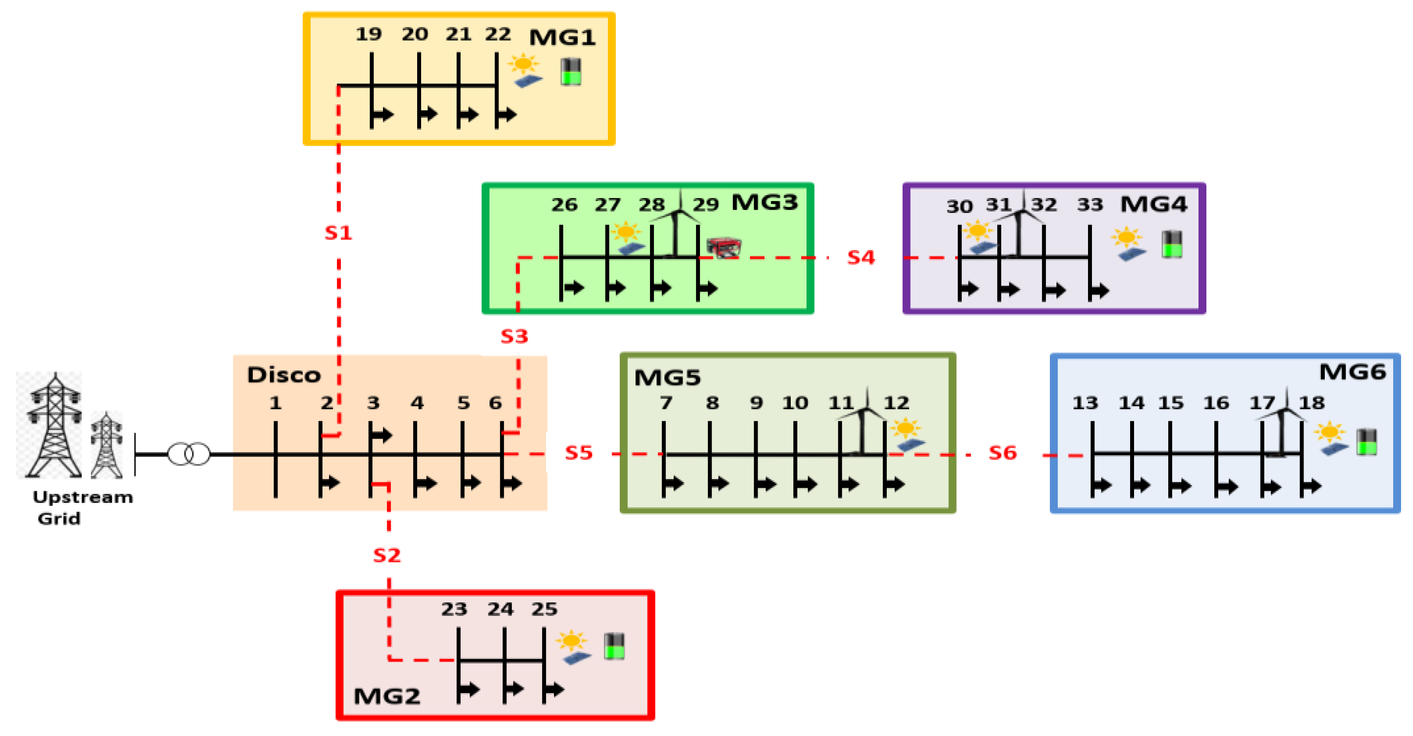
2. Proposed Work
3. Problem Formulation
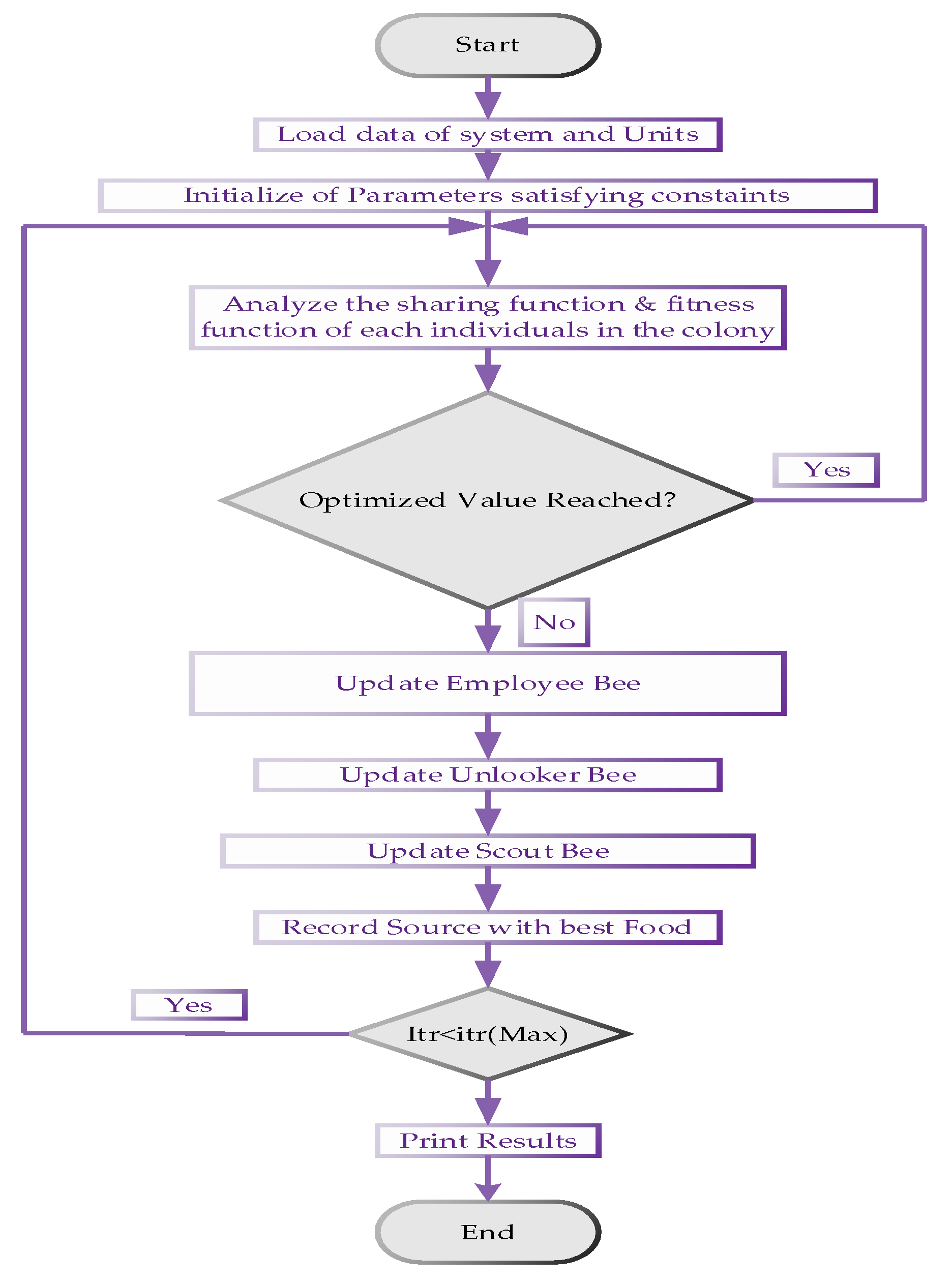
3.1. Artificial Bee Colony Algorithm
3.2. The ABC Algorithm Representation in Flowchart
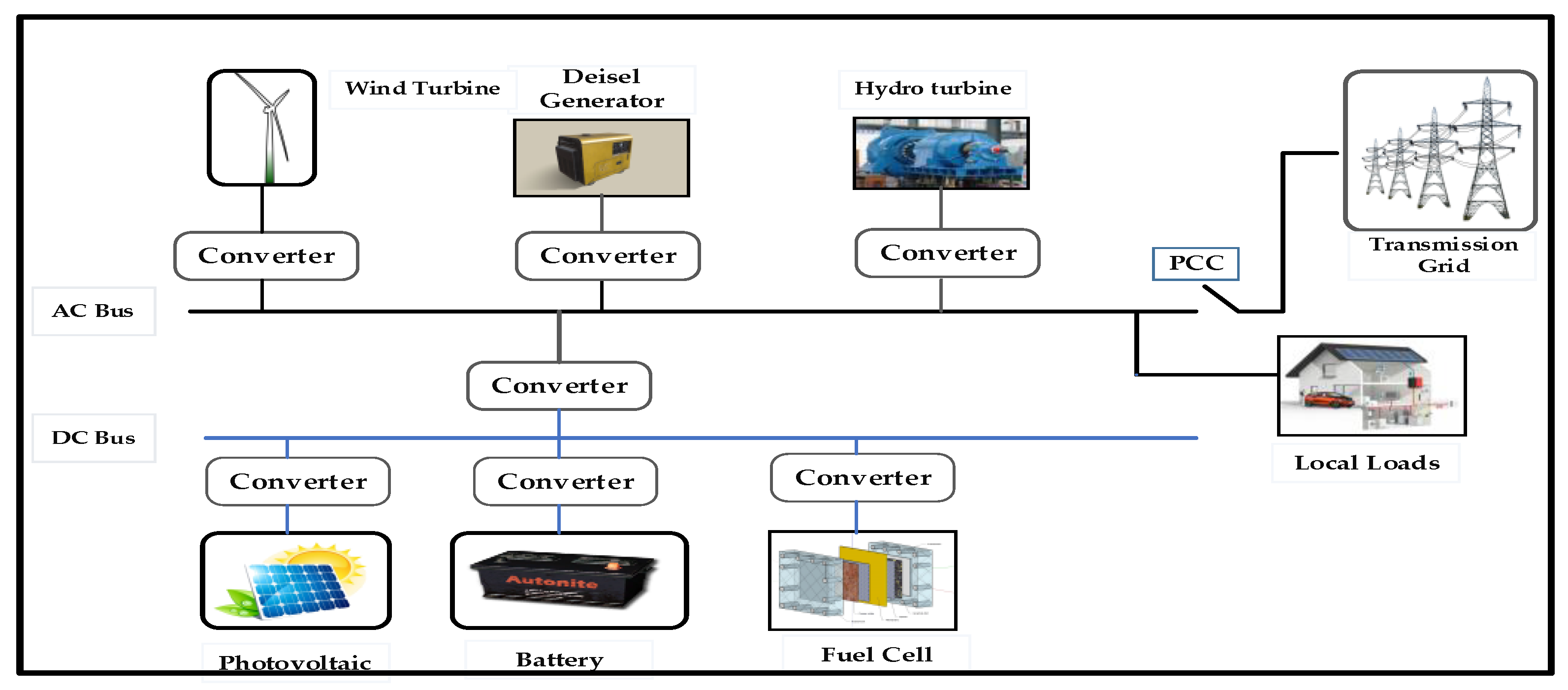
4. Mathematical Modeling of Microgrid Components
5. Methodology
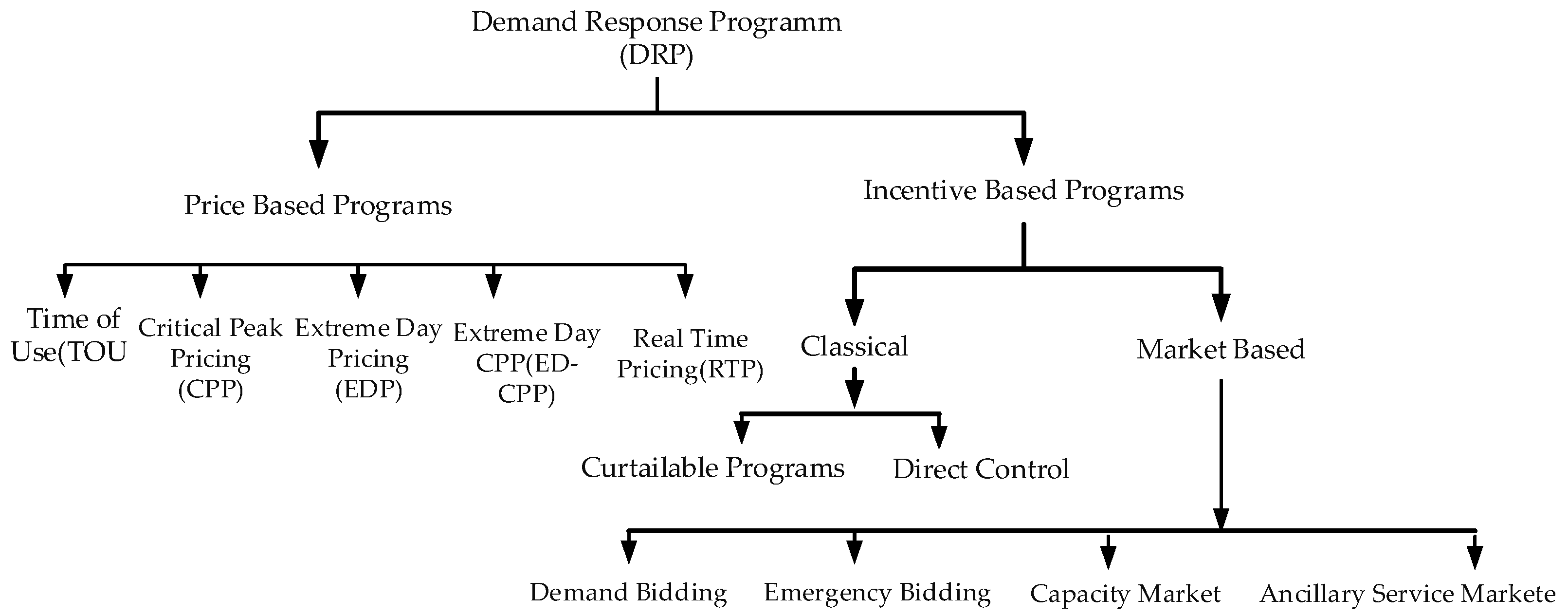
5.1. Demand Response
5.2. Elasticity
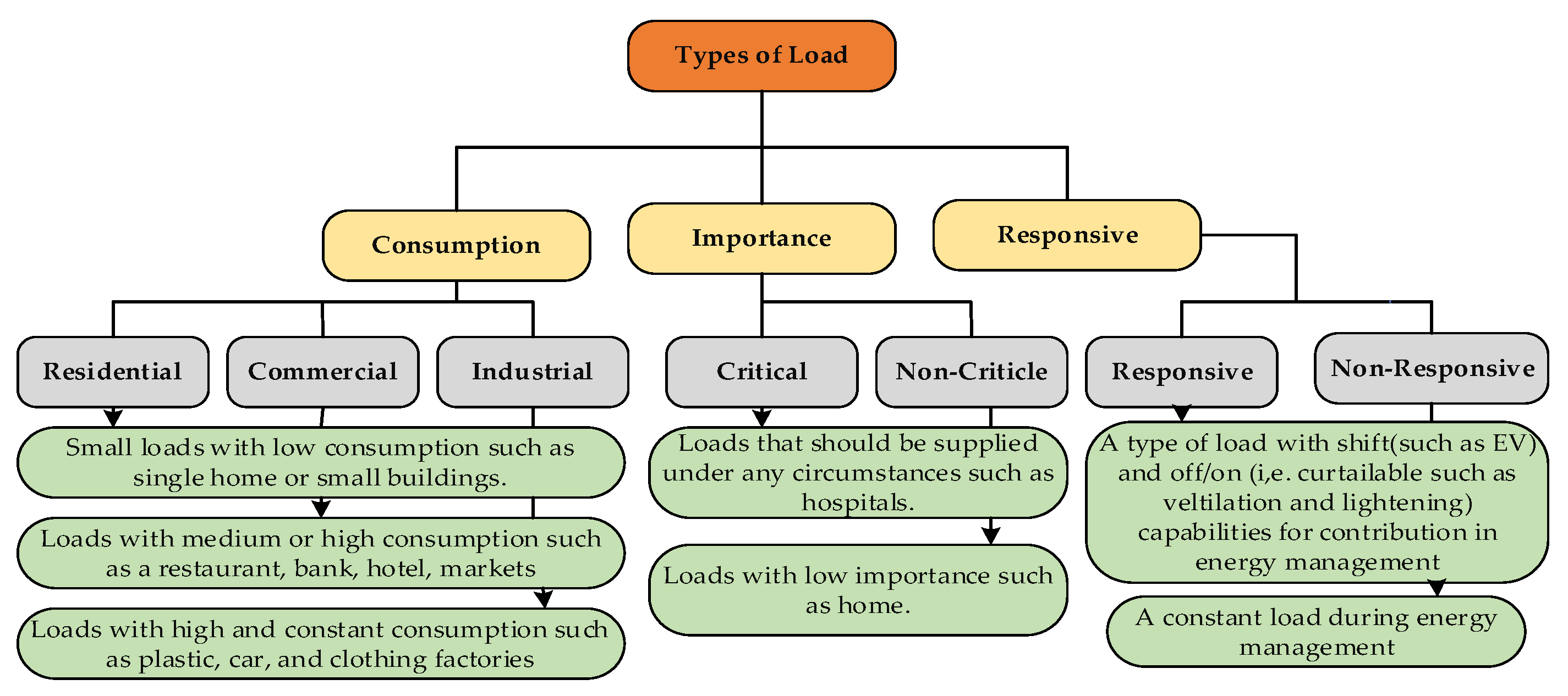
5.3. Types of Load
6. Proposed Model
6.1. Proposed Model Methodology
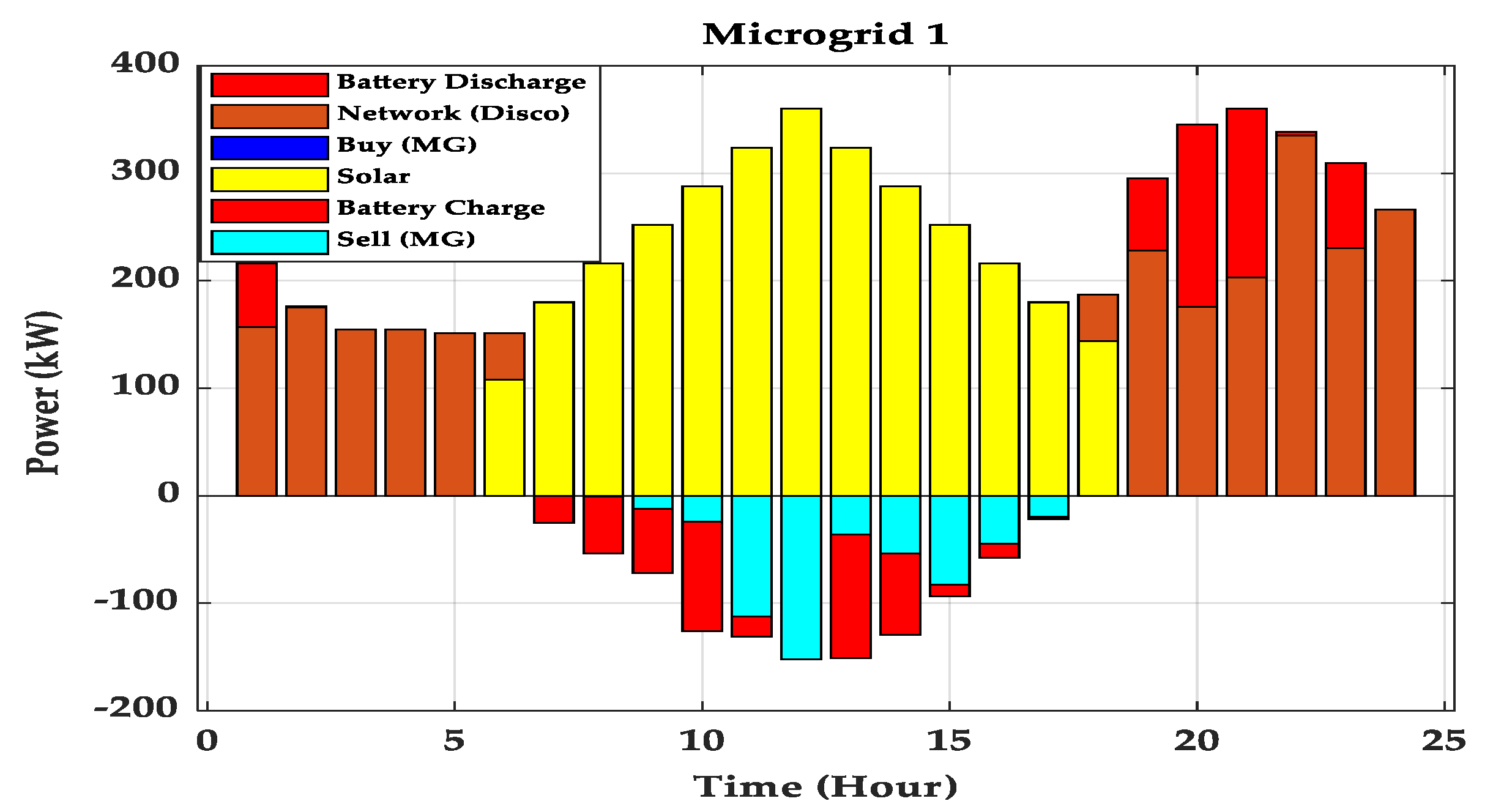
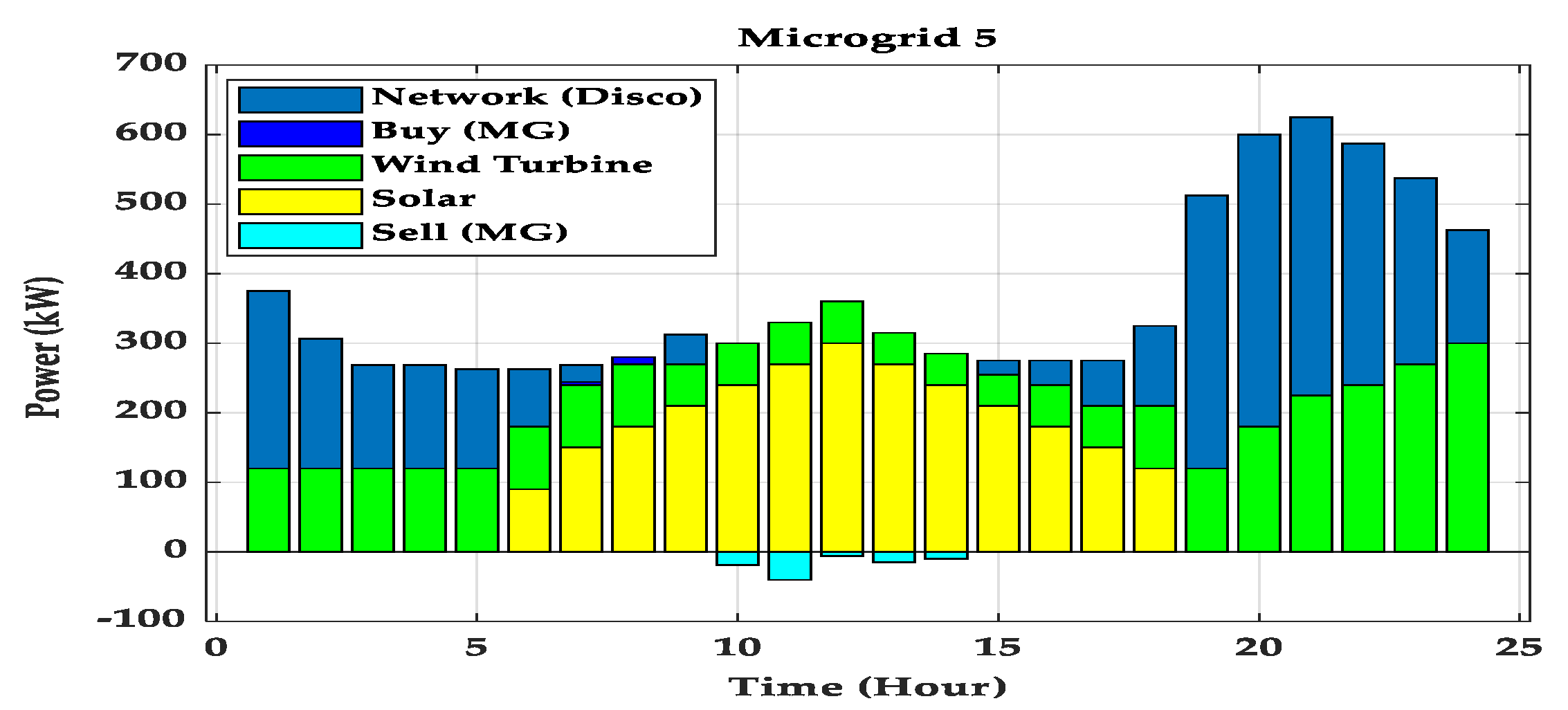
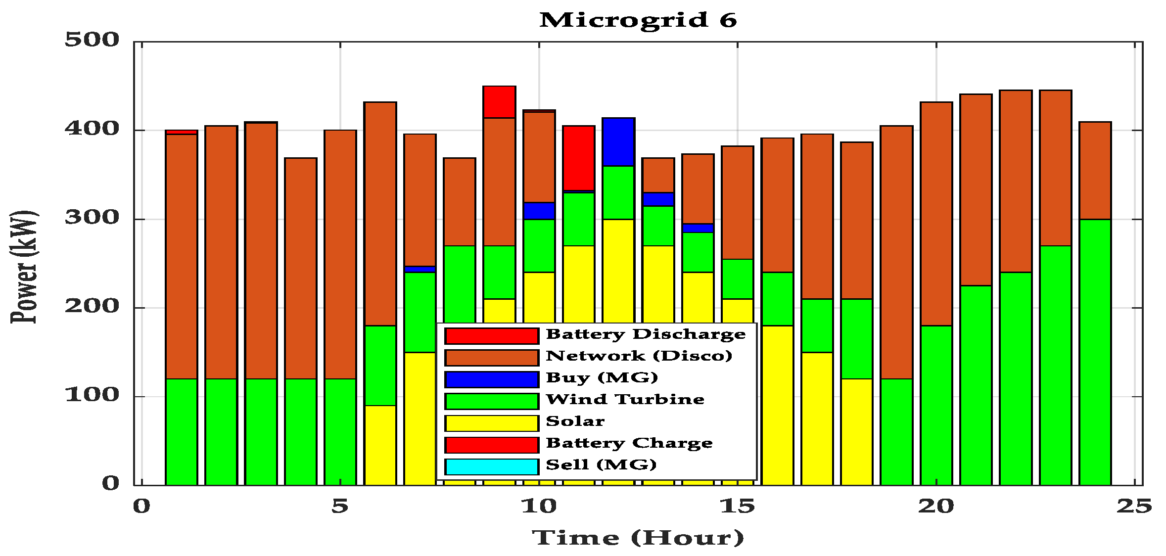
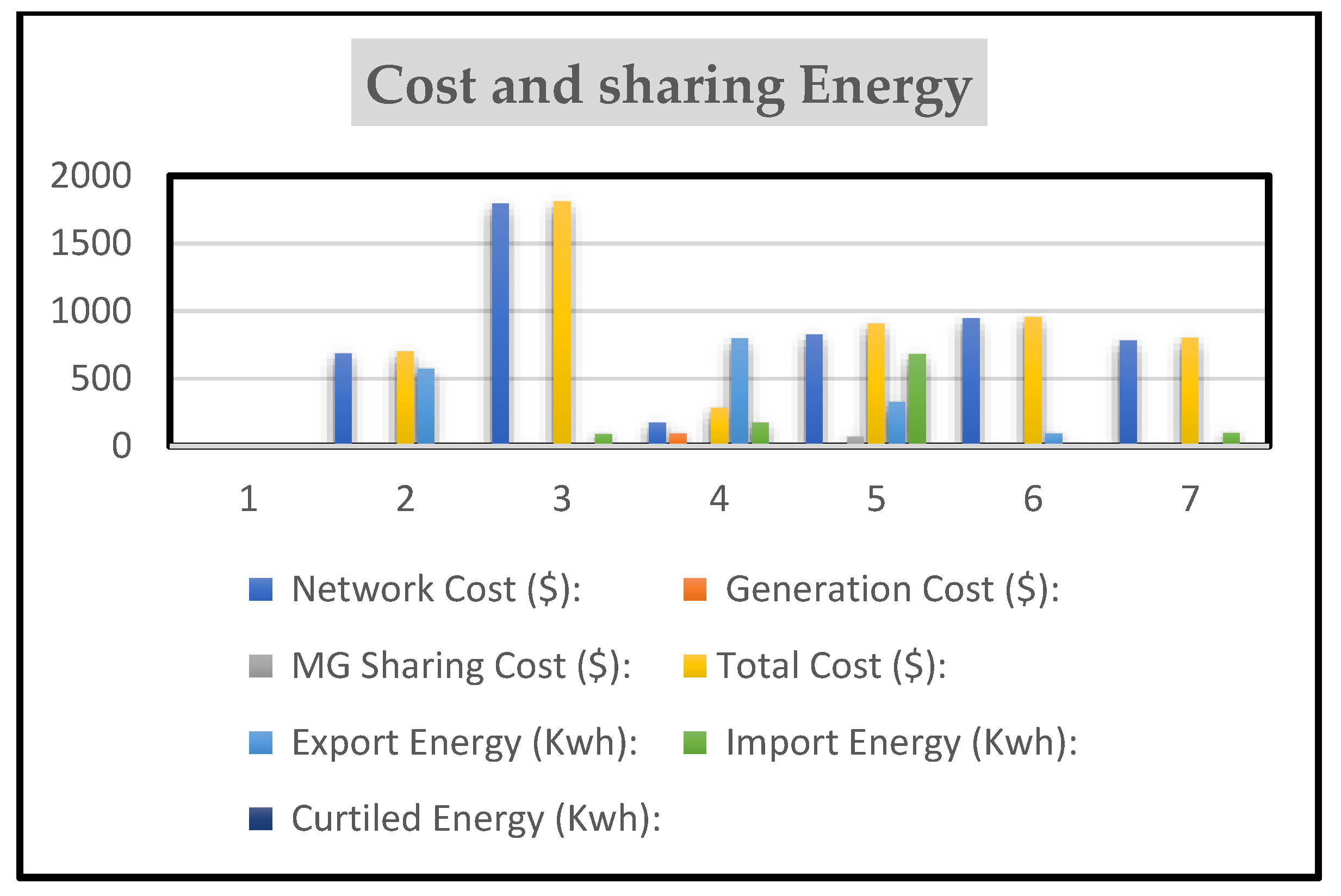
6.2. Power-Sharing, Costs, and Power Losses in Microgrids
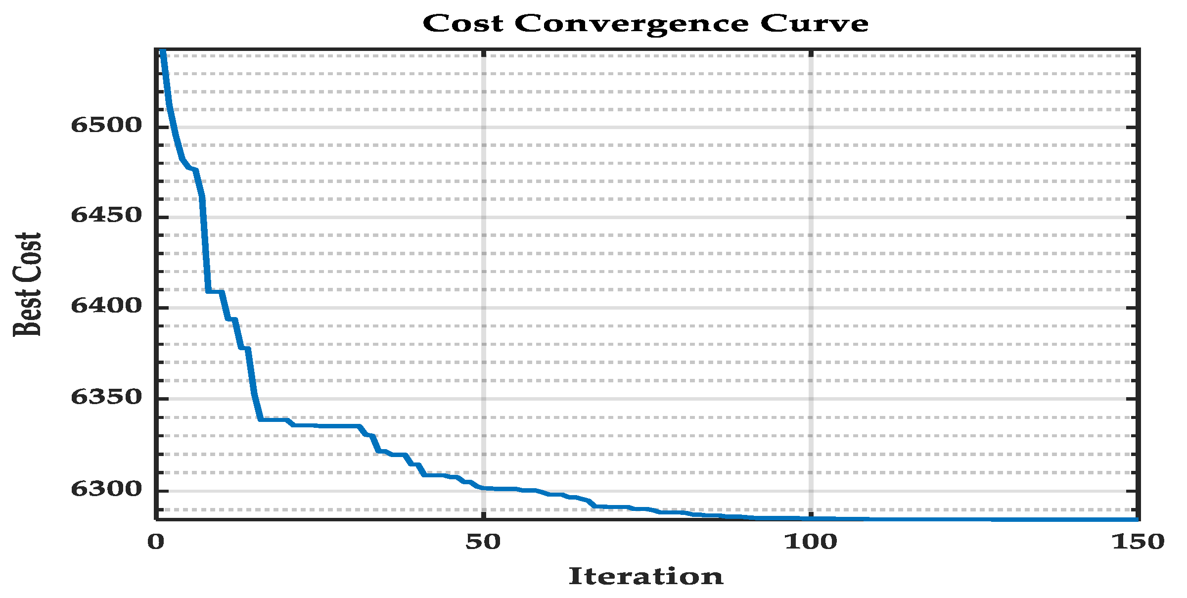
7. Results and Discussion
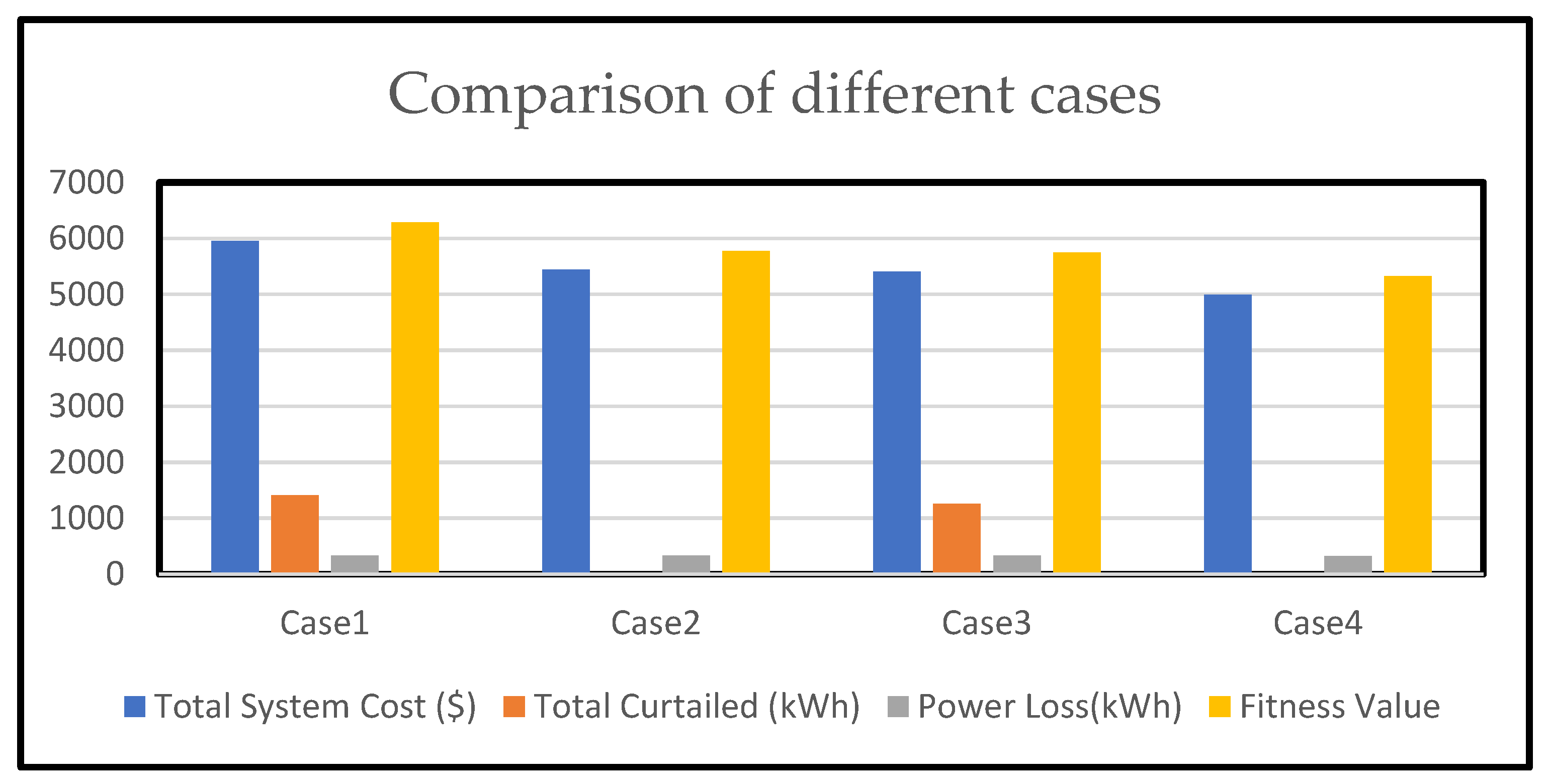
7.1. For Case 1, the Simulations for Cost
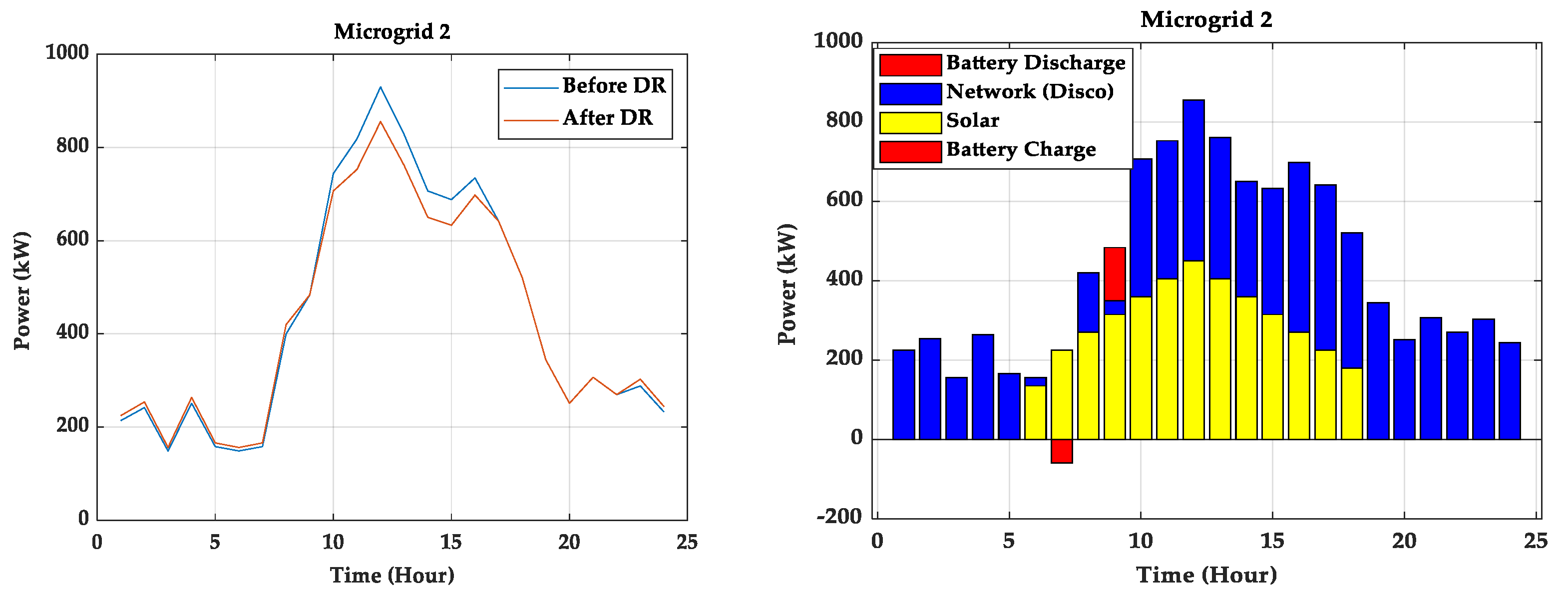
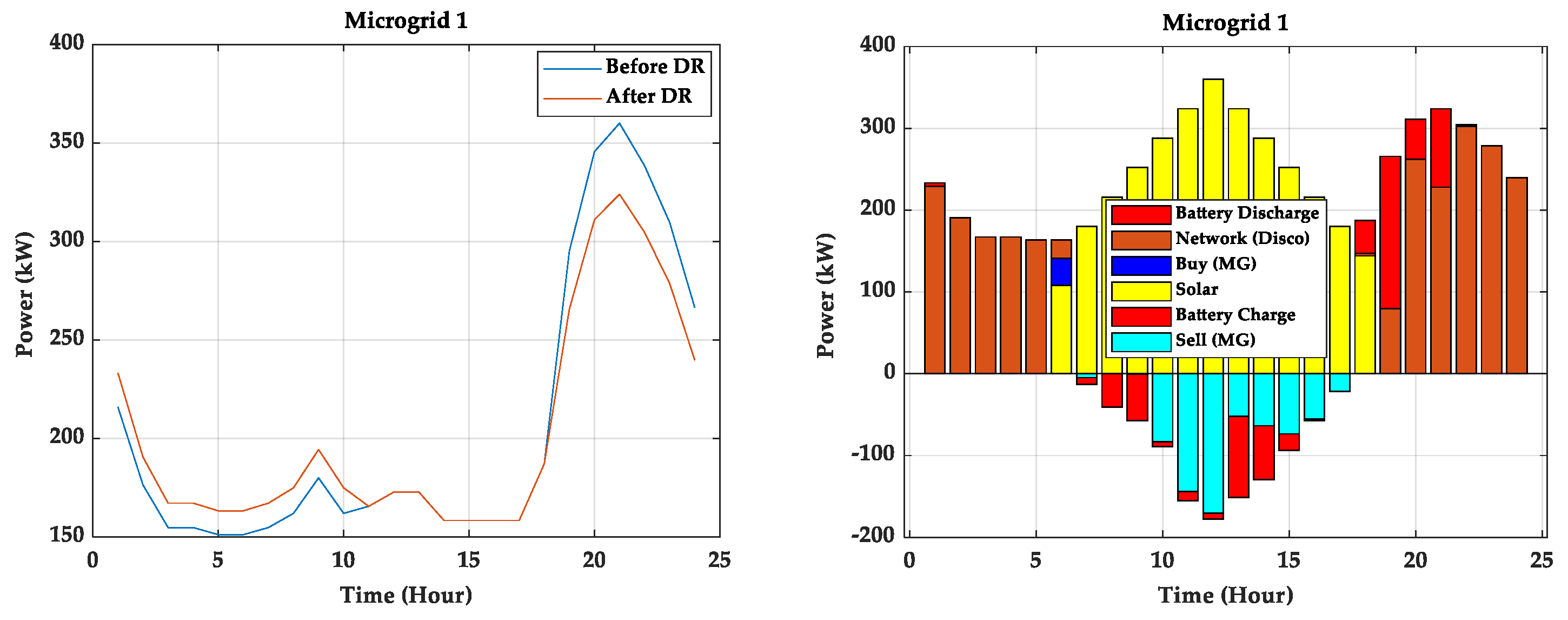
7.2. Case 2: Power-Sharing but Not Demand Response
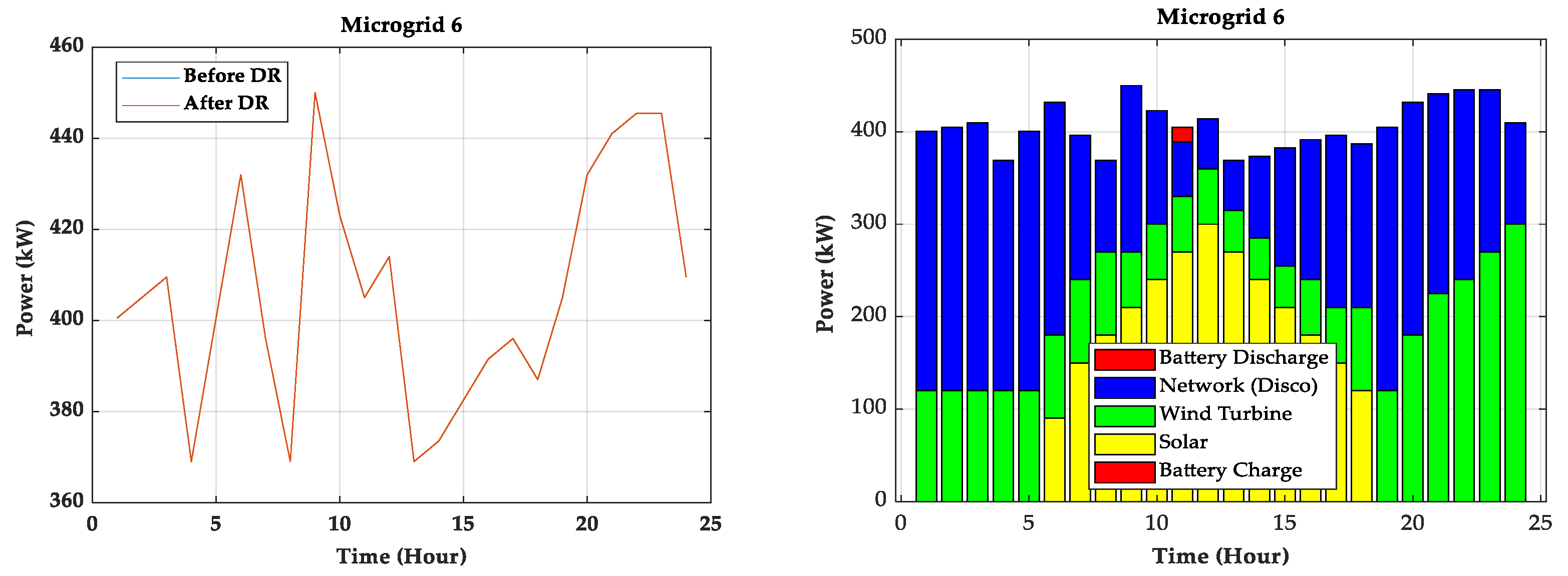
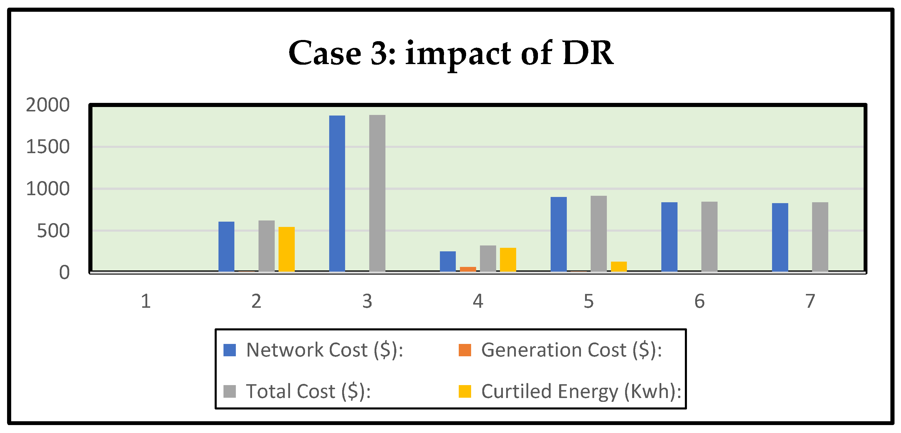
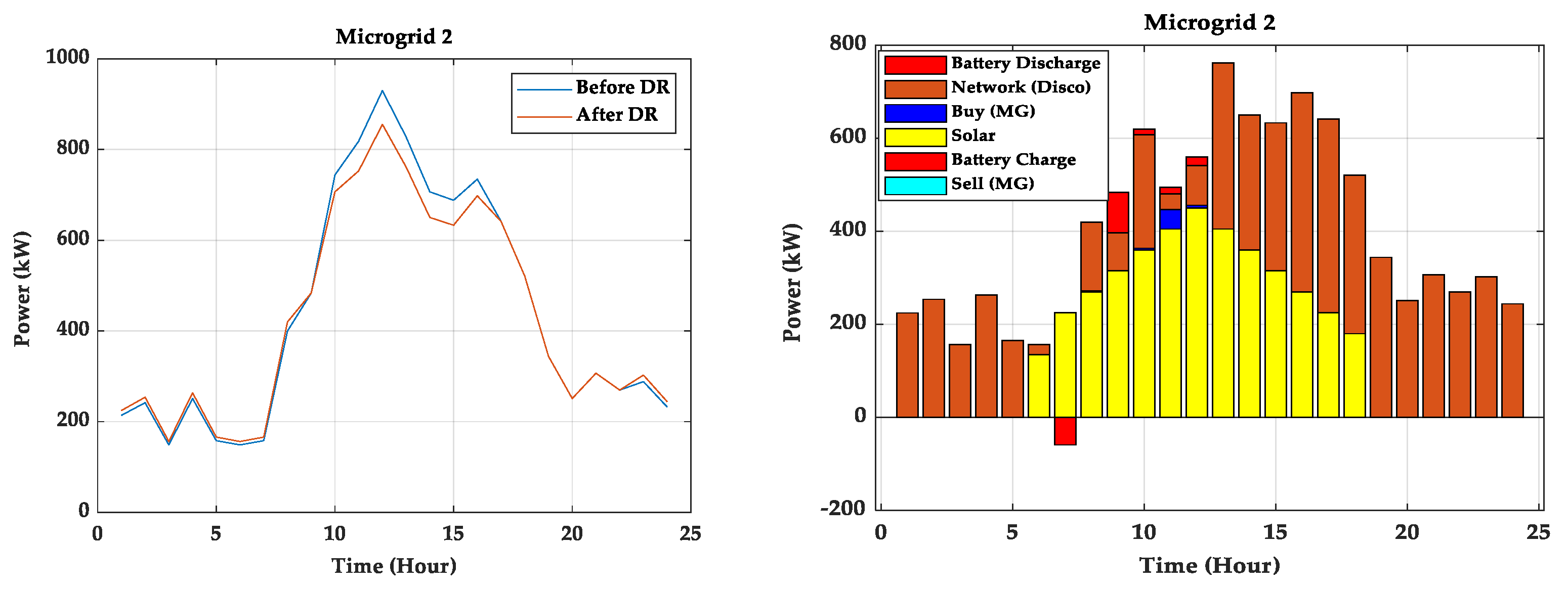
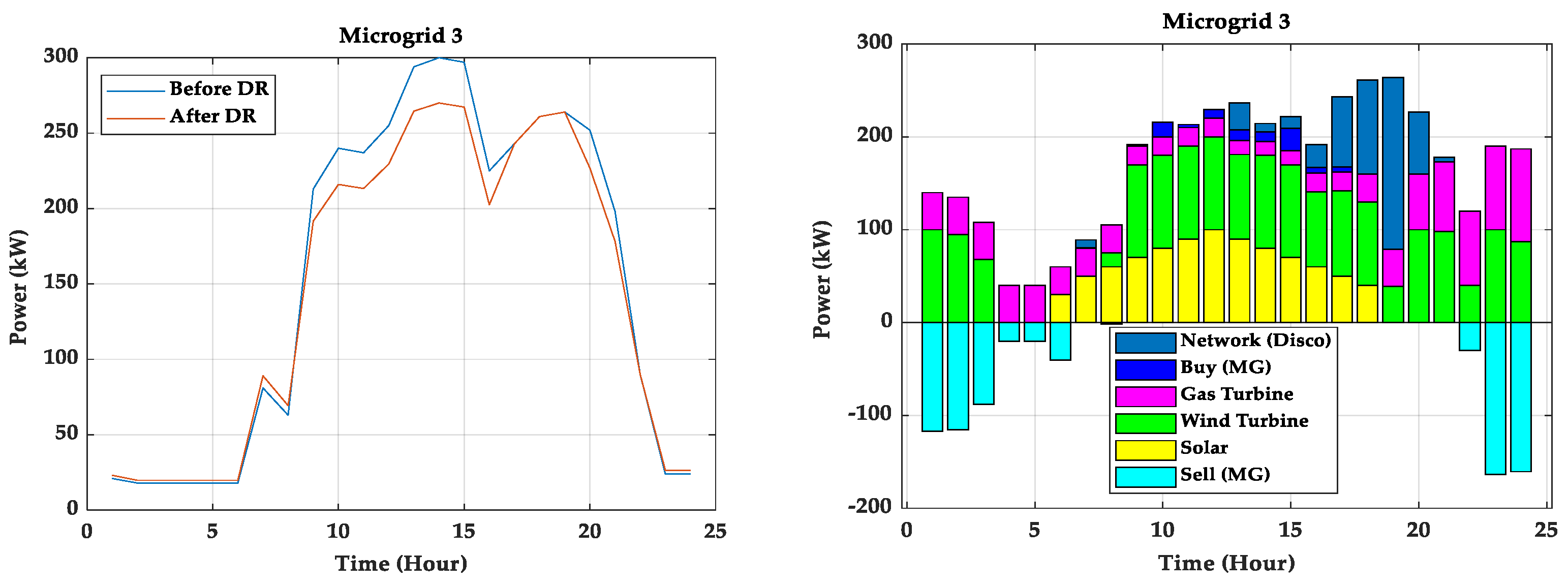
7.3. Case 3: Cost and Loss Calculations with DR but Not Power-Sharing
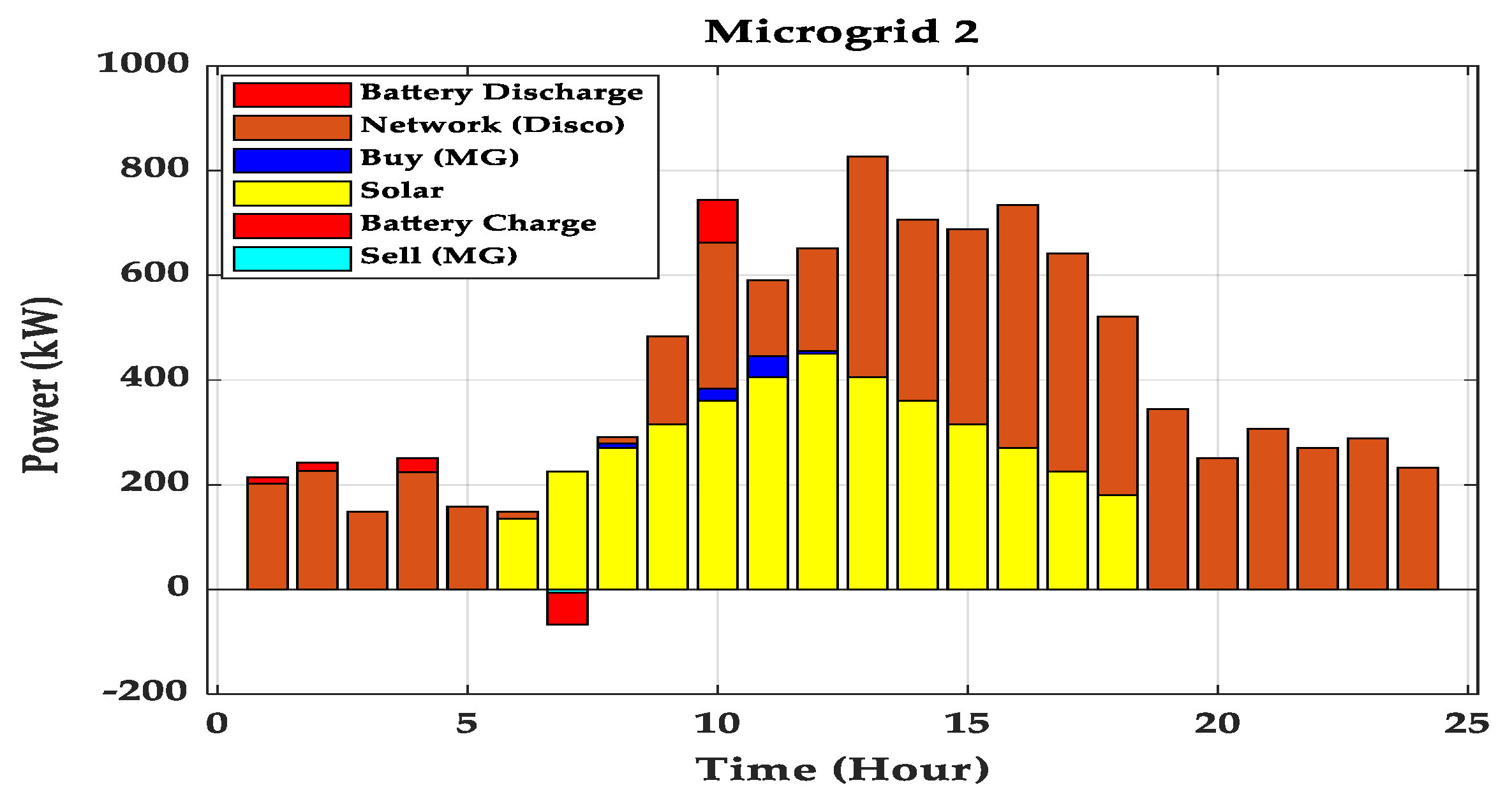
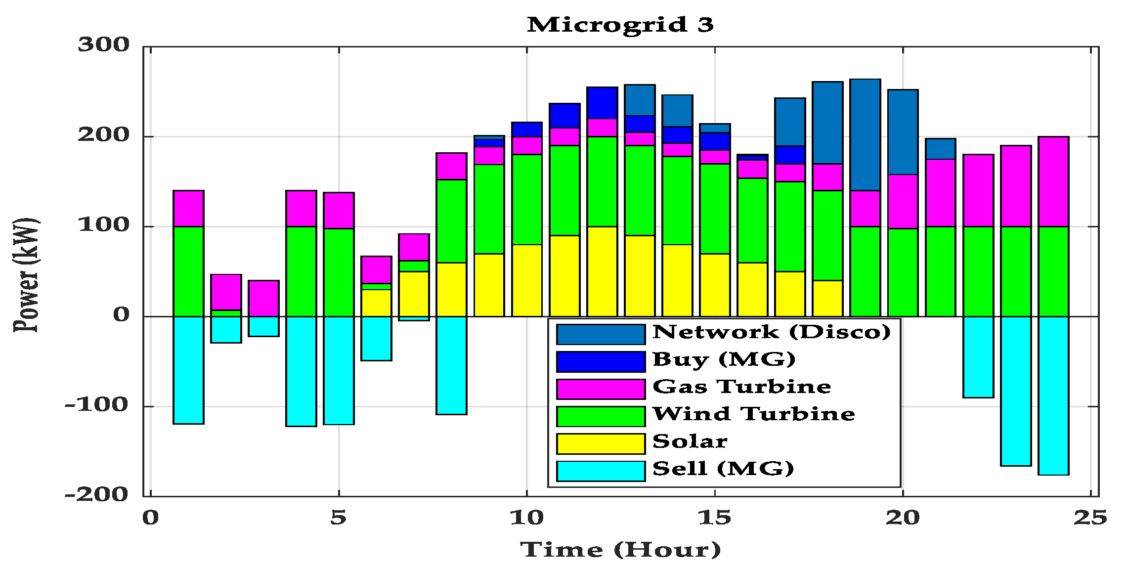
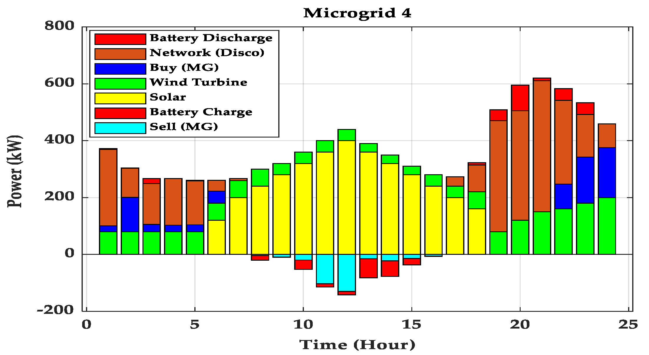
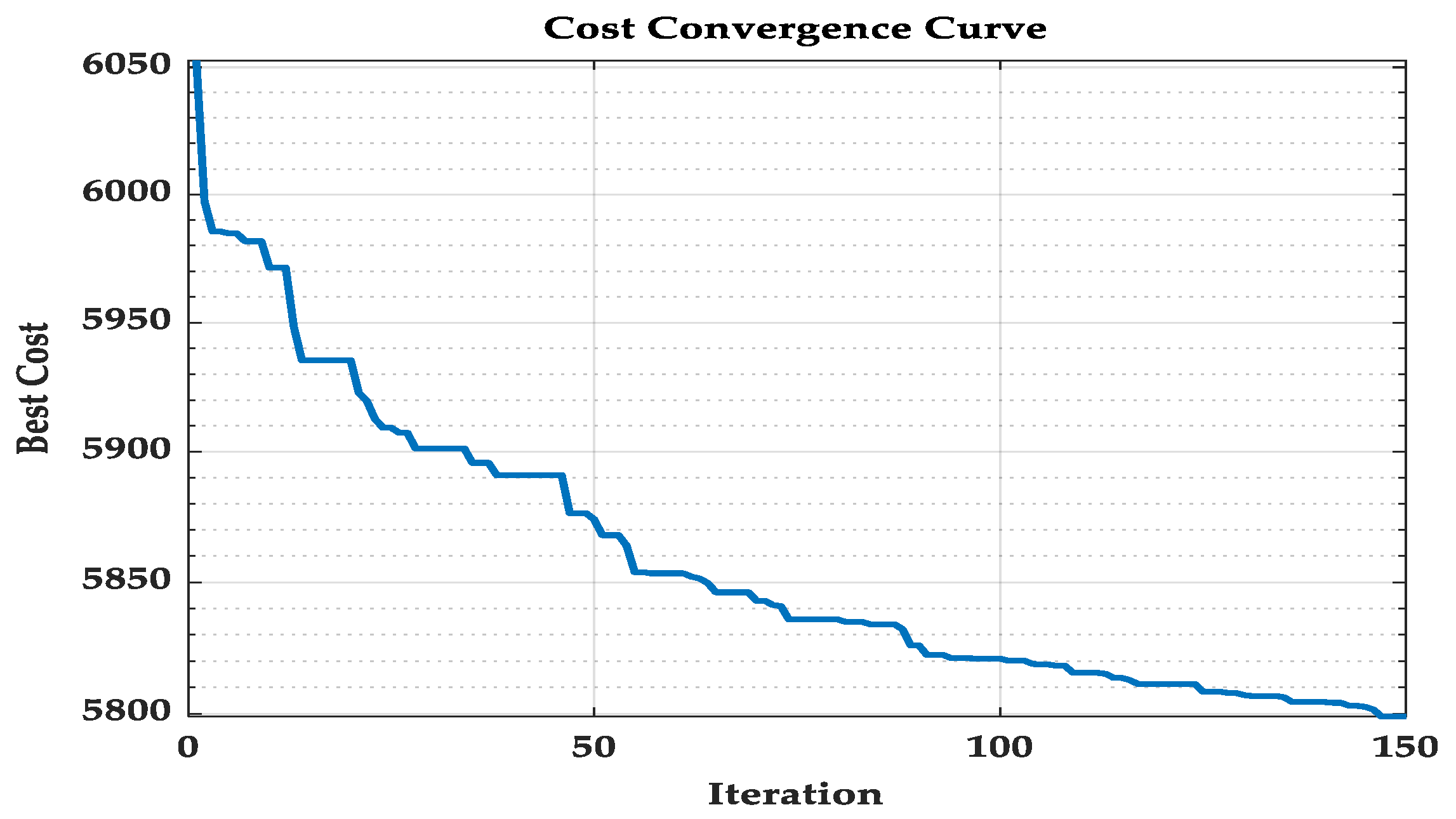
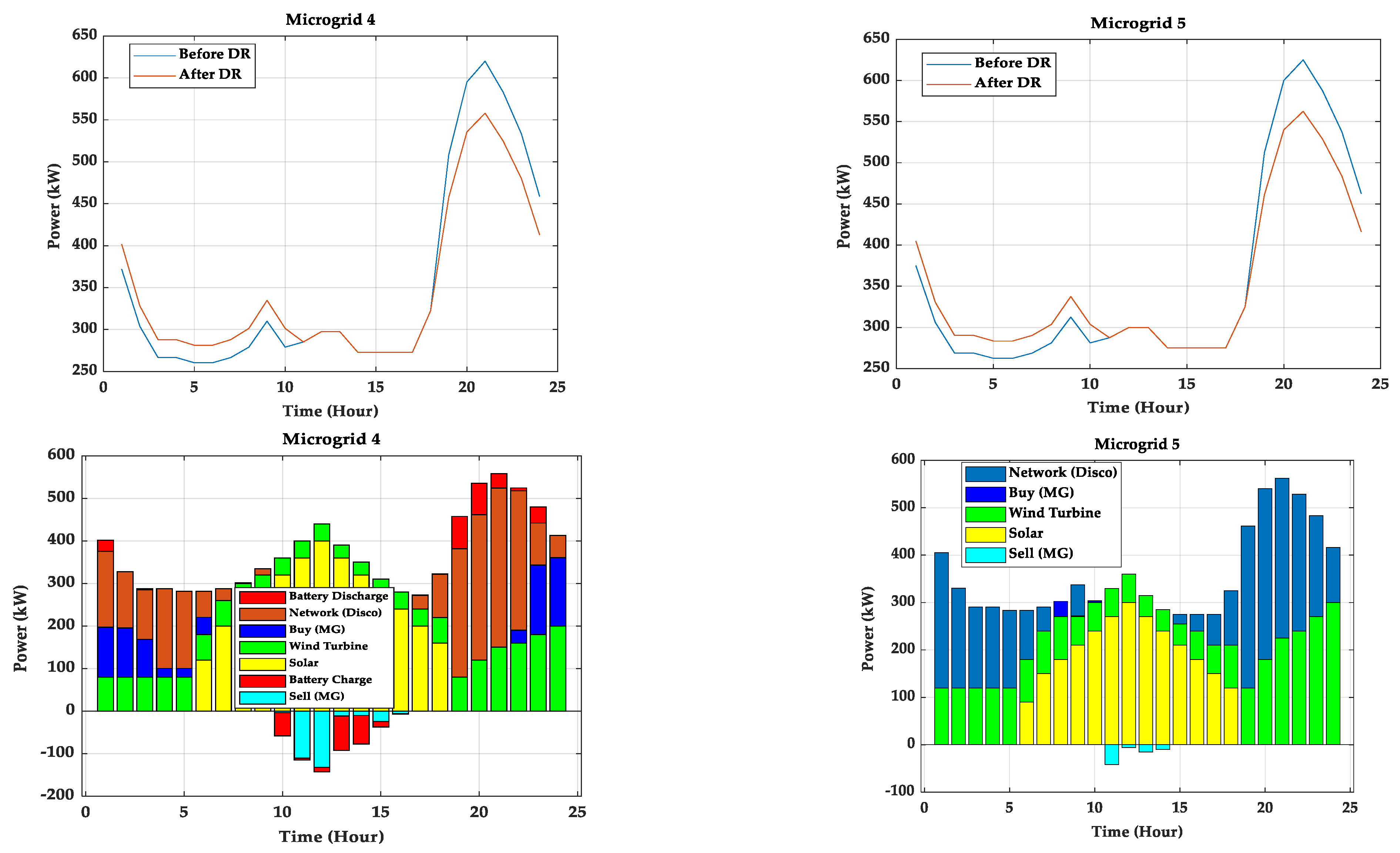
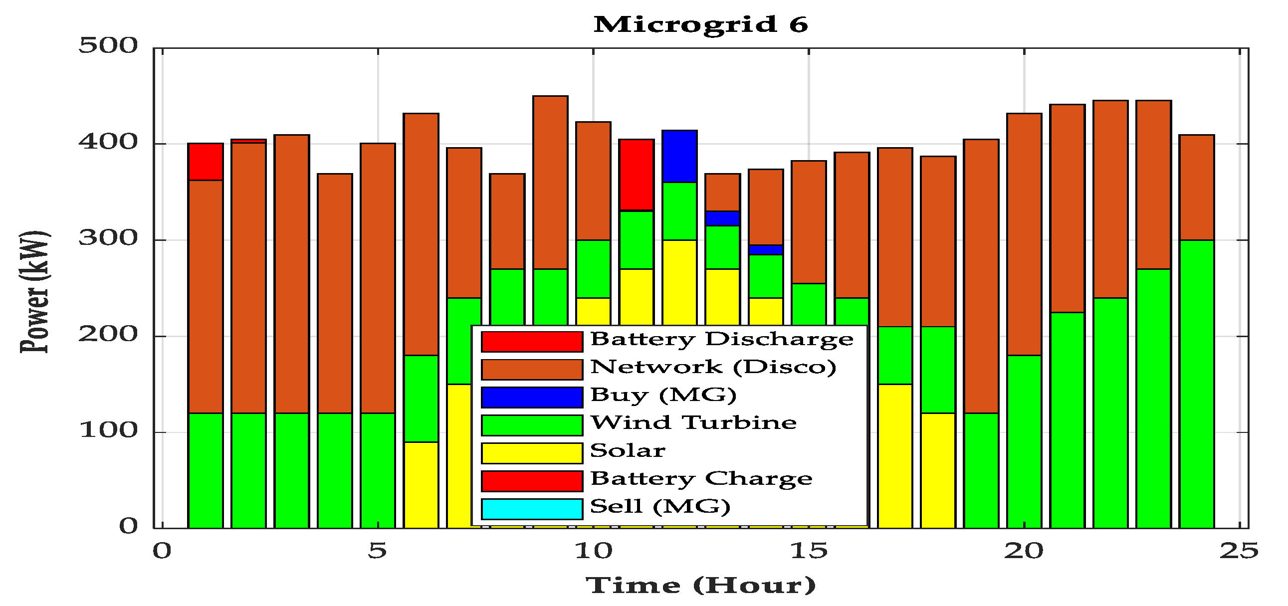
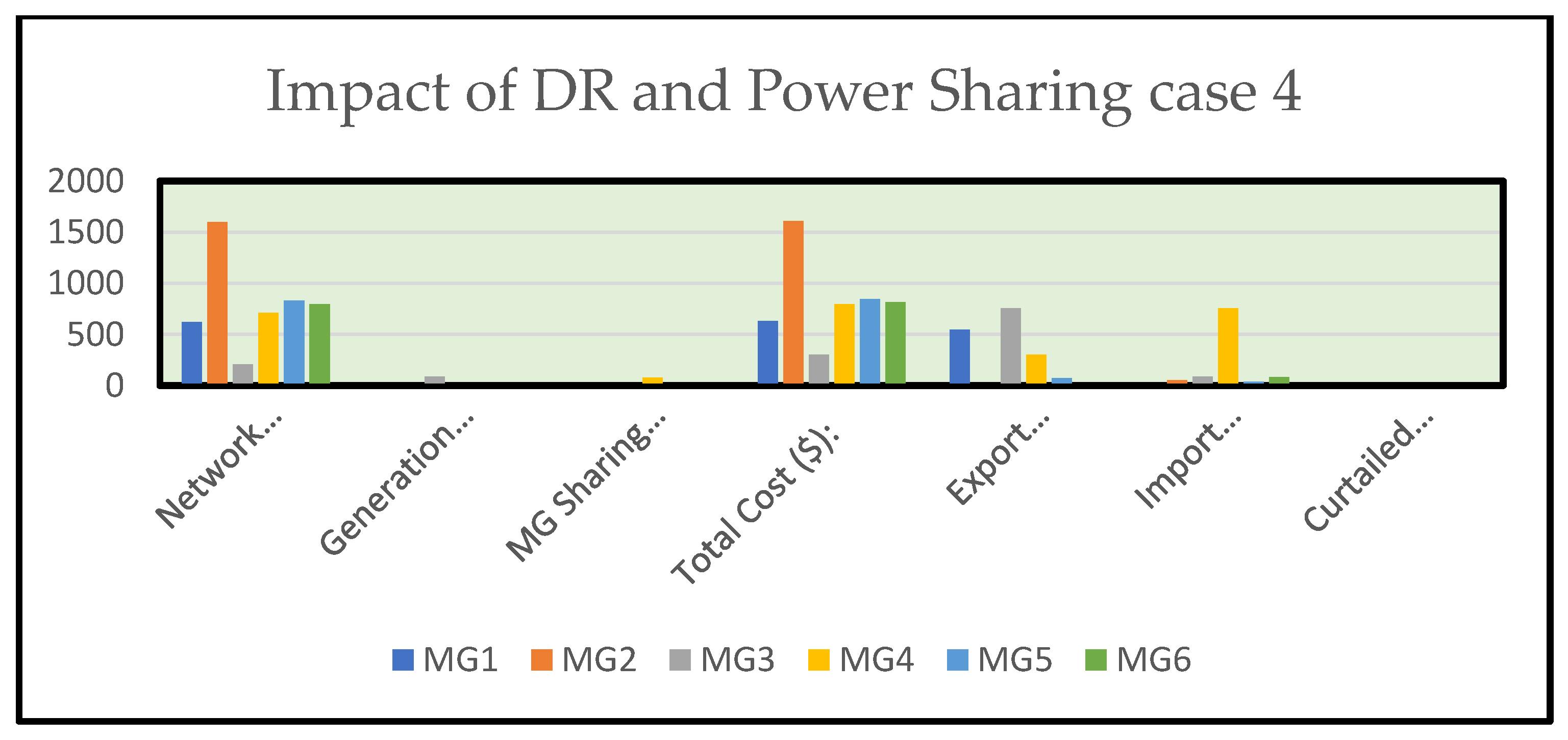
7.4. Case 4: Cost and Loss Calculations with DR and Power-Sharing
8. Conclusions
Author Contributions
Funding
Institutional Review Board Statement
Informed Consent Statement
Data Availability Statement
Conflicts of Interest
References
- Zhang, C.; Xu, Y.; Dong, Z.Y.; Wong, K.P. Robust Coordination of Distributed Generation and Price-Based Demand Response in Microgrids. IEEE Trans. Smart Grid 2018, 9, 4236–4247. [Google Scholar] [CrossRef]
- Robert, F.C.; Sisodia, G.S.; Gopalan, S. A critical review on the utilization of storage and demand response for the implementation of renewable energy microgrids. Sustain. Cities Soc. 2018, 40, 735–745. [Google Scholar] [CrossRef]
- Huang, S.; Abedinia, O. Investigation in economic analysis of microgrids based on renewable energy uncertainty and demand response in the electricity market. Energy 2021, 225, 120247. [Google Scholar] [CrossRef]
- Farsangi, A.S.; Hadayeghparast, S.; Mehdinejad, M.; Shayanfar, H. A novel stochastic energy management of a microgrid with various types of distributed energy resources in presence of demand response programs. Energy 2018, 160, 257–274. [Google Scholar] [CrossRef]
- Liu, N.; Yu, X.; Wang, C.; Li, C.; Ma, L.; Lei, J. Energy-Sharing Model with Price-Based Demand Response for Microgrids of Peer-to-Peer Prosumers. IEEE Trans. Power Syst. 2017, 32, 3569–3583. [Google Scholar] [CrossRef]
- Rajamand, S. Effect of demand response program of loads in cost optimization of microgrid considering uncertain parameters in PV/WT, market price and load demand. Energy 2020, 194, 116917. [Google Scholar] [CrossRef]
- Hassan, M.A.S.; Chen, M.; Lin, H.; Ahmed, M.H.; Khan, M.Z.; Chughtai, G.R. Optimization modeling for dynamic price based demand response in microgrids. J. Clean. Prod. 2019, 222, 231–241. [Google Scholar] [CrossRef]
- Sabzehgar, R.; Kazemi, M.A.; Rasouli, M.; Fajri, P. Cost optimization and reliability assessment of a microgrid with large-scale plug-in electric vehicles participating in demand response programs. Int. J. Green Energy 2020, 17, 127–136. [Google Scholar] [CrossRef]
- Li, C.; Jia, X.; Zhou, Y.; Li, X. A microgrids energy management model based on multi-agent system using adaptive weight and chaotic search particle swarm optimization considering demand response. J. Clean. Prod. 2020, 262, 121247. [Google Scholar] [CrossRef]
- Wang, Y.; Huang, Y.; Wang, Y.; Li, F.; Zhang, Y.; Tian, C. Operation Optimization in a Smart Micro-Grid in the Presence of Distributed Generation and Demand Response. Sustainability 2018, 10, 847. [Google Scholar] [CrossRef] [Green Version]
- Faia, R.; Canizes, B.; Faria, P.; Vale, Z.; Terras, J.M.; Cunha, L.V. Optimal Distribution Grid Operation Using Demand Response. In Proceedings of the IEEE PES Innovative Smart Grid Technologies Conference NA (ISGT NA), Washington, DC, USA, 17–20 February 2020. [Google Scholar] [CrossRef]
- Helmi, A.M.; Carli, R.; Dotoli, M.; Ramadan, H.S. Efficient and Sustainable Reconfiguration of Distribution Networks via Metaheuristic Optimization. IEEE Trans. Autom. Sci. Eng. 2021, 19, 82–98. [Google Scholar] [CrossRef]
- Muhammad, M.A.; Mokhlis, H.; Naidu, K.; Amin, A.; Franco, J.F.; Othman, M. Distribution Network Planning Enhancement via Network Reconfiguration and DG Integration Using Dataset Approach and Water Cycle Algorithm. J. Mod. Power Syst. Clean Energy 2020, 8, 86–93. [Google Scholar] [CrossRef]
- Zhao, H.; Lu, H.; Li, B.; Wang, X.; Zhang, S.; Wang, Y. Stochastic Optimization of Microgrid Participating Day-Ahead Market Operation Strategy with Consideration of Energy Storage System and Demand Response. Energies 2020, 13, 1255. [Google Scholar] [CrossRef] [Green Version]
- Murty, V.V.S.N.; Kumar, A. Multi-objective energy management in microgrids with hybrid energy sources and battery energy storage systems. Prot. Control Mod. Power Syst. 2020, 5, 1–20. [Google Scholar] [CrossRef] [Green Version]
- Nasr, M.-A.; Nikkhah, S.; Gharehpetian, G.B.; Nasr-Azadani, E.; Hosseinian, S.H. A multi-objective voltage stability constrained energy management system for isolated microgrids. Int. J. Electr. Power Energy Syst. 2020, 117, 105646. [Google Scholar] [CrossRef]
- Mansouri, S.A.; Ahmarinejad, A.; Nematbakhsh, E.; Javadi, M.S.; Jordehi, A.R.; Catalão, J.P. Energy management in microgrids including smart homes: A multi-objective approach. Sustain. Cities Soc. 2021, 69, 102852. [Google Scholar] [CrossRef]
- Nguyen, A.-D.; Bui, V.-H.; Hussain, A.; Nguyen, D.-H.; Kim, H.-M. Impact of Demand Response Programs on Optimal Operation of Multi-Microgrid System. Energies 2018, 11, 1452. [Google Scholar] [CrossRef] [Green Version]
- Shafiee, M.; Rashidinejad, M.; Abdollahi, A.; Ghaedi, A. A novel stochastic framework based on PEM-DPSO for optimal operation of microgrids with demand response. Sustain. Cities Soc. 2021, 72, 103024. [Google Scholar] [CrossRef]
- Albadi, M.H.; El-Saadany, E.F. Demand response in electricity markets: An overview. In Proceedings of the 2007 IEEE Power Engineering Society General Meeting, PES, Bellevue, WA, USA, 24 June 2007. [Google Scholar]
- Carli, R.; Cavone, G.; Pippia, T.; De Schutter, B.; Dotoli, M. Robust Optimal Control for Demand Side Management of Multi-Carrier Microgrids. TechRxiv 2022. Preprint. [Google Scholar] [CrossRef]
- Barbato, A.; Capone, A. Optimization Models and Methods for Demand-Side Management of Residential Users: A Survey. Energies 2014, 7, 5787–5824. [Google Scholar] [CrossRef]
- Astriani, Y.; Shafiullah, G.; Shahnia, F. Incentive determination of a demand response program for microgrids. Appl. Energy 2021, 292, 116624. [Google Scholar] [CrossRef]
- Javanmard, B.; Tabrizian, M.; Ansarian, M.; Ahmarinejad, A. Energy management of multi-microgrids based on game theory approach in the presence of demand response programs, energy storage systems and renewable energy resources. J. Energy Storage 2021, 42, 102971. [Google Scholar] [CrossRef]
- Imani, M.H.; Ghadi, M.J.; Ghavidel, S.; Li, L. Demand Response Modeling in Microgrid Operation: A Review and Application for Incentive-Based and Time-Based Programs. Renew. Sustain. Energy Rev. 2018, 94, 486–499. [Google Scholar] [CrossRef]
- Guo, Q.; Liang, X.; Xie, D.; Jermsittiparsert, K. Efficient integration of demand response and plug-in electrical vehicle in microgrid: Environmental and economic assessment. J. Clean. Prod. 2021, 291, 125581. [Google Scholar] [CrossRef]
- Mohseni, S.; Brent, A.C.; Burmester, D. A demand response-centred approach to the long-term equipment capacity planning of grid-independent micro-grids optimized by the moth-flame optimization algorithm. Energy Convers. Manag. 2019, 200, 112105. [Google Scholar] [CrossRef]
- Harsh, P.; Das, D. Energy management in microgrid using incentive-based demand response and reconfigured network considering uncertainties in renewable energy sources. Sustain. Energy Technol. Assess. 2021, 46, 101225. [Google Scholar] [CrossRef]
- Dou, C.; Zhou, X.; Zhang, T.; Xu, S. Economic Optimization Dispatching Strategy of Microgrid for Promoting Photoelectric Consumption Considering Cogeneration and Demand Response. J. Mod. Power Syst. Clean Energy 2020, 8, 557–563. [Google Scholar] [CrossRef]
- Ghose, T.; Pandey, H.W.; Gadham, K.R. Risk assessment of microgrid aggregators considering demand response and uncertain renewable energy sources. J. Mod. Power Syst. Clean Energy 2019, 7, 1619–1631. [Google Scholar] [CrossRef] [Green Version]
- Faraji, J.; Ketabi, A.; Hashemi-Dezaki, H.; Shafie-Khah, M.; Catalao, J.P.S. Optimal Day-Ahead Self-Scheduling and Operation of Prosumer Microgrids Using Hybrid Machine Learning-Based Weather and Load Forecasting. IEEE Access 2020, 8, 157284–157305. [Google Scholar] [CrossRef]
- Hemmati, M.; Mirzaei, M.A.; Abapour, M.; Zare, K.; Mohammadi-Ivatloo, B.; Mehrjerdi, H.; Marzband, M. Economic-environmental analysis of combined heat and power-based reconfigurable microgrid integrated with multiple energy storage and demand response program. Sustain. Cities Soc. 2021, 69, 102790. [Google Scholar] [CrossRef]
- Fouladfar, M.H.; Loni, A.; Tookanlou, M.B.; Marzband, M.; Godina, R.; Al-Sumaiti, A.; Pouresmaeil, E. The Impact of Demand Response Programs on Reducing the Emissions and Cost of a Neighborhood Home Microgrid. Appl. Sci. 2019, 9, 2097. [Google Scholar] [CrossRef] [Green Version]
- Ahmadi, S.E.; Rezaei, N. A new isolated renewable based multi microgrid optimal energy management system considering uncertainty and demand response. Int. J. Electr. Power Energy Syst. 2020, 118, 105760. [Google Scholar] [CrossRef]
- Karimi, H.; Jadid, S.; Karimi, H.; Jadid, S. Optimal energy management for multi-microgrid considering demand response programs: A stochastic multi-objective framework. Energy 2020, 195, 116992. [Google Scholar] [CrossRef]
- Nayak, A.; Maulik, A.; Das, D. An integrated optimal operating strategy for a grid-connected AC microgrid under load and renewable generation uncertainty considering demand response. Sustain. Energy Technol. Assess. 2021, 45, 101169. [Google Scholar] [CrossRef]
- da Silva, I.R.S.; Rabêlo, R.D.A.; Rodrigues, J.J.; Solic, P.; Carvalho, A. A preference-based demand response mechanism for energy management in a microgrid. J. Clean. Prod. 2020, 255, 120034. [Google Scholar] [CrossRef]
- Ajoulabadi, A.; Ravadanegh, S.N.; Mohammadi-Ivatloo, B. Flexible scheduling of reconfigurable microgrid-based distribution networks considering demand response program. Energy 2020, 196, 117024. [Google Scholar] [CrossRef]
- Chen, S.-M.; Sarosh, A.; Dong, Y.-F. Simulated annealing based artificial bee colony algorithm for global numerical optimization. Appl. Math. Comput. 2012, 219, 3575–3589. [Google Scholar] [CrossRef]
- Zhang, C.; Zheng, J.; Zhou, Y. Two modified Artificial Bee Colony algorithms inspired by Grenade Explosion Method. Neurocomputing 2015, 151, 1198–1207. [Google Scholar] [CrossRef]
- Yang, X.S. Engineering Optimization: An Introduction with Metaheuristic Applications; John Wily & Sons: Hoboken, NJ, USA, 2010. [Google Scholar]
- Aissou, S.; Rekioua, D.; Mezzai, N.; Rekioua, T.; Bacha, S. Modeling and control of hybrid photovoltaic wind power system with battery storage. Energy Convers. Manag. 2015, 89, 615–625. [Google Scholar] [CrossRef]
- Moradi, M.H.; Eskandari, M. A hybrid method for simultaneous optimization of DG capacity and operational strategy in microgrids considering uncertainty in electricity price forecasting. Renew. Energy 2014, 68, 697–714. [Google Scholar] [CrossRef]
- Polit, U.; Facultat, C.; Gonz, I. Optimal Management of Microgrids. Master’s Thesis, Universitat Politècnica de Catalunya, Barcelona, Spain, 2012. [Google Scholar]
- Ullah, K.; Jiang, Q.; Geng, G.; Rahim, S.; Khan, R.A. Optimal Power Sharing in Microgrids Using the Artificial Bee Colony Algorithm. Energies 2022, 15, 1067. [Google Scholar] [CrossRef]
- Aalami, H.A.; Moghaddam, M.P.; Yousefi, G. Modeling and prioritizing demand response programs in power markets. Electr. Power Syst. Res. 2010, 80, 426–435. [Google Scholar] [CrossRef]
- Aalami, H.A.; Moghaddam, M.P.; Yousefi, G. Demand response modeling considering Interruptible/Curtailable loads and capacity market programs. Appl. Energy 2010, 87, 243–250. [Google Scholar] [CrossRef]


| References | Objective Function | Wind Turbine | PV | EES | Demand Response | Electric Vehicles |
|---|---|---|---|---|---|---|
| [24] | Power loss, VDI | ✓ | ✓ | ✓ | ✓ | |
| [25] | DRP’s to control system operation | ✓ | ✓ | ✓ | ✓ | |
| [26] | DRP(TOU) and EV’s for economic and environmental assessment. | ✓ | ✓ | ✓ | ||
| [27] | Optimal sizing of microgrid. | ✓ | ✓ | ✓ | ✓ | ✓ |
| [28] | Cost | ✓ | ✓ | ✓ | ||
| [29] | Cost | ✓ | ✓ | ✓ | ||
| [30] | Cost | ✓ | ✓ | ✓ | ||
| [31] | Cost | ✓ | ✓ | ✓ | ✓ | |
| [32] | Cost and emissions | ✓ | ✓ | ✓ | ✓ | |
| [33] | Cost and emissions | ✓ | ✓ | ✓ | ✓ | ✓ |
| [34] | Cost | ✓ | ✓ | ✓ | ✓ | |
| [35] | Losses and emissions | ✓ | ✓ | ✓ | ✓ | |
| [36] | Stability, cost, emissions | ✓ | ✓ | ✓ | ✓ | |
| [37] | Cost, stability, pollution | ✓ | ✓ | ✓ | ✓ | |
| This article | Cost, losses | ✓ | ✓ | ✓ | ✓ |
| Time Period | Residential Load | Academic Load | Commercial Load | Industrial Load | Wind Turbine | Photovoltaic Generation |
|---|---|---|---|---|---|---|
| 1 | 0.60 | 0.23 | 0.07 | 0.89 | 0.40 | 0.00 |
| 2 | 0.49 | 0.26 | 0.06 | 0.90 | 0.40 | 0.00 |
| 3 | 0.43 | 0.16 | 0.06 | 0.91 | 0.40 | 0.00 |
| 4 | 0.43 | 0.27 | 0.06 | 0.82 | 0.40 | 0.00 |
| 5 | 0.42 | 0.17 | 0.06 | 0.89 | 0.40 | 0.00 |
| 6 | 0.42 | 0.16 | 0.06 | 0.96 | 0.30 | 0.30 |
| 7 | 0.43 | 0.17 | 0.27 | 0.88 | 0.30 | 0.50 |
| 8 | 0.45 | 0.43 | 0.21 | 0.82 | 0.30 | 0.60 |
| 9 | 0.50 | 0.52 | 0.71 | 1.00 | 0.20 | 0.70 |
| 10 | 0.45 | 0.80 | 0.80 | 0.94 | 0.20 | 0.80 |
| 11 | 0.46 | 0.88 | 0.79 | 0.90 | 0.20 | 0.90 |
| 12 | 0.48 | 1.00 | 0.85 | 0.92 | 0.20 | 1.00 |
| 13 | 0.48 | 0.89 | 0.98 | 0.82 | 0.15 | 0.90 |
| 14 | 0.44 | 0.76 | 1.00 | 0.83 | 0.15 | 0.80 |
| 15 | 0.44 | 0.74 | 0.99 | 0.85 | 0.15 | 0.70 |
| 16 | 0.44 | 0.79 | 0.75 | 0.87 | 0.20 | 0.60 |
| 17 | 0.44 | 0.69 | 0.81 | 0.88 | 0.20 | 0.50 |
| 18 | 0.52 | 0.56 | 0.87 | 0.86 | 0.30 | 0.40 |
| 19 | 0.82 | 0.37 | 0.88 | 0.90 | 0.40 | 0.00 |
| 20 | 0.96 | 0.27 | 0.84 | 0.96 | 0.60 | 0.00 |
| 21 | 1.00 | 0.33 | 0.66 | 0.98 | 0.75 | 0.00 |
| 22 | 0.94 | 0.29 | 0.30 | 0.99 | 0.80 | 0.00 |
| 23 | 0.86 | 0.31 | 0.08 | 0.99 | 0.90 | 0.00 |
| 24 | 0.74 | 0.25 | 0.08 | 0.91 | 1.00 | 0.00 |
Publisher’s Note: MDPI stays neutral with regard to jurisdictional claims in published maps and institutional affiliations. |
© 2022 by the authors. Licensee MDPI, Basel, Switzerland. This article is an open access article distributed under the terms and conditions of the Creative Commons Attribution (CC BY) license (https://creativecommons.org/licenses/by/4.0/).
Share and Cite
Ullah, K.; Jiang, Q.; Geng, G.; Khan, R.A.; Aslam, S.; Khan, W. Optimization of Demand Response and Power-Sharing in Microgrids for Cost and Power Losses. Energies 2022, 15, 3274. https://doi.org/10.3390/en15093274
Ullah K, Jiang Q, Geng G, Khan RA, Aslam S, Khan W. Optimization of Demand Response and Power-Sharing in Microgrids for Cost and Power Losses. Energies. 2022; 15(9):3274. https://doi.org/10.3390/en15093274
Chicago/Turabian StyleUllah, Kalim, Quanyuan Jiang, Guangchao Geng, Rehan Ali Khan, Sheraz Aslam, and Wahab Khan. 2022. "Optimization of Demand Response and Power-Sharing in Microgrids for Cost and Power Losses" Energies 15, no. 9: 3274. https://doi.org/10.3390/en15093274
APA StyleUllah, K., Jiang, Q., Geng, G., Khan, R. A., Aslam, S., & Khan, W. (2022). Optimization of Demand Response and Power-Sharing in Microgrids for Cost and Power Losses. Energies, 15(9), 3274. https://doi.org/10.3390/en15093274