1. Introduction
Lubrication films are widely used as a method of reducing friction and wear between moving contact surfaces. Since lubrication films affect the friction and wear in a system, the quality of the lubrication film directly relates to the efficiency and longevity of the overall system. An important property in assessing the quality of a lubrication film is the film thickness. It is found that a too thin lubrication film relates to increased wear and friction in the system. Lubrication film thickness monitoring is for this reason a key interest in the research of tribological sensor technology. One promising sensor technology for lubrication film thickness measurements is the use of ultrasound transducers. Ultrasound transducers are a promising sensor technology because they are considered to be noninvasive. They are considered noninvasive primarily due to the high penetrability of ultrasonic waves, which allows for convenient placement of the ultrasound transducers without disturbing the system structure, design, and lubrication properties [
1,
2,
3]. The most common use of ultrasound transducers in lubrication film monitoring is ultrasound reflectometry. Ultrasound reflectometry is still a relatively new and growing technology for lubrication films. Most of the recent work published deals with the implementation of the technology in various types of lubricated systems in a laboratory environment and the unique challenges for each system. The technology appears promising for various types of bearings such as journal bearings [
4], tilting-pad thrust bearings, [
5], and roller bearings [
6,
7,
8]. The technology also appears promising in the evaluation of lubrication films surrounding seals such as liquid face seals [
9], piston ring-liner contact [
10], and simple rubber O-ring contact [
11]. A recent comprehensive review of the basic principles of ultrasound reflectometry for lubrication films and its current applications can be found in [
12]. This paper is for this reason not a review of the basic ultrasound reflectometry methods; instead, it is an in-depth review and comparison of the calibration methods needed for ultrasound reflectometry methods.
1.1. Ultrasound Reflectometry for Lubrication Films
Ultrasound reflectometry is the concept of transmitting an ultrasonic wave, also known as the incident wave, into a structure and analysing the reflected waves from the structure. The ultrasound transducer is therefore both used as the actuator and receiver of the ultrasonic wave, also known as pulse-echo mode.
When an ultrasonic wave propagates through a structure consisting of different materials, a part of the wave is reflected at the interface between the two materials, as illustrated in
Figure 1. Regular ultrasound reflectometry techniques are based on simply measuring the timing between the different reflections that occur. If the speed of sound of the materials is known, it is possible to estimate the distance between the interfaces from the timing of the reflected waves [
1]. This is in theory ideal for determining the thickness of a thin embedded layer, such as a lubrication film. However, this method does not work for very thin embedded layers where the layer thickness is relatively small compared to the ultrasonic wavelength. Thin embedded layers are excluded since the reflections from the layers overlap in time, and the time-of-flight cannot for this reason be determined using this method. This unique challenge has been overcome by considering the acoustic properties of the system structure. The most commonly used ultrasound reflectometry methods for lubrication film thickness estimation are based on estimating the time-of-flight from the frequency response between the incident wave and the reflected waves. Such methods include the spring model [
13], resonance [
14], and layer phase-lag method [
15]. Frequency response methods are often preferred over time-domain methods, such as the cross-correlation method [
2], since time-domain methods are associated with excessive computing [
16].
1.2. The Calibration Problem
The methods above all have in common that they require an estimate of the incident wave. Notably, the resonance method can be used without calibration, but it is only applicable for relatively large lubrication films [
1,
15,
17]. The apparent challenge is that the incident wave is not directly measurable when the system is ready for operation. The process of estimating the incident wave is known as calibration. A way of calibrating the measurements is to use what is known as manual calibration. Manual calibration involves separating the system layers, such that a solid–air interface is created. Due to the notoriously low acoustic impedance of air compared to solids such as steel, it is assumed that a perfect reflection occurs at the interface. This means that the incident wave can be directly deduced from the reflected wave measured at such an interface. The drawbacks of manual calibration are two-fold. Firstly, the incident wave is unique to each transducer and the integration of the transducer with the system. This means that if ultrasound reflectometry is to be used in industrial applications, manual calibration has to happen on a per-unit basis. This is a large inconvenience for systems where separation is possible and strictly limits the use of manual calibration from systems where separation is not possible. Secondly, the incident wave may change due to environmental effects, such as changes in temperature, affecting the piezoelectric element within the transducer or the binding mechanism between the transducer and the system, such as adhesive. The calibration therefore only works within limited system operation conditions or has to happen regularly. It is for these reasons that research into methods that do not require the separation of the layers is of interest. These methods are known as adaptive calibration or auto-calibration techniques.
There are currently two general approaches to adaptive calibration of a regression model approach and a resonance frequency detection approach. The motivation for this paper is to have an overview of the future research needed to achieve fully adaptive ultrasound reflectometry. This paper, therefore, aims to review and compare the work addressing these two general approaches. The comparison is based on three objectives: highlight the theoretical difference between the two developed regression models; examine the differences in the experimental results achieved via three adaptive calibration algorithms; address the robustness and reliability of the algorithms and discuss potential solutions. The adaptive calibration methods reviewed in this paper do not include the “infinite film region” method described by Beamish et al. [
4]. The reason for not including this method is that the method is limited to very specific systems with special transducer placement and the estimate can only be used to estimate very thin lubrication films within these systems.
The rest of the paper is structured as follows. In
Section 2, the acoustic model used for adaptive calibration methods is derived.
Section 3 explains how adaptive calibration can be performed using a regression model approach. Two regression models are derived and theoretically compared. Furthermore, two methods for solving the regression models are explained.
Section 4 shows how adaptive calibration can be performed, using an algorithm based on the detection of the resonance frequency of the lubrication layer.
Section 5 shows, analyses, and compares the experimental results achieved using the different adaptive calibration algorithms.
Section 6 compares the robustness and reliability of the different adaptive calibration methods.
Section 7 discusses the applicability, advantages, and disadvantages of the different adaptive calibration methods. Finally,
Section 8 concludes on the analyses of the different adaptive calibration methods.
2. The Acoustic Model Used for Adaptive Calibration
Adaptive calibration techniques use an underlying assumption about the system model to estimate the incident wave. The system model from which the current adaptive calibration methods can be derived is illustrated in
Figure 1. It is from the figure seen that the system of interest consists of two parallel solid half-spaces surrounding a lubrication film (or any thin embedded layer). This is also known as the three-layered structure model. The figure illustrates the reflections that occur when a longitudinal incident wave,
, propagates through the structure when the wave is fired at normal incidence. This acoustic system representation is considered representative of many lubrication scenarios and is favourable due to its relative simplicity.
When a wave reaches an interface between materials of different acoustic impedance, some of the wave is reflected and some is transmitted into the next layer, denoted as
and
, respectively. The part of the wave that gets reflected can be found using the reflection coefficient of the interface, given by Equations (
1) and (
2) for the first and second interface in the three-layered structure, respectively ([
18], p. 115).
The acoustic impedance of the material, z, is given by the speed of sound, c, and the density, , of the materials, . The subscripts t, l, and b refer to the top layer, the lubrication layer, and the bottom layer, respectively.
It is assumed that each reflection can be combined into a full representation of the reflected waves by the superposition principle. This means that the full-wave representation simply is the sum of the reflections. Furthermore, it is assumed that no attenuation occurs in the lubrication layer. These assumptions lead to Equations (
3) and (
4), representing the transmitted and reflected waves within the lubrication layer, respectively [
19].
where
is the round-trip time-of-flight, given by Equation (
5). Notably, these equations and all further equations are evaluated spatially at the interface between the top layer and the lubrication layer.
It is seen that the sum in Equation (
4) equals
and further equals the sum in Equation (
3). With this realisation, it is seen that
is given by Equation (
6).
A linear map between the waves in the lubrication layer and the incident and reflected waves in the top layer is obtained by combining Equation (
6) with the assumption that there must be continuity between the waves at the interface, Equation (
7) ([
18], pp. 36–38). This linear map is given by Equation (
8).
This linear map is possibly the simplest representation of the ultrasonic waves within the three-layered structure. This linear map is not only simple, but general enough that it is possible to derive the reflection coefficient spectrum (RCS) from it, as shown by Kaeseler and Johansen [
19].
The RCS is defined as the frequency response between the incident and measurable reflected wave, Equation (
9).
Note that the Fourier transform notation of a signal
is denoted as
, throughout the paper, where
is the angular frequency. Kaeseler and Johansen [
19] showed that the RCS relates to the frequency response between the transmitted and reflected waves in the lubrication layer by Equation (
10).
is in this paper referred to as the lubrication layer spectrum, to keep the generality of the expression. It is from a Fourier transform of
and
, Equations (
3) and (
4), seen that
is given by Equation (
11), assuming that the time delay of
is an ideal time delay.
The ideal time delay is referred to as the layer phase-lag (LPL),
.
It is seen that the term within the sum of
has the property
. This means that with the assumption that infinite reflections occur, the sum can be seen as a geometric series with the solution given by Equation (
13) [
15].
It is from Equations (
11) and (
13) found that the lubrication layer spectrum converges toward the LPL as
N approaches infinity, Equation (
14).
With the property described by Equations (
10) and (
14), it is seen that the RCS can be described as Equation (
15).
This representation of the RCS is the basis from which the adaptive calibration methods detailed in this paper can be derived.
Spring Model Approximation
A widely used approximation to Equation (
15) is the spring model approximation. The spring model was originally derived from the assumption that the acoustic properties of the lubrication layer can be represented as a quasi-static spring model. However, the spring model can also be derived from the RCS, Equation (
15) [
20]. The spring model is based on the property that for thin embedded layers, the layer thickness and from this also the
-product are close to zero. This means that the LPL can be approximated using a Taylor approximation around the point
, Equation (
16).
Inserting the zeroth- and first-order terms of the Taylor approximation into the RCS together with the material-dependent reflection coefficients,
and
, Equation (
17) is achieved.
The springmodel is further based on the assumption that the acoustic impedance of the thin embedded layer,
, is significantly smaller than both
and
; this means that
, which leads to the spring model representation of the RCS, Equation (
18).
3. Regression Model Approach to Adaptive Calibration
The first adaptive calibration approach was proposed by Reddyhoff et al. [
21] and involves estimating the incident wave from a regression model that is based on the spring model representation of the RCS. Reddyhoff et al. [
21] realised that the film thickness and, in turn, the
-product in Equation (
18) can be described as two distinct functions depending only on the magnitude and phase of the RCS,
.
It is seen that since Equations (
19) and (
20) are equal, they can be combined, and an expression describing
with regard to
is obtainable. These equations are greatly simplified with the assumption that
, Equations (
21) and (
22).
Combining these equations, the following simple expression is found.
To realise the regression model, the magnitude and phase of the RCS are described as the magnitude and phase of the incident and reflected wave spectra, as shown in Equation (
24).
Equation (
24) is a regression model linking the magnitude and phase of the reflected wave spectrum at each frequency independent of the film thickness, where the magnitude and phase of the incident are parameters to be fitted. Reddyhoff et al. [
21] proposed using a least-mean-squared curve fitting approach from reflection wave measurements where the film thickness is varied. This means that the magnitude and phase of the reflection wave should vary, but the incident wave spectrum should remain constant if the data are collected within a relatively short time frame. The study showed that with Equation (
24) and the curve fitting algorithm, it is possible to deduce the incident wave, simply from measurements of the reflection waves of a system with varying lubrication film thickness. It was also found that re-calibration of the incident wave is possible after temperature changes in the system have occurred. It was in the paper concluded that further investigation into continuous calibration of the incident wave, using control engineering methods, would be beneficial to optimally compensate for changes in the incident wave. This is what a study by Kaeseler and Johansen [
19] addressed, where an extended-Kalman-filter (EKF)-based observer was proposed to solve the regression model, instead of the curve fitting approach. Furthermore, this study also proposed a new regression model based on the LPL representation of the RCS, Equation (
15), instead of the spring model. The regression model proposed by Kaeseler and Johansen [
19] is based on the magnitude constraint of the LPL, given by Equation (
25).
With this property, it is seen that by isolating for
in Equation (
15) and taking the squared magnitude, Equation (
26) is achieved [
19].
This equation is further simplified by representing the RCS in terms of magnitude and phase,
, resulting in Equation (
27).
where
,
, and
are material properties given by Equations (
28)–(
30).
As mentioned, in the study by Kaeseler and Johansen [
19], it was proposed to use an EKF-based observer that allows for continuous in situ estimation of the incident wave. The proposed EKF algorithm uses the regression model given by Equation (
27), but the magnitude and phase of the RCS are described as vectors containing the complex components of the Fourier transform, as given by Equations (
31)–(
34).
where
and
are evaluated at a single frequency in the spectrum. Inserting these equations into Equation (
27), the following nonlinear regression model is derived.
where
k indicates the sampling instance for which the reflected pulse is measured. To implement this regression model into the EKF algorithm, it is assumed that the incident wave is slow varying compared to the lubrication film thickness. This assumption means that
and is why
is not noted with a
k index in Equation (
35). This does not mean that
does not change in time; it instead means that the expected value of
is given by Equation (
36).
To clearly distinguish this time, notation
is introduced, describing the estimated value of
at each sampling instance of the EKF. The EKF algorithm proposed by Kaeseler and Johansen [
19] is given by Equations (
37)–(
41). The EKF algorithm is a recursive algorithm, with the update law given by Equation (
37).
where
r is the residual between the measured and the estimated value of the reflection wave spectrum, given by Equation (
38).
is the Kalman gain given by Equation (
39).
is the regression model linearised around the previously estimated state, given by Equation (
40).
is the covariance matrix of the estimate given by Equation (
41).
In the study by Kaeseler and Johansen [
19], it was shown that this method can continuously estimate the incident wave to a satisfying degree. However, certain aspects regarding the reliability and robustness of the method are found problematic. These are addressed in depth in
Section 6.
Comparison of Regression Models
Comparing the results from the study by Reddyhoff et al. [
21] and the study by Kaeseler and Johansen [
19], it is important to distinguish between the regression models and the methods used to solve the regression models, namely the curve fit and EKF approach. The comparison between the regression models takes the offset in a theoretical analysis shown here. Furthermore, a comparison of both the regression models and adaptive calibration methods based on experimental data is shown in
Section 5.
Firstly, the theoretical analysis takes the offset in the case where
. In this case, the LPL regression model reduces to a form similar to the spring model regression model, Equation (
23).
It is here seen that the difference between the regression models corresponds to a difference in the amplitude of the cosine term. This difference is found to be the difference between the peak values of the RCS given by the LPL or spring model representation. It can be seen that the peak magnitude of the LPL representation is given by
, in Equation (
43).
The difference between the models is illustrated in
Figure 2. It is from the figure seen how the magnitude of the spring model representation converges to one as the
-product increases. As seen from both the figure and Equation (
43), in the case where
, the error in the peak magnitude might be insignificant if
is close to one, as assumed in the derivation of the spring model.
A comparison between the regression models in the case of
is shown in
Figure 3. In this figure, the magnitude is shown as a function of phase. This means that multiple solutions exist to the regression models, Equation (
27) and Equations (
19) and (
20). Notably, there are four solutions to the spring model regression model, but only the two solutions corresponding to the solutions of the LPL regression model are shown. It is from the figure seen that when
, two real solutions exist.
Figure 3 shows that unless the interfaces have vastly different reflection coefficients, the regression models have similar solutions. However,
Figure 3b shows that the solutions do vary and that the span of possible solutions significantly decreases as
. It is from this comparison of the regression models seen that since the spring model approximation is less general and offers no significant reduction in model simplicity, the LPL representation appears superior for use in adaptive calibration.
4. Resonance Property Algorithm
Another approach to adaptive calibration that does not use a regression model was proposed in a study by Dou et al. [
22]. This adaptive calibration algorithm takes the offset in the resonance property of the RCS. The resonance property was described by Pialucha and Cawley [
14], and it is illustrated in
Figure 2 where the magnitude of the RCS reaches a minimum. The frequency at which the minimum point occurs is known as the resonance frequency,
. The figure shows that the resonance phenomena occurs each time the
product is a multiple of
. The resonance frequency can be derived from Equation (
15), where it is seen that the minimum gain of the RCS occurs when the LPL is equal to 1, Equation (
44).
Notably, this equation uses the LPL, which assumes that infinite reflections occur within the lubrication layer. However, in the study by Dou et al. [
22], it was shown that the number of reflections that occur does not influence the resonance frequency. With the definition of the resonance frequency, it is possible to describe the adaptive calibration algorithm. The full algorithm is found in the paper by Dou et al. [
22], and a summation of the algorithm is given by the following five key steps:
- Step 1:
Detect when it occurs at the centre frequency of the transducer.
In the study, it is outlined that the only reliable measure of detecting the resonance frequency from the reflection wave spectrum is if it occurs at the centre frequency of the transducer. The first step of the algorithm is for this reason to vary the lubrication film layer thickness in a way such that the resonance frequency occurs at the centre frequency and then calculate the frequency response of the reflection wave.
- Step 2:
Determine the phase of the incident wave at the centre frequency.
It is from Equation (
15) seen that the phase of the RCS is zero at the resonance frequency. The phase of the measured reflection wave spectrum should for this reason equal the phase of the incident wave, Equation (
45).
- Step 3:
Calculate the lubrication film thickness based on the phase of the reflection coefficient spectrum, when ringing does not occur.
The phase of the RCS depends on the lubrication film thickness, as seen in Equation (
46).
This equation is derived from Equation (
15) with the assumption of infinite reflections. It is in the study discussed how this assumption is more reliable when the resonance frequency of the lubrication layer is not within the transducer bandwidth. This is because when the resonance frequency is within the transducer bandwidth, it causes what in this paper is referred to as “ringing”, and this significantly extends the pulse length, illustrated in
Figure 4.
When the pulse length becomes too long, it is no longer possible to measure the entire pulse before reflections from other non-modelled interfaces start to interfere. The study, therefore, proposes varying the lubrication film thickness to a point where ringing does not occur and measuring the reflected wave here. With the estimate of the phase of the incident wave from Step 2 and the newly measured phase of the reflected wave, it is possible to estimate the lubrication film thickness using Equation (
46). Notably, this equation gives two solutions; however, one of the solutions is usually not realistic.
- Step 4:
Calculate the reflection coefficient spectrum from the lubrication film thickness estimate.
Based on the lubrication film thickness estimate from Step 3, it is possible to calculate the RCS using Equation (
15).
- Step 5:
Calculate the incident wave spectrum.
Based on the RCS estimate from Step 4, it is possible to estimate the incident wave spectrum using Equation (
47).
It is from the study by Dou et al. [
22] found that this method can estimate the incident wave with similar accuracy as the manual calibration technique. However, similar to the curve fit approach, this method is based on data from a single experiment; it is therefore concluded in the study that the method requires further improvements such that it can continuously update the incident wave estimate.
5. Experimental Testing
A summation of the adaptive calibration methods compared is seen in
Table 1. The table shows that it is the EKF, Curve fit, and Resonance adaptive calibration methods that are compared. Furthermore, it is seen that the curve fit method is applied to both the LPL- and spring-model-based regression models, to compare the regression models.
The laboratory setup used for experimental testing is shown in
Figure 5. It is from the figure seen that the experimental setup contains two solid layers separated by a lubrication film as in the three-layered structure model. Furthermore, on the upper plate, an ultrasound transducer is attached. The transducer is found to have a centre frequency of 5.86 MHz with a bandwidth of 4.44–6.49 MHz, found from −8 dB of the maximum magnitude of the incident wave spectrum. The thickness of the lubrication film can be manually adjusted using a micrometer screw, and the change in thickness can be measured using a Keyence LK-G82 laser with a sampling rate of 100 Hz. The ultrasound transducer is connected to an Olympus Omniscan IX in pulse-echo mode. The ultrasonic pulses are fired with a pulse repetition rate of 100 Hz. The reflection wave is sampled with a sampling frequency of 100 MHz within a time window of 6 μs. Further information about the laboratory setup is found in [
19].
The lubrication film is an ISO VG-46 oil. The density of the oil is from the datasheet found to be
. The speed of sound of the lubrication layer is experimentally found to be
. The solid layers are of a steel compound with a density and speed of sound experimentally found to be
and
, respectively [
23].
Manual calibration was performed to form a basis of comparison between the three adaptive calibration methods. The incident wave estimate using manual calibration is based on 101 consecutive measurements, to negate the effects of noise. The measurements were taken immediately after the dynamic lubrication film thickness experiments, to negate the effects of environmental change on the incident wave.
Figure 6,
Figure 7,
Figure 8,
Figure 9,
Figure 10 and
Figure 11 show the results from two different experiments where the lubrication film thickness was dynamically varied in a period of 50 s. The lubrication film thickness was varied in ranges where the resonance frequency was both detectable and non-detectable within the bandwidth of the transducer, denoted as Test 1 and Test 2, respectively. It is not possible to use the resonance adaptive calibration method for Test 2, but these data were included to compare and highlight the results achieved from the other two methods. The approximate lubrication film thickness and RCS magnitude range for the tests are seen in
Table 2. These were calculated using the results from manual calibration. It is notable from
Table 2 that the smallest lubrication film thickness achieved was around 39 μm, which is considered a thick lubrication film [
24]. The reason for not testing thinner lubrication films is because the forces required cause elastic deformation and, in the worst case, cause the armature on which the transducer is placed to move. These two effects cause inaccurate laser measurements, which significantly complicates consistent testing. However, there is no theoretical advantage between the regression model approaches for thin lubrication films. The available data are for this reason believed to be sufficient for comparing the methods and showing the effects of the resonance dip in the RCS.
Notably, the EKF has the following initial conditions for all of the experimental testing.
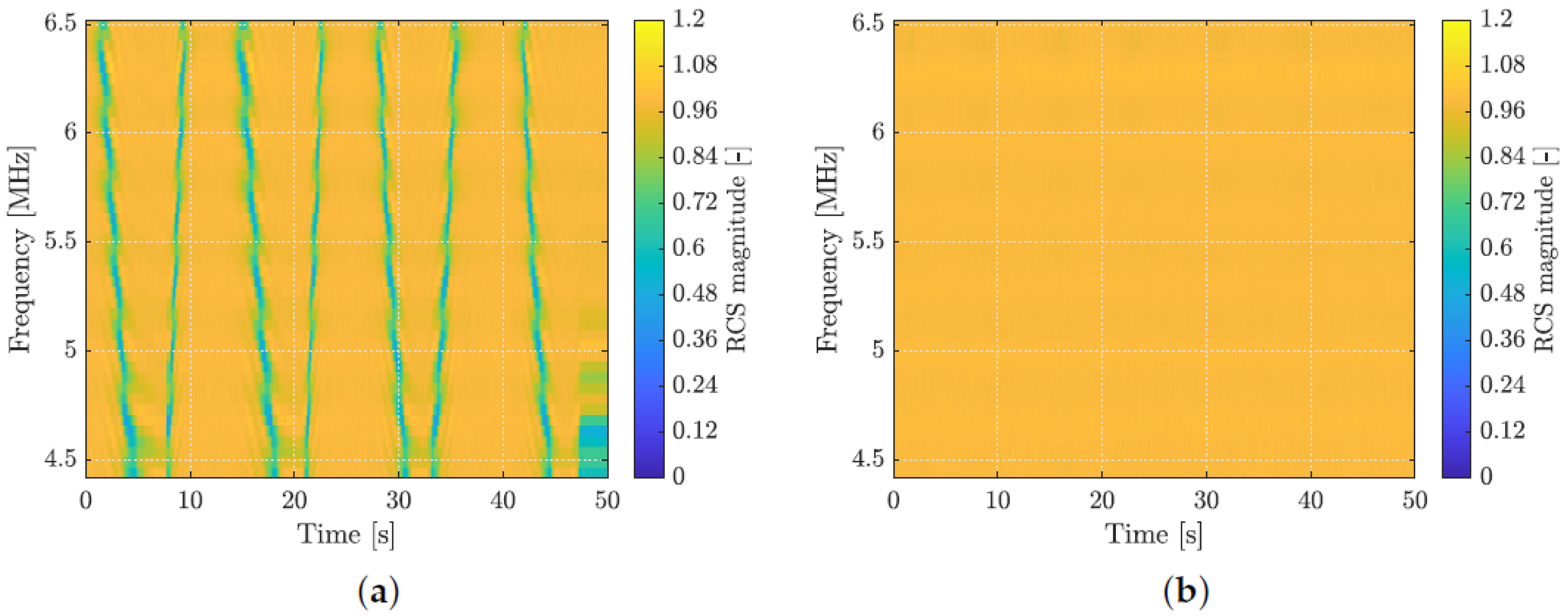
Figure 6 shows the spectrograms of the RCS calculated using the mean of the incident wave estimate found from manual calibration.
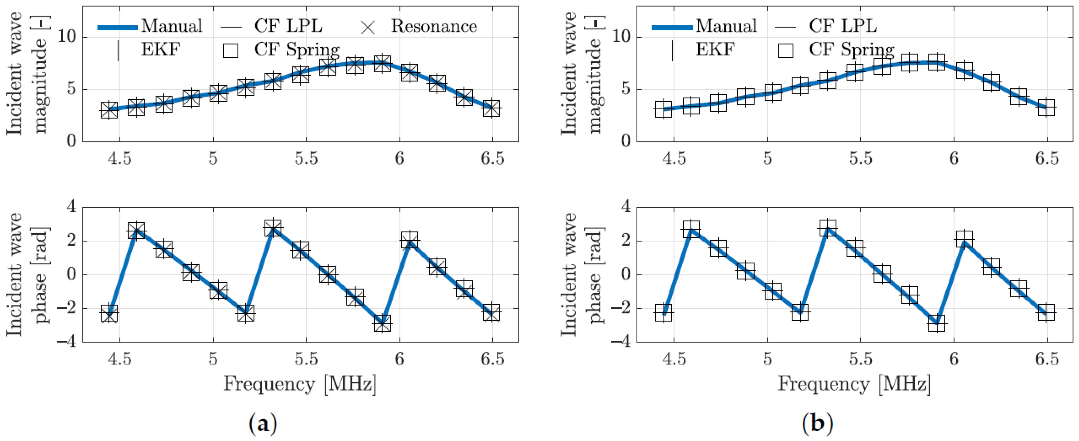
Figure 7 shows the magnitude and phase estimate of the incident wave using the discussed adaptive calibration methods. Notably, the figure shows the last instance of the EKF estimate, since this is continually updated. It is from the figure seen that all three adaptive calibration methods give very similar incident wave estimates. The figure further shows that these estimates closely resemble those found from manual calibration. This is also what is found in the studies describing the methods [
19,
21,
22].
Figure 8 shows the relative incident wave magnitude error and phase error. Notably, the phase error is shown instead of the relative error, due to the cyclic nature of the phase. It is seen that the resonance method, in general, has less error than both the curve fit and EKF method. However, the phase error of the resonance method has an approximately constant offset, whereas the other methods have a phase error that oscillates around the phase acquired from manual calibration. It is from the figure seen that the magnitude estimate error decreases, in the experiment where the resonance frequency is not detectable, compared to the other experiment, whereas the phase error is seen to be slightly increased.
To quantify the error in the incident wave estimate, the lubrication film thickness was calculated using the LPL lubrication film thickness estimation method, and the results are shown in
Figure 9. The LPL lubrication film thickness estimation method is outlined in [
15], and it was found to be a computationally efficient and accurate way of assessing the lubrication film thickness [
25]. Furthermore, the measurement of the change in lubrication film thickness from the laser is shown. Notably, the laser data are synchronised to the lubrication film thickness estimate found from the manual calibration data. It is also notable that the film thickness estimates shown are the average lubrication film thickness estimate across the frequencies. The figure shows that the deviations between the regression models are negligible. Furthermore, the deviation between the lubrication film thickness estimate achieved using manual calibration and the adaptive calibration resonance method is larger than the deviation from the other methods. The reason for the larger deviation might be because the resonance method has a constant offset in the phase, whereas the other method oscillates around the expected value. It is from
Figure 9a seen how the deviation and noise in film thickness estimates increase when the resonance frequency is not detectable. The deviation is also notable in
Figure 9b, where the film thickness estimate is seen to be offset from the manual calibration method by approximately 35 μm or
.
Figure 10 shows the LPL residual, Equation (
38), with the data from manual calibration, since this is a measure of the inaccuracies in the RCS model. It is by comparing
Figure 6 and
Figure 10 seen that the LPL regression model’s inaccuracy is at its peak at the resonance frequency. This is also evident when comparing the experiments shown in
Figure 10, where there is significantly less error in the experiment where the resonance frequency is not detectable.
Lastly,
Figure 11 shows the relative magnitude error of the EKF method to the manual calibration as a function of time and frequency.
Figure 11a shows how the error of the EKF algorithm peaks when the resonance frequency enters the transducer bandwidth and keeps being slightly larger than before the resonance frequency was detected. It is in
Figure 11b seen that the peak error is significantly less than in
Figure 11a, which is likely because the resonance frequency is not within the transducer bandwidth.
It is from these results seen that the EKF and curve fit methods give almost identical results after the EKF has converged. Furthermore, there is no distinguishable difference between LPL and spring model regression models when implemented with the curve fit method.
5.1. Sensitivity
It is from the lubrication film thickness estimates shown in
Figure 9 seen that the error between adaptive and manual calibration varies with thickness. The figure also shows how noise on the lubrication film thickness estimate varies. These tendencies were also found in the study by Dou et al. [
22]. The varying discrepancies and noise in the lubrication film thickness estimates can be explained by a sensitivity analysis of the lubrication film thickness. It is from Equation (
12) seen that the phase of the LPL is given by Equation (
50).
It is further seen that by isolating for
in Equation (
15), the
-product is given as in Equation (
51). This function is the foundation of the sensitivity analysis.
Equation (
51) describes the
-product and therefore also the lubrication film thickness as a function of both the magnitude and phase of RCS. The sensitivity analysis was for this reason split into two parts, analysing how a change in lubrication film thickness is described as a change in both RCS magnitude and phase. This is obtained from the partial derivative of
):
Lubrication film thickness sensitivity toward RCS magnitude, ;
Lubrication film thickness sensitivity toward RCS phase, .
Figure 12 shows the sensitivity of the lubrication film thickness to the magnitude and phase of the RCS as a function of the
-product. It is here seen that the lubrication film thickness is more sensitive to the phase error than the magnitude error, except when the lubrication film thickness is near the resonance frequency. This corresponds to the sensitivity analysis performed by Kaeseler and Johansen [
19]. Furthermore, the lubrication film thickness sensitivity to the phase is at its peak at
. This explains why the error and noise in the lubrication film thickness estimate are largest when the resonance frequency is not within the transducer bandwidth.
5.2. LPL Regression Model Inaccuracies
It is from
Figure 9a and
Figure 10a seen that even though the lubrication film thickness estimate deviation is smallest near the resonance frequency, the inaccuracy in the LPL regression model is at its peak at the resonance frequency. This discrepancy might originate from the assumption of
as assumed in the derivation of the LPL regression model. It is from Equation (
14) seen that this assumption corresponds to Equation (
52).
where
is a function of the times the ultrasonic pulse has been reflected in the lubrication film,
N in Equation (
14), within the time frame in which the reflected wave was measured. It is for the derivation of the LPL system representation assumed that this occurs an infinite amount of times. However, as mentioned in
Section 4, this assumption might not be valid when the resonance frequency is within the transducer bandwidth due to ringing.
Figure 13 shows an analysis of the magnitude of the lubrication layer spectrum evaluated at the resonance frequency as a function of the times reflected. It is from the figure seen how the magnitude of the lubrication layer spectrum exponentially converges to one, but is seen to deviate when the times reflected are low.
6. Regarding EKF Robustness and Reliability
It was in the study by Kaeseler and Johansen [
19] discussed how the EKF algorithm method has significant robustness and reliability problems. In the study, a robustness and reliability test was performed where the amplitude of the measured reflection wave was artificially reduced to
of the true value within a short time frame and afterwards restored to
. A similar test is seen in
Figure 14. In this test, the amplitude of the reflection wave was reduced to
between 20 s and 30 s. The figure shows how the EKF algorithm proposed by Kaeseler and Johansen [
19] at the start gives similar results as in
Figure 9b, but after the disturbance is introduced, it is seen to diverge and not be able to recover, even after the signal is restored. This robustness problem can be attributed to the structure of the proposed EKF algorithm. The update step of the EKF algorithm can be made to consist of some system process
and a process disturbance term
, as seen in Equation (
53).
where
is the noise term assumed to be Gaussian white noise with covariance matrix
. With this disturbance term included in the system model, the Kalman gain is calculated using Equation (
54).
where
is the covariance matrix of the predicted state instead of the corrected state, as in Equation (
39). The difference is that
entails the information about the disturbance, given by Equation (
55).
This also means that
is calculated using
instead of its previous value, as in Equation (
56).
The apparent problem with the EKF structure proposed by Kaeseler and Johansen [
19] is that the incident wave estimate is assumed to be a constant that should remain constant in time, similar to using all the data for a single curve fit. The benefit of this new EKF structure is that even though the incident wave estimate is still assumed to be a constant value, it is now allowed to update in time mostly relying on recent measurements, which is what is originally desired from the EKF algorithm. The results from this new EKF structure are seen in
Figure 14, where
is treated as a tuning parameter, chosen as Equation (
57).
Figure 14b shows that the new EKF structure converges to results similar to those obtained from manual calibration. It is from the figure also seen how all the lubrication film thickness estimates worsen during the period of reduced reflection wave amplitude, but both manual calibration and the new EKF structure recover after the signal is restored. Furthermore, the new EKF structure gives significantly better estimates than any other method, within the time frame of the manipulated signal. This is because the new EKF structure finds an incident wave estimate that does not correspond to the correct incident wave, but instead corresponds to that of the manipulated reflection wave signal. This corresponds to a better estimate of the RCS and, for this reason, also the lubrication film thickness.
Figure 14b also shows that the curve fit approaches give similar results independent of the regression model. It is seen that the curve fit approach underestimates the lubrication film thickness and has reduced dynamics. This is because the calibration using this method contains all measurements from the experiment, and the reduced signal has for this reason corrupted the data set. Notably, both the resonance method and curve fit approach are not prone to this error, if the calibration experiment is properly conducted.
7. Discussion
When comparing the methods, it is important to discuss the unique benefits and disadvantages. One disadvantage worth mentioning is the requirement of detecting the resonance frequency in the resonance adaptive calibration method. It is known from the resonance method for lubrication film thickness estimation that detecting the resonance frequency is not always possible, primarily due to the attenuation of the incident wave [
1,
15,
17]. It is from the definition of the resonance frequency, Equation (
44), seen that the resonance lubrication film thickness is given as in Equation (
58).
It is from Equation (
58) seen that if the lubrication layer is small, a large frequency is required. The problem is that the attenuation of acoustic waves is a function of frequency, and the relationship is often in the order of
or larger ([
18], pp. 386–390). This means that there is a practical limit to how large the detectable resonance frequency is before the penetration depth of the ultrasonic wave becomes too short to be applied in industrial applications. This has been a limiting factor for the lubrication film thickness estimation resonance method and potentially is a limiting factor of the adaptive calibration resonance method, where this limits the use of the method to fairly thick lubrication films.
One of the great benefits of the method proposed by Kaeseler and Johansen [
19] is the use of EKFs for continuous in situ adaptive calibration, which is a property the other methods lack. However, as discussed in
Section 6, further research on the EKF structure seems beneficial to address the problems outlined by Kaeseler and Johansen [
19]. One such reconfiguration is referred to as a tribodynamic state observer (TSO). A TSO aims to expand upon the EKF, to include a model of the lubrication film thickness dynamics and information about the system inputs. This could for example be developed for systems such as journal bearings since dynamic models for journal bearings are well established. The challenges of the TSOs are simplifying the dynamic models to be implemented into an EKF structure with the ultrasound measurements.
A TSO approach was attempted by Nielsen et al. [
26], and the results from this study showed through simulation that TSOs potentially not only aid in the accuracy, precision, and robustness of the incident wave/lubrication film thickness estimate, but also allow for the estimation of other system parameters affecting the tribodynamics of the system, such as lubrication film viscosity. However, these results lack experimental validation, and further investigation into the TSOs is for this reason needed. The disadvantage of the TSOs is the need for dynamic system models. Because of this, TSOs are limited to specific systems and are less general than the adaptive calibration methods discussed in this paper.
The experimental data used in this study only contain reflection wave measurements from a thick lubrication regime. These data might be sufficient in comparing the methods. However, it does not show any modelling errors that might occur when the lubrication film thickness is reduced to a mixed or boundary lubrication regime, which might affect all three methods discussed in this paper. Furthermore, the methods are also prone to modelling errors in the assumed three-layered structure model. This includes the assumption that the solid layers are parallel to each other, that there only are three layers, attenuation in the lubrication layer is negligible, and any uncertainty in the acoustic parameters, such as the reflection coefficients and especially any error in the speed of sound in the lubrication layer. Both the density and speed of sound in the materials are temperature dependent. This means that temperature changes affect the accuracy of the regression models or, for the case of the adaptive calibration resonance method, the lubrication film thickness calculation, Equation (
46). It is for these reasons of great interest to further investigate and improve upon the adaptive calibration methods, such that they are robust towards these errors. A recent study by Jia et al. [
27] found that the most critical factors regarding temperature changes are changes to the incident wave and changes to the acoustic parameters of the lubrication layer. The changes to the incident wave are solved by adaptive calibration, and in the study, it was addressed how it is possible to compensate for temperature changes through predetermined experimental material property regression models. These models also have the potential to be used in a TSO setting where it might be possible to estimate the temperature in the lubrication layer locally and, for this reason, also the material properties.
8. Conclusions
In this paper, three different methods of performing adaptive calibration for ultrasound reflectometry in lubrication layers were compared. Two of the three methods compared were the curve fitting and the extended Kalman filter approach, which both rely on fitting parameters from regression models. The two studies where these methods were proposed presented the use of two different regression models. The regression models were in this paper compared, and based on experimental data and theoretical analysis, it was found that for many practical purposes, the differences between the regression models are negligible. However, it was also found that the spring-model-based regression model is less general and yields little to no advantages concerning model simplicity when compared to the layer-phase-lag-based regression model. The spring-model-based regression model was from this comparison for this reason found to be redundant.
This paper also compared both the curve fitting and the extended Kalman filter approach for the layer-phase-lag-based regression model. The comparison was based on results from experimental testing. Here, it was found that as originally proposed, both methods gave very similar results. However, the extended Kalman filter approach allows for continuous in situ calibration and was for this reason found to be of great interest. It was in this paper also showed how a restructuring of the extended Kalman filter algorithm can compensate for some of the original concerns regarding robustness and reliability.
A third method of performing adaptive calibration was also compared. This method was an algorithm based on the detection of the system resonance frequency and, from this, the recreation of the incident wave spectrum. This method was found to yield similar to slightly better results than the other two methods compared in this paper. However, this method was found to be limited to relatively thick lubrication films, due to the requirement of detecting the resonance frequency. Due to this and because it is not continuously updatable, it was found to not have the same potential as the extended Kalman filter approach.
The comparison of the methods was based on data found from a thick lubrication film. This is believed to be sufficient for the comparison of the methods, but did not show any modelling error when this was not the case. It was from this study found that continuous in situ adaptive calibration methods such as an extended Kalman filter approach show the greatest potential, but further research into the robustness and reliability of acoustic modelling errors for all the methods is still needed.


