Article

A Rolling Horizon Optimization Framework for Resilient Restoration of Active Distribution Systems

1
College of Water Resources and Electric Power, Qinghai University, Xining 810016, China
2
Qinghai Key Laboratory of Efficient Utilization of Clean Energy, Tus-Institute for Renewable Energy, Qinghai University, Xining 810016, China
*
Author to whom correspondence should be addressed.
Energies 2022, 15(9), 3096; https://doi.org/10.3390/en15093096
Submission received: 24 March 2022 / Revised: 17 April 2022 / Accepted: 22 April 2022 / Published: 24 April 2022

Abstract

:
Network reconfiguration is an effective way to avoid severe, large-scale power outages and to improve the resilience of active distribution networks (ADNs). Furthermore, the rapid development of distributed energy resources (DERs) provides new perspectives for network reconfiguration. In this paper, the effect of network reconfiguration and DER collaboration on ADN’s resilient restoration are studied. The applications of DERs are fully explored. In order to achieve a better resilient performance, a detailed multiperiod model considering both reconfiguration and multiple DERs is established. Some linearization techniques are used to simplify the proposed model. Then, we build a rolling horizon optimization framework to solve the model. The framework eliminates the adverse effect of prediction errors and speeds up the calculation. By introducing predictions into strategy determination, the framework achieves a better restoration effect than the traditional greedy method. The proposed framework is tested on a 33-bus system. The simulations verify the efficiency of our work.

Graphical Abstract

1. Introduction

Recently, distributed energy resources (DERs), including energies of solar and wind, have been widely integrated into active distribution networks (ADNs) to avoid infrastructure costs, improve resilience, and achieve low carbon emissions [1]. However, most DERs are renewable energies, with a high degree of uncertainty and volatility. Their applications may cause significant negative impacts on ADN’s operations.
Many technologies are being developed to deal with the problems caused by the DER penetrations. Network reconfiguration attracts much attention due to its ability to optimize operations by adjusting the system’s topology [2]. With advanced dispatchable switches equipped in the ADN, the network can be changed flexibly to improve the operation quality and eliminate the preceding effects. At present, there is some research on the reconfiguration of the ADN. It has been already used in supporting voltage/frequency control [3], energy management [4,5], and power outage recovery [6], etc.
In recent years, urban power grids have been facing the threats of extreme disasters. Many scholars have noticed that the network reconfiguration can realize a regional power supply of damaged grids. Therefore, it has also been widely applied in the field of system resilience enhancement.
Ref. [7] established a basic reconfiguration model for ADNs equipped with a complex communication system. An improved consensus algorithm is proposed to realize the joint restoration for both systems. Ref. [8] designed a leader–follower control structure and used the mixed-integer second-order cone programming to speed up the solution. Ref. [9] formed a two-stage optimization considering the uncertainties before and after a disaster. Ref. [10] studied the deployment strategy of remote switches to support further control when facing an emerging situation. Ref. [11] invented an identification method for critical switches based on network reconfiguration by forming a two-stage robust optimization. Ref. [12] applied multiagent soft actor–critic techniques on the reconfiguration of AC/DC hybrid distribution networks to obtain better resilient performances.
As mentioned above, most of the research is focused on the system topology techniques. Combined with local energy storage and diesel generators, these methods can achieve rapid system recovery. Recently, the development of different energy forms has provided more new insights [13]. Renewable energy is the first concern. The control problem of wind turbines for network reconfiguration is analyzed in [14]. Ref. [15] further considered photovoltaic sources in the system emergency operation. Ref. [16] designed a resilient control strategy based on a power router with renewable generation and network reconfiguration.
Mobile power sources have been introduced for resilient restoration. Ref. [17] combines the mobile power sources and logistics resources to coordinate with the network reconfiguration. Ref. [18] explored the potential of mobile sources on seismic resilience of ADN. Transportation-electrification techniques can also improve a system’s resilience. Ref. [19] designed a resilience-based architecture for joint distributed electric vehicles allocation and hourly network reconfiguration. The feasibility of electric buses is discovered. The preallocation [20] and post-disaster restoration [21] of electric buses were studied, respectively.
In this work, we will focus on the resilient application of network reconfiguration with multiple power sources. However, there still exist some research gaps, as follows:
  • An ADN consists of more than one type of power source which can serve as an emergency backup generator. The restoration problem considering network reconfiguration still needs to be modeled in more detail.
  • The multiperiod restoration problem needs lots of predictions, which introducing prediction errors into the model. Additionally, the existence of a large number of integral variables will limit its application.
In this work, we match the DERs and network reconfiguration to help the system enhance its resilience. The key contributions of this work are twofold:
  • We establish a detailed multiperiod resilient network reconfiguration model, which considers different power supply sources (including DERs). The impacts of network changes on power flow and voltage are fully studied. In addition, some linearization techniques are adopted to reduce the complexity of the model.
  • We develop a rolling-horizon-optimization-based framework for this multiperiod problem in order to make effective use of predictions and speed up the model computation. This method can reliably solve the reconfiguration problem.
In the following, Section 2 establishes a detailed model for the resilient network reconfiguration in coordination with multiple sources. Section 3 proposes a rolling horizon optimization framework to deal with the existence of prediction errors and low computational speed. Section 4 gives the numerical results. Section 5 concludes the work.

2. Multiperiod Network Restoration of Distribution Systems
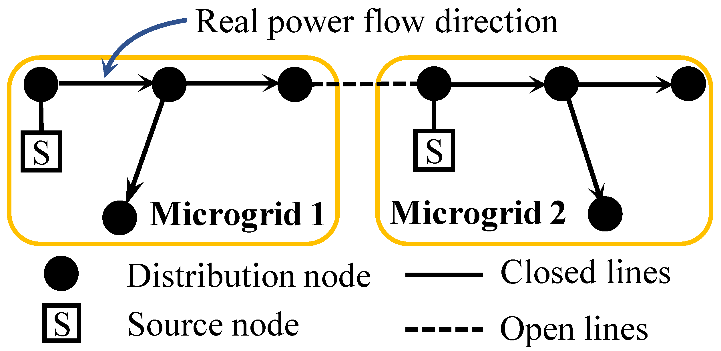
2.1. Preliminaries

The distribution network is always modeled as a connected undirected graph G = N , L , where N is the set of distribution nodes, and L is the set of all distribution lines. The set N S is defined to represent the power source nodes, including feeders, DERs, and energy storage systems (ESSs). In daily operation, the topology of the distribution network should maintain a radial structure in order to facilitate coordinations and protections.
When facing extreme events (e.g., earthquake, wildfire, meteorological disasters), large-scale power outages may happen due to the distribution line damages. The network reconfiguration problem aims to minimize the potential power losses by adjusting the topology with intact equipment. The entire network may be divided into several disconnected microgrids (MGs), and then the loads are powered by different sources in MGs according to their priorities.
In the reconfiguration process, if we still use an undirected graph to model the distribution network with a radial structure, a phenomenon of “pseudo-root” may occur and influence the resilient effect [22]. Thus, in this work, we apply the theory of directed spanning trees on modeling to realize a better restoration and avoid the mentioned problems. An illustration of applied theory on the DS is given in Figure 1.
In this figure, the arrows indicate the parent–child relationships between two adjacent nodes. The reconfigured MGs are modeled as several spanning trees. Each distribution node is assigned with one virtual unit demand. In addition, source nodes are treated as the roots of different MGs and are the only sources of virtual demands. By defining the virtual demands and sources, the connectivity and the radial structures of MGs can be strictly guaranteed. Furthermore, we can further model the reconfiguration model and determine the actual directions of power flows with these concepts.

2.2. Radiality Constraints

Maintaining the radiality of MGs should first be met in the resilient restoration. With the predefined virtual demands ( F i , t L = 1 ), we have the following constraints.
s i j , t u i j , t , ( i j ) L
s i j , t = s i j , t d + s j i , t r , ( i j ) L
s j i , t r = 0 , s i j , t d = 1 , j N S
z k , t i S ( k ) s i k , t d + j S ( k ) s j k , t r 1 , k N
| z i , t z j , t | 1 s i j , t , i , j N
z i , t F i , t L = j S ( i ) F i j , t , i N
| F i j , t | s i j , t | N | , ( i j ) L
where u i j , t { 0 , 1 } reflects the impacts of extreme events on the distribution lines. Since distribution lines are often exposed to the outdoors, they are vulnerable to extreme events, such as hurricanes and wildfires, etc. When extreme events damage the line ( i j ) at t, we set u i j , t = 1 ; and when the extreme events do not cause damage to the line (i.e., the line is intact), we set u i j , t = 0 . s i j , t { 0 , 1 } indicates the line states. s i j , t d , s j i , t r { 0 , 1 } are two auxiliary variables representing the power flow directions. z k , t { 0 , 1 } represents the power supply states of distribution nodes. F i j , t represents virtual power flow on line ( i j ) . | N | is the cardinality of set N . S ( k ) is the set of nodes connecting to node k.
Constraint (1) states that the line states are restricted by the equipment states. Constraint (2) indicates that the power flow on each line has only one direction. Constraint (3) expresses the root nodes only have out degree in the spanning tree (since they are the source node of the virtual demands). Constraint (4) reflects the parent–child relationships. Constraint (5) is the consistency constraint of line states and nodes states (on both sides). Constraints (6) and (7) restrict the flow of virtual demands, exhibit the conservative of the virtual flow, and guarantees the radiality structure.

2.3. Power Flow Constraints

The control and adjustment of the network topology will affect the power flow of the ADN. In this section, we analyze the relations between reconfiguration and system operation, then we give a detailed model.

2.3.1. Power Balance

In this work, we adopt the LinDistFlow [23] model to describe the power flow conversation, which is listed as follows.
( i j ) L P i j , t = P i , t G P i , t L , i N , t
( i j ) L Q i j , t = Q i , t G Q i , t L , i N , t
0 P i , t L z i , t · P i , t L , max , i N , t
Q i , t L = tan cos 1 ϕ i P i , t L , i N , t
P i , t L P i , t + 1 L , i N , t
( P i j , t ) 2 + ( Q i j , t ) 2 s i j , t · ( S i j max ) 2 , ( i j ) L , t
where P i j , t , Q i j , t are the active/reactive power flow on distribution line ( i j ) at time t. P i , t G , Q i , t G are the power output generation at node i. P i , t L , Q i , t L represent the active/reactive load demands at node i. ϕ i is the power factor of load i.
Constraints (8) and (9) represent the active/reactive power flow balance on each line and node. Constraints (10) and (11) reflect the range of restored loads. Constraint (12) indicates that the picked-up loads will not be shut down again. Constraint (13) is the line capacity constraints of each distribution line ( i j ) .

2.3.2. Voltage Constraints

Except for the power-flow-related constraints, the change of nodal voltages should also be considered. Therefore, we have the following constraints:
v i t v j t M 1 s i j , t + R i j P i j t + X i j Q i j t V 0 , ( i j ) , t
v i t v j t M s i j , t 1 + R i j P i j t + X i j Q i j t V 0 , ( i j ) , t
v i t = V 0 , i N S , t
z i , t v i min v i t z i , t v i max , i N N S , t
where v i t is the voltage magnitude of node i at time t. R i j and X i j are the resistance and reactance of the line ( i j ) , respectively. M is a large enough positive number. V 0 is the reference value of nodal voltage. v i min and v i max are the lower/upper bounds of voltages, respectively.
Constraints (14) and (15) reflect the relationships between nodal voltages and power flows. The big-M theory is applied to ensure that there is a correct relationship between the two under the influences of line states. To better illustrate the use of M and the meaning of Constraints (14) and (15), we have the following discussion.
When s i j , t = 1 , Constraints (14) and (15) can be transferred as:
v i t v j t = R i j P i j t + X i j Q i j t V 0 , ( i j ) , t
Thus, we can see that the voltage relationship between two adjacent nodes can be guaranteed. However, when there is a line disconnection between these two nodes (i.e., s i j , t = 0 ), the equation no longer exists. There is no deterministic relationship between v i t and v j t . Then, Constraints (14) and (15) can be transferred as:
v i t v j t M + R i j P i j t + X i j Q i j t V 0 , ( i j ) , t v i t v j t M + R i j P i j t + X i j Q i j t V 0 , ( i j ) , t
When M is large enough, R i j P i j t + X i j Q i j t V 0 can be neglected, while Constraints (14) and (15) are relaxed. That is, M v i t v j t M .
Constraint (16) sets the voltages of root nodes. Constraint (17) sets the voltage range for the rest of the nodes. With all these constraints, the power quality can still maintain at a high level when facing extreme events.

2.3.3. Power Outputs

In this section, we study the sources of possible power supplies and their operation characteristics. These sources cooperate with each other to achieve fast power supply in the outage areas.
  • Feeders: The feeders are the main source of power supply. For each nodes connecting to the main grid, we have the following constraints:
    P i , t G , min P i , t G P i , t G , max , i N F , t
    Q i , t G , min Q i , t G Q i , t G , max , i N F , t
    where N F is the set of feeders. P i , t G , min and P i , t G , max are the lower and upper bound of the active power supply at the feeder, respectively; Q i , t G , min and Q i , t G , max are the lower and upper bound of the reactive power supply at the feeder, respectively. P i , t G , min and Q i , t G , min can be positive or negative.
  • DER outputs: With the development of DERs, different forms of energies, such as wind and solar, are integrated into the ADNs. In the post-event restoration, these types of DERs can realize an emergency power supply through equipped smart inverters. Their output ranges are:
    P i , t DER , min P i , t G P i , t DER , max , i N DER , t
    Q i , t DER , min Q i , t G Q i , t DER , max , i N DER , t
    where N DER is the set of nodes equipped with DERs. In this work, we focus on renewable energies. Their output ranges can be obtained with accurate predictions.
    It is noted that the damaged ADN in our work is separated into several islanded MGs to realize an emergency power supply with DERs and storage. Under this circumstance, the DERs should be operated in a Volt-Var (QV) response mode since the islanded MGs lack reactive power support. The DERs operating in QV mode can maintain the voltage and distribution of active power by outputting reactive power. As line repair progresses, DERs can switch their control strategy since the islanded MGs are reconnected to the main grid. The system can obtain the reactive power from the grid. Thus, DERs could choose strategies such as “Maximum Power Point Tracking”, etc., to output more active power.
  • ESS outputs: The ESS can keep the ADN in balance. Considering the process of charging and discharging, we have the following constraints for the nodes ( i N ES ) equipped with ESS:
    P i , t G = P i , t dch ( 1 s i ES ) P i , t ch , i N ES , t
    where N ES is the set of nodes equipped with ESS; P i , t dch is the power discharged from the ESS to the ADN; P i , t ch is the power that the ESS can charge from the ADN. The difference between P i , t dch and P i , t ch calculated in Constraint (22) determines the power that the ESS feeds into the system.
  • Pure load nodes: As for pure load nodes, they cannot feed power back to the grid. Hence, we set P i , t G and Q i , t G as:
    P i , t G = 0 , i N N S , t
    Q i , t G = 0 , i N N S , t

2.3.4. Power Load Model

Except for the power generation, it is also essential to give a detailed model for power loads since they are always voltage-dependent. Static analyses often use ZIP load models, which consist of constant impedance (“Z”), constant current (“I”), and constant power (“P”) components.
The ZIP loads can be expressed as:
P i , t L = a 1 i ( v i t ) 2 + a 2 i v i t + a 3 i
Q i , t L = b 1 i ( v i t ) 2 + b 2 i v i t + b 3 i
In Constraints (25) and (26), a 1 i , a 2 i , a 3 i and b 1 i , b 2 i , b 3 i are scalar parameters, where:
  • a 1 i and b 1 i specify the constant impedance for active and reactive power demands on bus i.
  • a 2 i and b 2 i specify the constant current for active and reactive power demands on bus i.
  • a 3 i and b 3 i specify the constant power for active and reactive power demands on bus i.
In this work, we mainly focus on the restoration effect of the network reconfiguration and DER operation. For simplicity, we just consider the constant power in the ZIP model for the following simulations.

2.3.5. Ess Operation

In addition to the damaged ADN, the operation ESS should also be concerned. For ESS connecting on node i N ES , we have:
S O C i , t + 1 = S O C i , t + P i , t ch η i ch P i , t dch η i dch , i N ES , t
where η i ch / η i dch are charge/discharge efficiency. S O C i , t is the state-of-charge (SOC) of ESS i at time t.
Since an ESS can only operate at charging state or discharging state, we define a binary variable s i , t ES to represent the state of the ESS. When s i , t ES = 1 , the ESS works in a discharging state; when s i , t ES = 0 , vice versa. Constraints (28) and (29) restrict the output range of discharging and charging power of the ESS.
0 P i , t dch s i , t ES P i , t dch , max , i N ES
0 P i , t ch ( 1 s i , t ES ) P i , t ch , max , i N ES
It is noteworthy that the excessive charging and discharging of the ESS during the restoration process may affect the lifetime of the ESS. In order to prolong and preserve its lifetime, we can restrict the total charging/discharging power and the number of state transitions. Hence, we have the following constraints:
t = 1 T | P i , t ch | + | P i , t dch | P L T max , i N ES
t = 1 T 1 | s i , t + 1 ES s i , t ES | N i max , i N ES
where P L T max is the maximum allowable operating power for a period of time T R ; N i max is the maximum number of allowable state transitions in a period of time T R ; T R could be a predefined finite horizon.
In this work, we focus on the restoration effect of DERs and network reconfiguration. The operation of ESSs is regarded as an assistant measurement. We will consider the impact of the restoration process on the lifetime of the ESS in our future work.

2.4. Linearization Technique

We notice that there are quadratic terms (i.e., ( P i j , t ) 2 and ( Q i j , t ) 2 ) in our model. Constraint (13) has strong nonlinearity, restricting the model solution. Thus, before forming the complete multiperiod optimization model, we linearize the constraints to reduce the computational efficiency.
In this work, the following two constraints are used to approximately substitute Constraint (13):
s i j , t · S i j max P i j , t , Q i j , t s i j , t · S i j max
2 s i j , t · S i j max P i j , t , Q i j , t 2 s i j , t · S i j max
The feasible region of the decision variables P i j , t and Q i j , t exhibits in the shaded area of Figure 2. It can be seen that we use polygon to approximate the feasible circular region. This technique transforms the problem into a linear form, which relieves the computational burden greatly.
However, we need to point out that this linearization technique may have potential risks since the line capacity constraints may be violated during operation. To deal with this problem, more polygons can be used to realize an accurate approximation of the line capacity constraints. In engineering applications, it is acceptable to use two rectangular regions to approximate this constraint. Later, we further discuss the possible effects that this linearization may cause.

2.5. Multiperiod Reconfiguration Model

After modeling the post-event system operation, we can finally build the optimization model. This model aims to reduce the extreme event-induced load losses, which can be written as:
min t ω i ( P i , t L , max P i , t L ) Δ t
where ω i is the load value of node i. P i , t L , max is the load forecast. Δ t is the time period. The objective function can determine the total load losses by computing the difference between the predicted loads and the real supplied loads.
With the preceding constraints, we have the following complete model:
  • Objective function: (34)
  • Network reconfiguration: (1)∼(7)
  • Power system operation: (8)∼(12), (32) and (33), (27)
  • Voltage constraints: (14)∼(17)
  • Power output: (18)∼(24)
Remark 1.
Unmentioned parameters are boundary parameters of corresponding variables.
The established multiperiod optimization model is a mixed-integer linear programming (MILP) problem. In solving this model, a large number of integer variables are involved. Furthermore, load predictions are required at the same time. The existence of prediction errors will make the solutions deviate from the optimum. In order to further speed up the solution and eliminate the adverse effects of prediction errors on the strategy, we design a rolling-horizon-optimization-based framework.

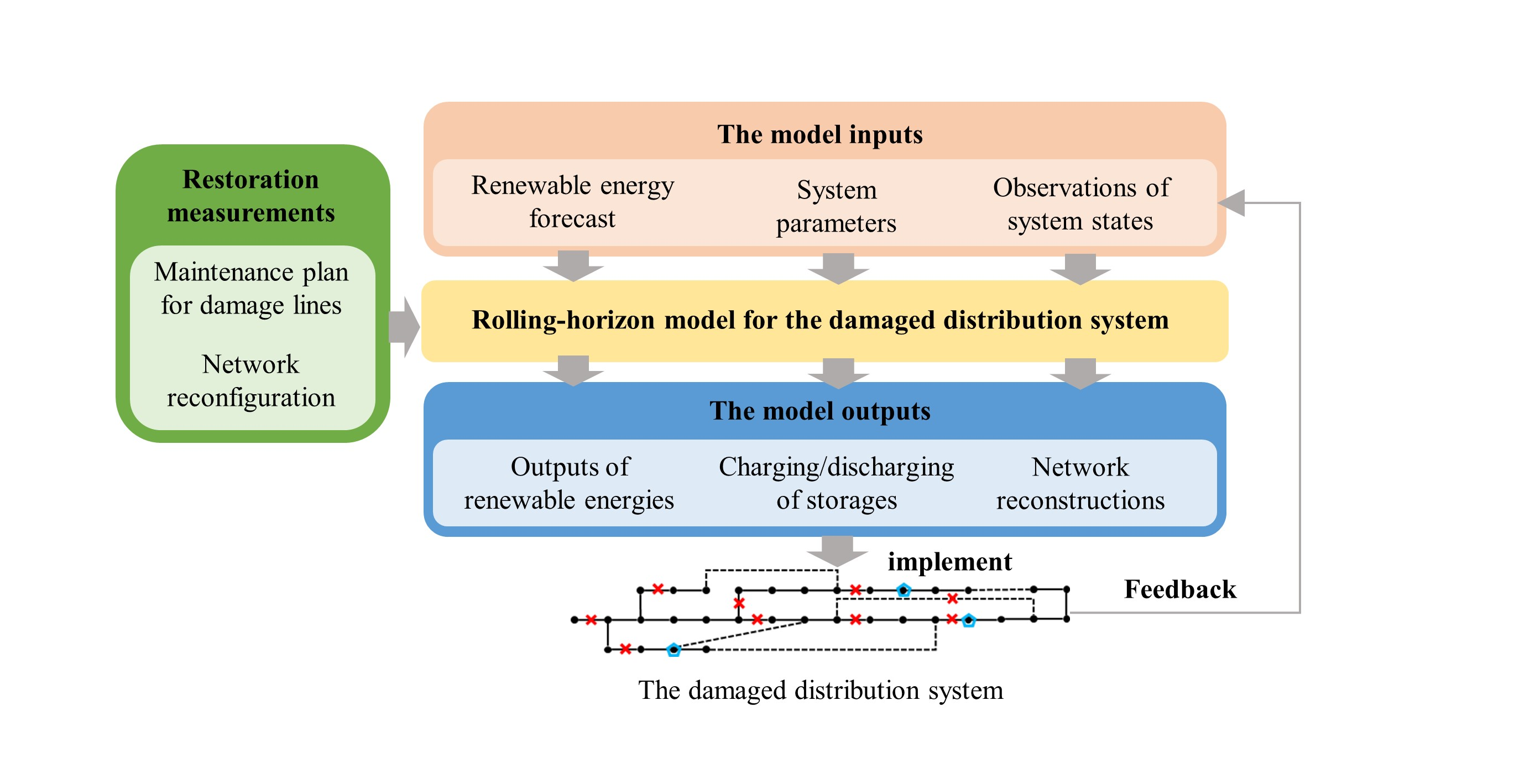
3. Rolling Horizon Optimization Framework for Resilient Restoration

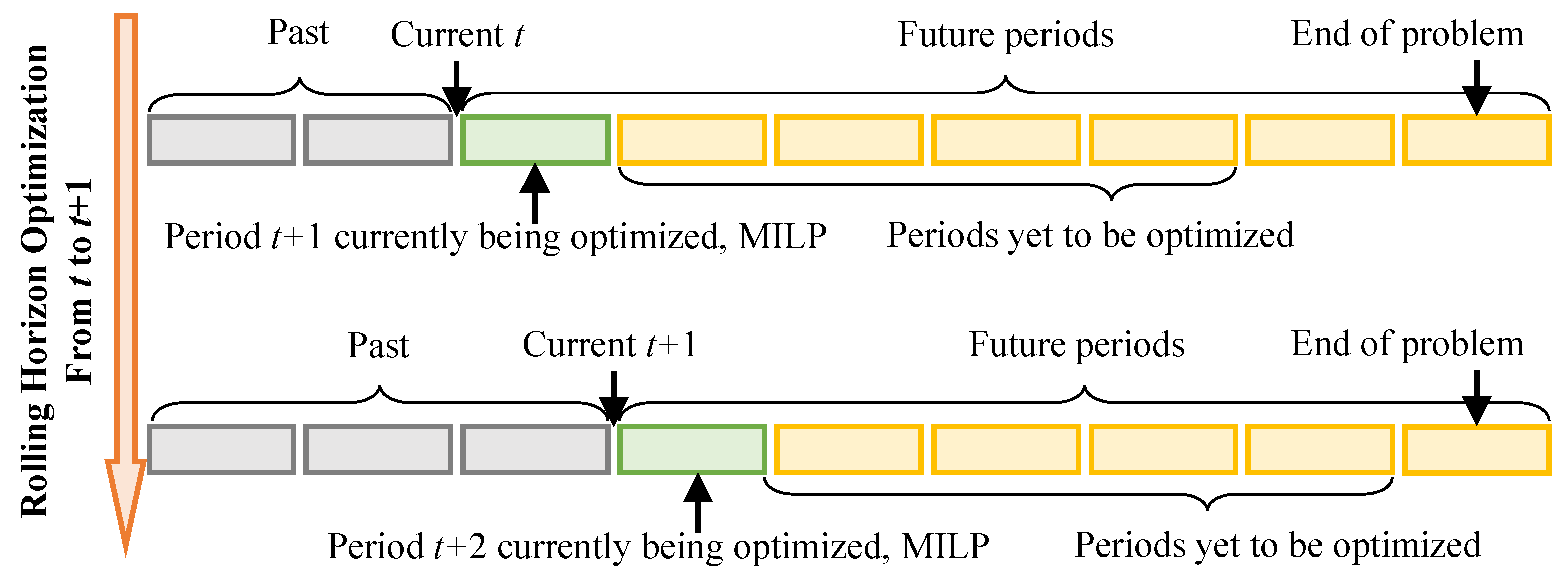
3.1. Basics of Rolling Horizon Optimization

The rolling horizon heuristic optimization is an advanced method to control a multiperiod process [24]. Its advantage is that it allows optimizing the operation in the current period while considering the future periods simultaneously. This achieves by optimizing a finite horizon but only implementing the current period. The above optimization will be repeated until the end of the problem.
Rolling horizon optimization can continuously obtain the latest predictions to update the current control strategy, so it can reduce the impact of prediction errors on the optimality of control. In addition, it only solves a finite-horizon optimization problem, which reduces the problem scale greatly.
Take the model we studied as an example. The established model is the MILP problem. Assuming that the restoration process lasts for T, the model will contain 4 × | L | + | N | integral decision variables, which tends to be a lot. However, if we only consider the optimization problem of finite time T L , the number of integral variables that need to be solved will become T L T of the original. In Figure 3, we give the framework of rolling horizon optimization.

3.2. Steps of Solving Restoration Strategy with Proposed Methods

With Figure 3, we can give the detailed solution steps for the resilient network restoration. Let us assume that we are at the end of the t-th period, so the states of the system, including SOC of storage and line states over the past period 1, ⋯, t 1 are already known. With this information, we aim to determine the network reconfiguration and system operation strategy for future periods.
  • Step 1: Update predictions of user’s load, DER outputs from t to t + t L ; update SOC of storage and the line states with line maintenance plan over 0 to t 1 .
  • Step 2: Solve the optimization problem established in Section 2.5 with updated predictions.
  • Step 3: Apply the solved operation strategy at period t; record the system states at the beginning of period t + 1 .

4. Case Study

The case study is performed on a modified 33-bus system [25] to validate the effectiveness of the proposed resilient network restoration problem and the rolling horizon optimization framework. Our research is implemented using C++ 11 and solved by CPLEX 12.80. Our testbed is a personal computer with an Intel Core 2.5 Hz processor and 16 GB memory. The MIP gap is set as 0.1%.

4.1. System Parameters

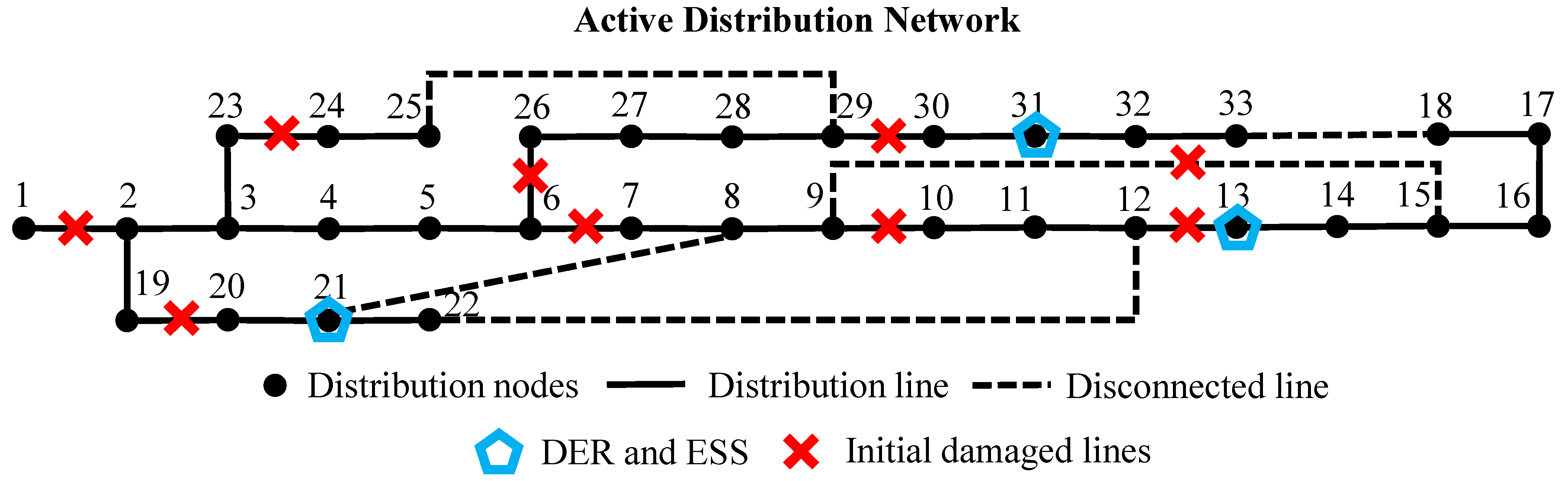
4.1.1. System Configurations

The test system contains three DERs and three ESSs, which are located at bus #13, #21, and #31. The situation of line damages is shown in Figure 4. Because the repair process is quite essential in the restoration process, we set a maintenance schedule for each damaged line. The schedule is shown in Table 1, which is from [25].

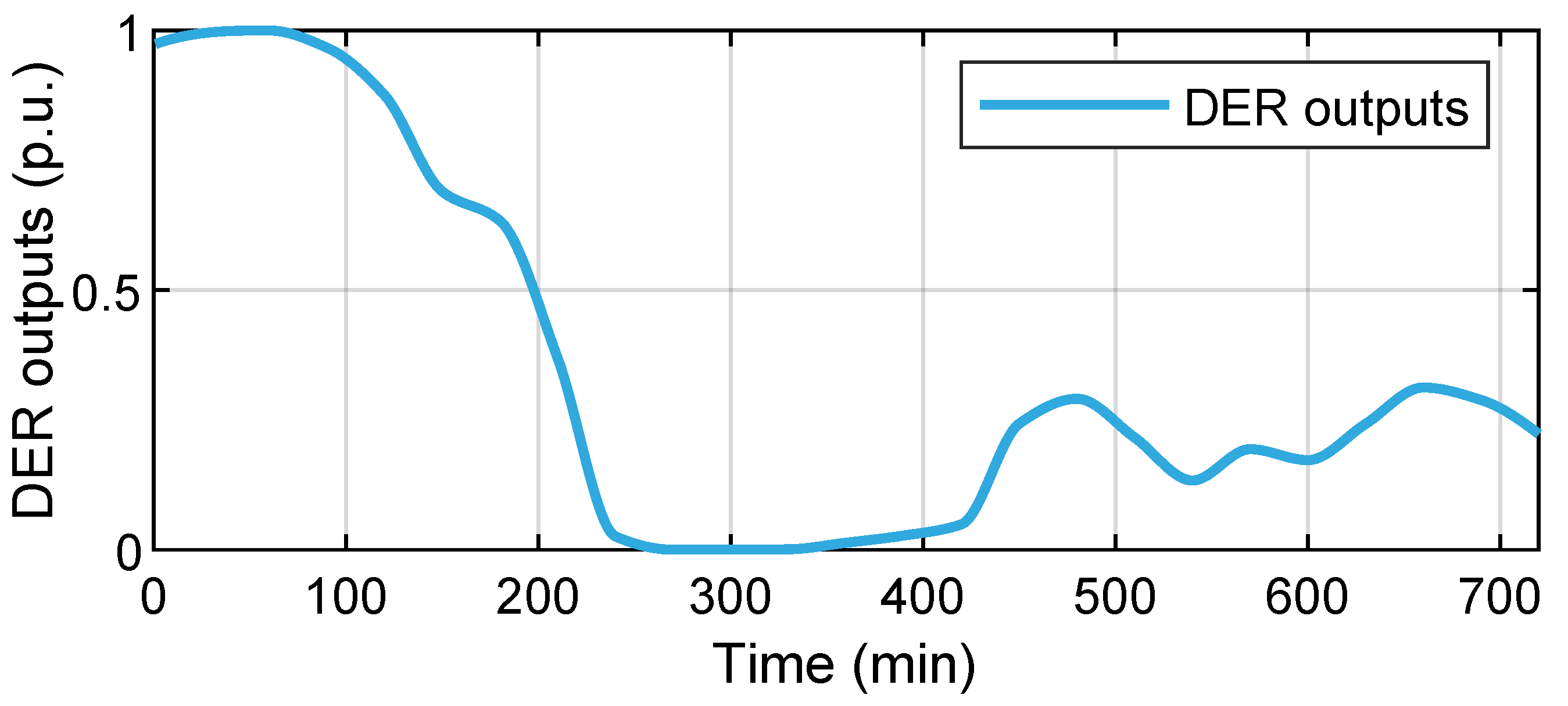
4.1.2. Predictions of Loads and DER Outputs

In this case, the restoration process is supposed to last for 12 h (from 6:00 a.m. to 6:00 p.m.). Considering that the DERs are applied to raise the resilience level of the system and try to help recover the outage loads, we use the following curves in Figure 5 and Figure 6 that reflect the load and DER fluctuations. The time interval is set as 15 min. In this case, we use five periods of forward predictions to solve the rolling horizon optimizations.
The curve inferred that DERs are important to the ADN that is disconnected from the main grid. However, the high intermittent limits their applications.

4.2. Restoration Effect

4.2.1. The Process of Network Reconfiguration

At first, we exhibit the change of network reconfiguration in the whole process. During restoration, the number of disconnected lines fluctuates in the range of [ 8 , 18 ] .
The reconfiguration process is in coordination with the output of renewable energies, which realizes a high-speed restoration. The damaged ADN is split into different areas with remote switches and is powered by the DERs.

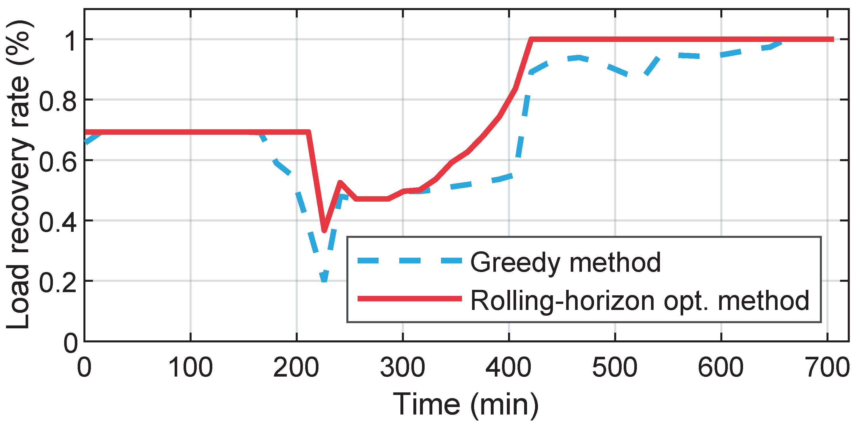
4.2.2. Restoration Effect of Proposed Method

We compare the restoration effect of ADN with greedy and proposed methods. The former one (greedy method) is a simple, intuitive method that is widely used in optimization. This method determines the optimal decisions at each period. Then, it tries to explore the overall optimal way of the entire problem.
In Figure 7, comparing two methods, the rolling horizon method can restore more outage loads than the greedy method. The former can achieve full load recovery earlier than the latter. This is because more energy is stored in ESS with a control strategy obtained by the rolling horizon optimization. We find that when t [ 166 , 405 ] , the load recovery rate has decreased since the DER outputs turn to 0. However, with the existence of ESSs, the disconnected ADN can still maintain a certain load recovery rate.
Furthermore, we can figure out from Figure 7 that the load restoration curve obtained by the proposed method is smoother, thereby avoiding the violent interruptions and fluctuations of loads during the recovery process.
The reason for this phenomenon is that the predictions of loads and DERs’ outputs are neglected, while the rolling horizon methods introduce the future information into current decisions, thus having a better performance.

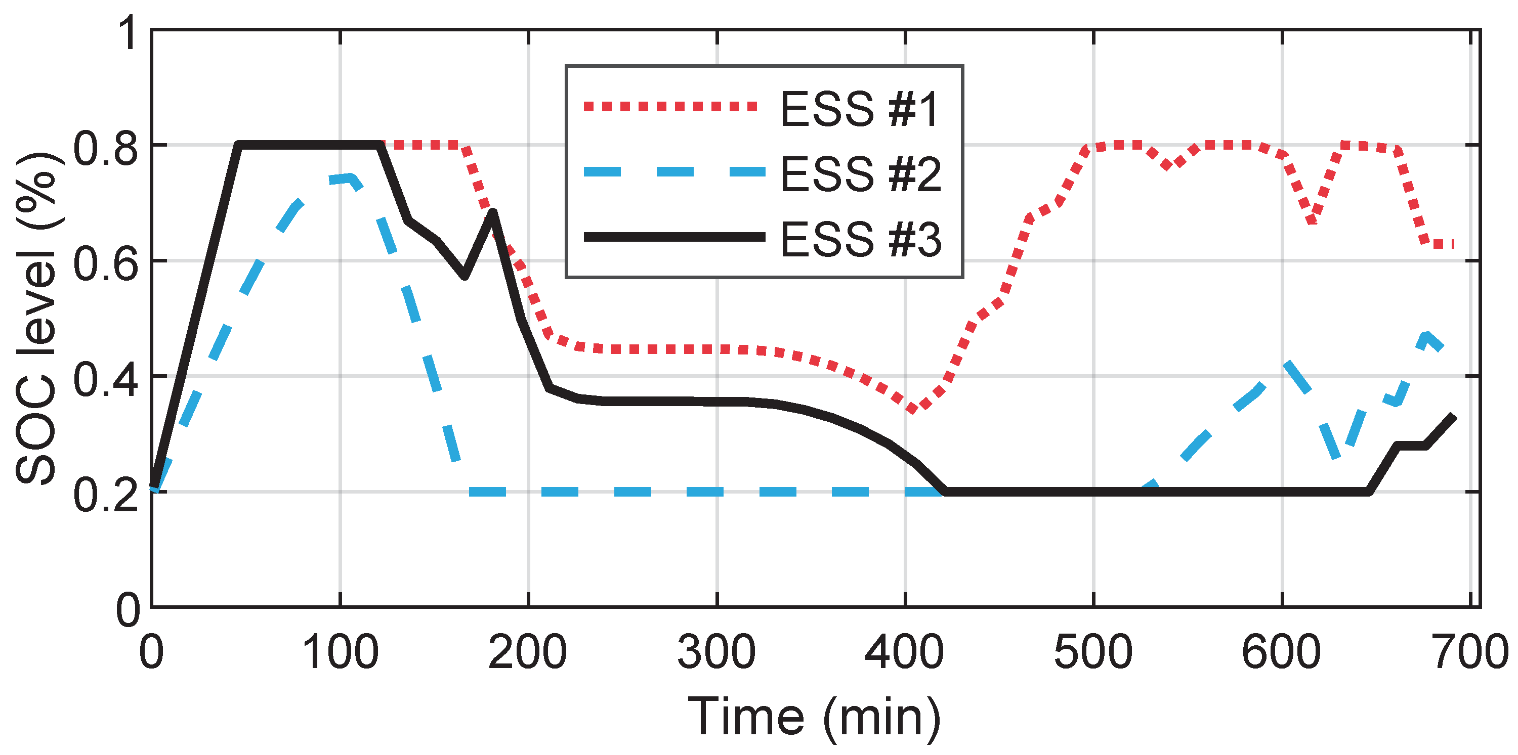
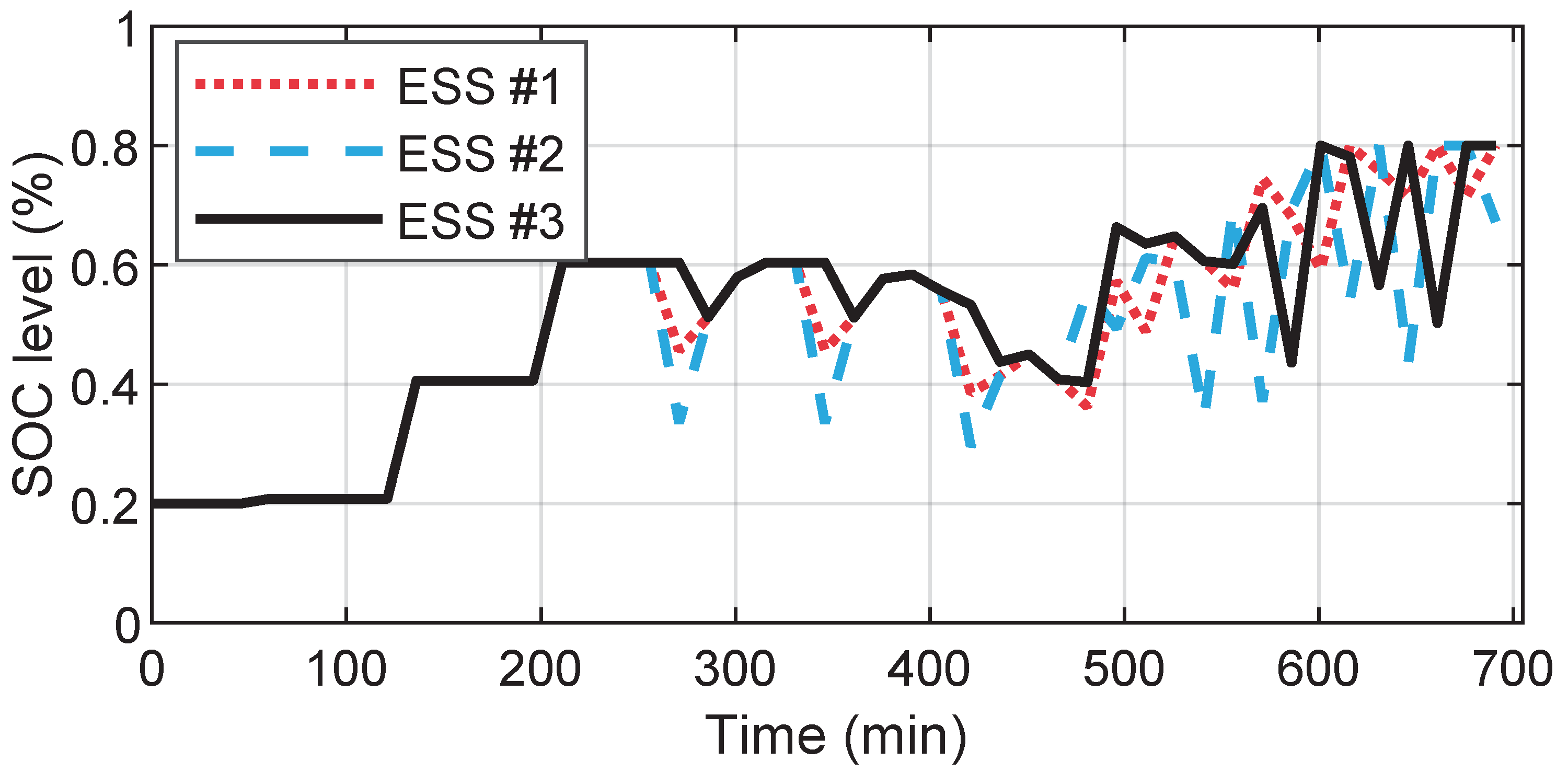
4.2.3. Role of Energy Storage in Recovery

Storage is necessary for the process of recovery. We notice that the control of ESS contains time-coupling constraints. From this perspective, the SOC changes of the two methods are further compared. The SOC changes of each storage are shown in Figure 8 and Figure 9.
Compared with the greedy method, the SOC curve obtained by the proposed method is more periodic. When the DER output is large, the excess energy is stored in the ESS. When the DER output is not enough to restore the power failure load, the ESS will provide an emergency power supply to the system. Since it introduces predictions in the optimization model, it can solve a better control strategy.

4.3. Analysis of Linearization

Our work involves two linearization techniques. Both of them are used for simplifying our model and accelerating the computational speed. In this section, we discuss the possible error that may be introduced.

4.3.1. Linearization of Power Flow Conversation Constraints

LinDistFlow is a used to linearize the power flow conversation constraints. It neglects the line losses. For a radial distribution network, the line losses are relatively small and have little effect on the results. In the tested 33-bus system, the ratio of line losses is less than 2%.
We further compare the results between LinDistFlow and AC power flow model for accuracy analysis. The mean value of absolute deviation (MAD) given in (35) is used to evaluate the differences between the two models.
MAD = 1 n i = 1 n v i t , A C v i t , L D F v i t , A C
where n is the number of restored loads at each bus; v i t , A C and v i t , L D F are the voltages calculated by the AC model and LinDistFlow model, separately.
We implement different models on the same case. The results show that the average voltage deviation MAD at each time t does not exceed 4%. Hence, it is acceptable to use LinDistFlow model in the restoration process.

4.3.2. Linearization of Line Capacity Constraints

The line capacity constraint is linearized to simplify the model and eliminate the strong nonlinearity. Usually, the line will not be overloaded through proper distribution network planning. That is, the line capacity constraint will not be violated. In the process of distribution network restoration, only part of the loads are picked up, so it is even less likely to violate the line capacity constraints. Therefore, the linearization technique is only used to improve the computational efficiency and speed up the model’s solution. It will not introduce errors to the results.

5. Conclusions

This paper investigates the coordination of network reconfiguration and DERs in the resilient restoration of damaged ADNs. When faced with extreme events, such as meteorological disasters, ADNs may be disconnected from the main grid and thus lose power supply. As a flexible form of energy, DERs can be used as an emergency power supply for the restoration of an ADN. Therefore, we establish a detailed multiperiod restoration model taking account of multiple DERs to deeply explore their potential on resilient restoration. The operation of ESS is also considered in the modeling process. It is used to smooth the fluctuations of loads and DER outputs. Then, we propose a rolling horizon optimization framework to solve this multiperiod model. The framework utilizes the predictions and avoids the influence of prediction errors on the optimal restoration strategy as much as possible.
The simulation results demonstrate the effectiveness of the proposed model. Compared with the traditional greedy method, the performance of network reconfiguration with multiple DERs has significantly improved. During the system restoration process, the load recovery rate at each moment has been significantly improved. At some moments, the load recovery rate increases by 20% compared with the traditional greedy method. In addition, due to the introduction of future forecast information, the strategy obtained by the rolling horizon optimization is closer to the optimal global solution, and all loads can be picked up within 420 min. However, the greedy strategy can only restore all loads at 660 min.

Author Contributions

Conceptualization, Y.S. and N.X.; methodology, N.X. and L.C.; software, N.X.; validation, N.X.; writing—original draft preparation, L.M. and Y.S.; writing—review and editing, L.C.; supervision, L.C.; project administration, L.M.; funding acquisition, L.M. All authors have read and agreed to the published version of the manuscript.

Funding

This work was funded by the Scientific and Technological Project of Qinghai Province (2021-ZJ-938Q).

Institutional Review Board Statement

Not applicable.

Informed Consent Statement

Not applicable.

Data Availability Statement

Not applicable.

Conflicts of Interest

The authors declare no conflict of interest.

References

  1. Lasseter, R.; Akhil, A.; Marnay, C.; Stephens, J.; Dagle, J.; Guttromsom, R.; Meliopoulous, A.S.; Yinger, R.; Eto, J. Integration of Distributed Energy Resources. The CERTS Microgrid Concept; Technical Report; Lawrence Berkeley National Lab. (LBNL): Berkeley, CA, USA, 2002. [Google Scholar]
  2. Peponis, G.; Papadopoulos, M.; Hatziargyriou, N. Distribution network reconfiguration to minimize resistive line losses. IEEE Trans. Power Deliv. 1995, 10, 1338–1342. [Google Scholar] [CrossRef]
  3. Dorostkar-Ghamsari, M.R.; Fotuhi-Firuzabad, M.; Lehtonen, M.; Safdarian, A. Value of distribution network reconfiguration in presence of renewable energy resources. IEEE Trans. Power Syst. 2015, 31, 1879–1888. [Google Scholar] [CrossRef]
  4. Zhu, D.; Cheng, D.; Broadwater, R.P.; Scirbona, C. Storm modeling for prediction of power distribution system outages. Electr. Power Syst. Res. 2007, 77, 973–979. [Google Scholar] [CrossRef]
  5. Rao, R.S.; Ravindra, K.; Satish, K.; Narasimham, S. Power loss minimization in distribution system using network reconfiguration in the presence of distributed generation. IEEE Trans. Power Syst. 2012, 28, 317–325. [Google Scholar] [CrossRef]
  6. Han, S.R. Estimating Hurricane Outage and Damage Risk in Power Distribution Systems; Texas A&M University: College Station, TX, USA, 2008. [Google Scholar]
  7. Chen, C.; Wang, J.; Qiu, F.; Zhao, D. Resilient distribution system by microgrids formation after natural disasters. IEEE Trans. Smart Grid 2016, 7, 958–966. [Google Scholar] [CrossRef]
  8. Ding, T.; Lin, Y.; Bie, Z.; Chen, C. A resilient microgrid formation strategy for load restoration considering master-slave distributed generators and topology reconfiguration. Appl. Energy 2017, 199, 205–216. [Google Scholar] [CrossRef]
  9. Lee, C.; Liu, C.; Mehrotra, S.; Bie, Z. Robust distribution network reconfiguration. IEEE Trans. Smart Grid 2014, 6, 836–842. [Google Scholar] [CrossRef]
  10. Ma, S.; Chen, B.; Wang, Z. Resilience enhancement strategy for distribution systems under extreme weather events. IEEE Trans. Smart Grid 2018, 9, 1442–1451. [Google Scholar] [CrossRef]
  11. Lei, S.; Hou, Y.; Qiu, F.; Yan, J. Identification of critical switches for integrating renewable distributed generation by dynamic network reconfiguration. IEEE Trans. Sustain. Energy 2017, 9, 420–432. [Google Scholar] [CrossRef]
  12. Wu, T.; Wang, J.; Lu, X.; Du, Y. AC/DC hybrid distribution network reconfiguration with microgrid formation using multi-agent soft actor-critic. Appl. Energy 2022, 307, 118189. [Google Scholar] [CrossRef]
  13. Li, B.; Chen, Y.; Wei, W.; Huang, S.; Mei, S. Resilient Restoration of Distribution Systems in Coordination with Electric Bus Scheduling. IEEE Trans. Smart Grid 2021, 12, 3314–3325. [Google Scholar] [CrossRef]
  14. Nikkhah, S.; Jalilpoor, K.; Kianmehr, E.; Gharehpetian, G.B. Optimal wind turbine allocation and network reconfiguration for enhancing resiliency of system after major faults caused by natural disaster considering uncertainty. IET Renew. Power Gener. 2018, 12, 1413–1423. [Google Scholar] [CrossRef]
  15. Hamid-Oudjana, S.; Mosbah, M.; Zine, R.; Arif, S. Optimum Dynamic Network Reconfiguration in Smart Grid Considering Photovoltaic Source. In Proceedings of the International Conference in Artificial Intelligence in Renewable Energetic Systems, Taghit, Bechar, Algeria, 24–26 November 2019; pp. 557–565. [Google Scholar]
  16. Jiang, L.; Chen, W.; Chen, Y.; Lai, J.; Yin, X. Resilient Control Strategy Based on Power Router for Distribution Network with Renewable Generation. In Proceedings of the 10th Renewable Power Generation Conference (RPG 2021), Online, 14–15 October 2021. [Google Scholar]
  17. Lei, S.; Chen, C.; Li, Y.; Hou, Y. Resilient Disaster Recovery Logistics of Distribution Systems: Co-Optimize Service Restoration with Repair Crew and Mobile Power Source Dispatch. IEEE Trans. Smart Grid 2019, 10, 6187–6202. [Google Scholar] [CrossRef] [Green Version]
  18. Yang, Z.; Dehghanian, P.; Nazemi, M. Enhancing seismic resilience of electric power distribution systems with mobile power sources. In Proceedings of the 2019 IEEE Industry Applications Society Annual Meeting, Baltimore, MD, USA, 29 September–3 October 2019; pp. 1–7. [Google Scholar]
  19. Kianmehr, E.; Nikkhah, S.; Vahidinasab, V.; Giaouris, D.; Taylor, P.C. A resilience-based architecture for joint distributed energy resources allocation and hourly network reconfiguration. IEEE Trans. Ind. Inform. 2019, 15, 5444–5455. [Google Scholar] [CrossRef]
  20. Li, B.; Chen, Y.; Wei, W.; Mei, S.; Hou, Y.; Shi, S. Preallocation of Electric Buses for Resilient Restoration of Distribution Network: A Data-Driven Robust Stochastic Optimization Method. IEEE Syst. J. 2021, 1–12. [Google Scholar] [CrossRef]
  21. Li, B.; Chen, Y.; Wei, W.; Huang, S.; Xiong, Y.; Mei, S.; Hou, Y. Routing and Scheduling of Electric Buses for Resilient Restoration of Distribution System. IEEE Trans. Transp. Electrif. 2021, 7, 2414–2428. [Google Scholar] [CrossRef]
  22. Elsayed, W.T.; Farag, H.; Zeineldin, H.H.; El-Saadany, E.F. Formation of Islanded Droop-Based Microgrids with Optimum Loadability. IEEE Trans. Power Syst. 2021, 37, 1564–1576. [Google Scholar] [CrossRef]
  23. Low, S.H. Convex relaxation of optimal power flow—Part I: Formulations and equivalence. IEEE Trans. Control. Netw. Syst. 2014, 1, 15–27. [Google Scholar] [CrossRef] [Green Version]
  24. Sethi, S.; Sorger, G. A theory of rolling horizon decision making. Ann. Oper. Res. 1991, 29, 387–415. [Google Scholar] [CrossRef]
  25. Li, B.; Chen, Y.; Wei, W.; Wang, Z.; Mei, S. Online Coordination of LNG Tube Trailer Dispatch and Resilience Restoration of Integrated Power-Gas Distribution Systems. IEEE Trans. Smart Grid 2022, 13, 1938–1951. [Google Scholar] [CrossRef]
Figure 1. An illustration of the network reconfiguration.
Energies 15 03096 g001
Figure 2. An illustration for linearization.
Energies 15 03096 g002
Figure 3. Schematic representation of the rolling horizon optimization from time t to time t + 1 .
Energies 15 03096 g003
Figure 4. The situation of damaged lines for the test system.
Energies 15 03096 g004
Figure 5. Load curve between 6:00 a.m. and 6:00 p.m.
Energies 15 03096 g005
Figure 6. DER outputs curve between 6:00 a.m. and 6:00 p.m.
Energies 15 03096 g006
Figure 7. The comparison of load restoration between the greedy method and the proposed framework.
Energies 15 03096 g007
Figure 8. The change of each ESS’s SOC using greedy method.
Energies 15 03096 g008
Figure 9. The change of each ESS’s SOC using proposed rolling horizon method.
Energies 15 03096 g009
Table 1. Restored time of damage equipment [25].
Distribution Line
Index23–2419–209–156–76–269–1012–1329–30
min240300360420480540600660
Publisher’s Note: MDPI stays neutral with regard to jurisdictional claims in published maps and institutional affiliations.

