Article

Large-Eddy Simulation of Wakes of Waked Wind Turbines

1
The State Key Laboratory of Nonlinear Mechanics, Institute of Mechanics, Chinese Academy of Sciences, Beijing 100190, China
2
School of Engineering Sciences, University of Chinese Academy of Sciences, Beijing 100049, China
3
Civil and Environmental Engineering Department, Hanyang University, Seoul 133791, Korea
4
Civil Engineering Department, Stony Brook University, Stony Brook, NY 11794, USA
*
Author to whom correspondence should be addressed.
Energies 2022, 15(8), 2899; https://doi.org/10.3390/en15082899
Submission received: 16 March 2022 / Revised: 12 April 2022 / Accepted: 13 April 2022 / Published: 15 April 2022
(This article belongs to the Section A3: Wind, Wave and Tidal Energy)

Abstract

:
The wake dynamics of a wind turbine are influenced by the atmospheric turbulence and the wake of its upwind turbine. In this work, we investigate the wake characteristics of a waked wind turbine for four different downwind spacings and three different inflows using large-eddy simulation with a turbine parameterized using the actuator surface model. The wake statistics of the waked turbine are compared with those of the stand-alone wind turbine under the same inflow. The results show that the oncoming wake significantly affects the near wake of the waked turbine, where it accelerates the wake recovery by increasing the turbulent convection, and increases the turbulence kinetic energy. The velocity deficit and turbulence kinetic energy in the far wake, on the other hand, are fairly similar with each other for the considered different turbine spacings, and are close to those of the stand-alone wind turbine. As for the wake meandering of the waked wind turbines, it is initiated quickly and enhanced by the oncoming wake turbulence, as shown by the meandering amplitudes and the power spectral density of the instantaneous wake positions. The growth rates of the wake meandering from the waked wind turbines, on the other hand, are close to that of the stand-alone wind turbine, indicating the critical role of the atmospheric turbulence on wake meandering. The present work details how the oncoming wake influences the wake dynamics of the downwind turbine, and provides physical insights on developing engineering models to take into account such effects.

1. Introduction

Wind turbine wake is one of the key factors affecting wind farm performance [1]. Its effects on downwind turbines are influenced by turbine spacings, ambient turbulence and several other factors [2]. A two tandem turbine array is the simplest case for studying the influence of an upwind turbine’s wake on the downwind one. This work is devoted to studying how the wake from an upwind wind turbine affects the wake dynamics of a downwind turbine in a two tandem turbine array setup for different turbine spacings and under different turbulent inflows.
The wake of a wind turbine is often divided into the near wake region and the far wake region [3]. In the near wake, the flow structure is featured by tip vortices and a hub vortex, in which the former ones decay quickly under turbulent inflows. Chen et al. [4]. investigated the effects of turbulence on the instability of tip vortices. The characteristics of the vortex structures in the near wake of the Eolos turbine at University of Minnesota were investigated by Dasari et al. [5]. Downwind evolution of tip vortices was also investigated by Na et al. [6]. In the work of Yang et al. [7], tip vortices with tails and secondary vortices in the near wake of the Eolos turbine were discovered in large-eddy simulations and field observations using snow particles as tracers [8]. The far wake, on the other hand, is featured by a low-frequency, large-scale meandering motion, which has pronounced effects on the power extraction and dynamic loads of downwind turbines. Two different mechanisms have been identified for the onset of wake meandering, i.e., (1) the inflow large eddy mechanism [9,10], and (2) the shear layer instability mechanism [11,12]. Wake meandering has been observed in both lab-scale and field-scale wind turbines (e.g., [13,14]) and for different operating regimes [15]. Using field measurements, Brugger et al. [16] found that the correlation between the instantaneous wake position and the lateral velocity decreases as one travels downstream. Field observations and numerical simulations suggested the co-existence of the two mechanisms [10,17]. Hub vortex plays an important role in the onset of wake meandering caused by the shear layer instability [12,18,19,20]. The importance of accurately taking into account the nacelle effect was shown in the literature for both stand-alone turbines and utility-scale wind farms [12,21]. A recent review on wake meandering can be found in the paper by Yang and Sotiropoulos [22].
Wake dynamics are affected by factors such as the ambient turbulence and oncoming turbine wakes. Uchida [23] investigated how the wind shear affects the time-averaged velocity and turbulence statistics in turbine wakes. Decillis et al. [24] analyzed the effects of different flow structures on wake recovery. Studies showed that inflow turbulence can accelerate the wake recovery [25,26]. The effects of atmospheric stability on turbine wakes were investigated numerically and experimentally [27,28]. Churchfield et al. [29] investigated the effects of atmospheric and wake turbulence on the power production and loads of downwind turbines for different stratification and surface roughness conditions. Herges et al. [30] analyzed the field data at the SWiFT facility to probe into how an upstream wake influences turbine power and blade loads of the downwind turbine. They found that the fatigue load is higher for partial wake impingement when compared with the full wake. Investigations on the topology effect on turbine wakes were carried out in the literature using simulations, wind tunnel experiments and field measurements [31,32,33]. Wang et al. [34] simulated the flow past two and three aligned turbines (of rotor diameter 1.1 m) with streamwise spacing of 4.1 rotor diameters and compared the simulation results with the measurements. Using a wind tunnel experiment, Bartl et al. [35] found that the velocity profile of the waked turbine is similar to that of a stand-alone turbine. Adaramola and Krogstad [36] investigated the effects of turbine spacing on power output using a wind tunnel experiment. In the work of Mycek et al. [37], the flow past two turbines under different inflow turbulence intensities was investigated in a wind tunnel for different turbine spacings.
Similarity in wind turbine wakes plays a critical role in developing engineering models, which are often employed in the design and control optimization of wind farms [38]. In the work by Xie et al. [39], self-similarity was studied for different wind speeds, operating conditions and with/without a nacelle. Self-similarity of the velocity deficit in the wake of a yawed wind turbine was shown by Bastankhah and Porté-Agel [40]. Self-similar characteristics of wake-added turbulence intensity were investigated by Li et al. [41]. Similarity between wakes of different turbine designs was shown in large-eddy simulations by Foti et al. [42]. In a recent work, Li and Yang [43] showed that the wakes from turbines with different yaw angles are similar with each other when the quantities of interest are scaled with the proposed length and velocity scales, indicating that one can estimate the wake characteristics for different yaw angles based on the results at one yaw angle.
Different engineering models for turbine wakes have been developed in the literature, including the effective roughness models, kinematic models and hybrid models [44,45,46,47,48]. Efforts on developing a reduced-order wake model using proper orthogonal decomposition can be found in the work by Moon et al. [49]. Recent development on engineering models taking into account wake meandering effects can be found in Shaler et al.’s work [50]. In the work by Yang [51], a neural network model for predicting the instantaneous wake positions was developed. See Appendix A. To account for upstream wakes, different wake superposition methods have been proposed in the literature [2,52]. In Zong et al.’s work [53], a wake superposition method conserving the total momentum deficit was developed. A wake merging method considering a heterogeneous background velocity field was developed by Lanzilao and Meyers [54]. Studies on turbine arrays of different spacings and layouts have been reported [45,48,55], focusing on the power output and the cumulative effect of turbines and turbine wakes as the effective roughness. To mitigate the effects of turbine wakes, different control strategies were developed in the literature [56,57,58]. The active control of the power production of wind farms was investigated to consider wind turbine wake effects [59,60,61].
Although many research efforts on wind turbine wakes exist in the literature, as discussed above, there is still a lack of knowledge on how the oncoming wake turbulence affects the wake of a downwind turbine. In the literature, the effect of inflow turbulence was often investigated without differentiating the different effects of the atmospheric turbulence and oncoming wake turbulence [25,32]. The integral scale of the turbulence induced by turbine wakes is, in general, significantly smaller than that of the atmospheric turbulence. Compared with the atmospheric turbulence, it is not clear how different the oncoming wake turbulence affects the wake characteristics of waked wind turbines. For instance, will the oncoming wake turbulence increase the wake recovery in the same way as the atmospheric turbulence? How does the oncoming wake turbulence affect the wake turbulence of the waked turbine? And will the oncoming wake turbulence enhance the wake meandering of the waked wind turbine? To address these questions, in this work, we carry out large-eddy simulations of flows past two aligned wind turbines with different turbine spacings under different turbulent inflows. Specifically, we examine the influences of the oncoming wake on both time-averaged wake and wake meandering of the waked turbine, and compare them with those of a stand-alone wind turbine.
The rest of the paper is organized as follows. The employed numerical methods and the simulation setup are introduced in Section 2. Then, the simulation results are presented in Section 3. At last, the conclusions are drawn in Section 5.

2. Numerical Methods and Simulation Set-Up

2.1. Numerical Methods

The large-eddy simulation (LES) module of the Virtual Flow Simulator (VFS-Wind) code [62,63], which has been successfully employed to simulate flows in different applications, e.g., wind energy [64], hydrokinetic energy [65], pollutant transport [66], blood flows [67], flows over underwater vehicles [68,69] and rough wall turbulence [64], was employed in this work. Validation of the VFS-Wind code with the laboratory-scale and field-scale measurements for predicting wind turbine wakes can be found in our previous work [7,62,70,71]. The governing equations are the filtered incompressible Navier–Stokes equations as follows:
u j x j = 0 ,
u i t + u i u j x j = 1 ρ p x i + x j ν + ν t u i x j + f i ,
where i , j = 1 , 2 , 3 , u is the velocity, p is the pressure, ν is the kinematic viscosity, ν t is the eddy viscosity modeled using the Smagorinsky model with the model coefficient determined following the dynamic procedure [72] and f i is the body force (per unit mass) from the actuator surface model to represent the effects of both turbine blades and nacelle.
The actuator surface model developed by Yang and Sotiropoulos [70] was employed in this work, which avoids the need to resolve the boundary layer over the blade and thus is more computationally efficient than geometry-resolved simulations [12], and is more accurate than actuator disk/actuator line model [48,62] by better taking into account the geometrical effect in the chordwise direction. In the actuator surface model for blades, the blade is represented by a surface formed by chords at different radial locations. Surface forces, which are uniformly distributed in the chordwise direction, model the interaction between the blades and the incoming flow. The chordwise-integrated force at each radial location is determined via the blade element method using the local relative incoming velocity and the tabulated geometric and aerodynamic information. In the turbine parameterization methods, the grids for representing the actuator surface and solving the flow field are independent of each other. The information between the two sets of grids is transferred using the smoothed discrete delta function of Yang et al. [73].
The governing equations are spatially discretized using a second-order central difference scheme, and advanced in time using the second-order fractional step method [74]. The discretized momentum equation is solved using a matrix-free Newton–Krylov method [75]. The Poisson equation for satisfying the divergence-free constraint is solved using the Generalized Minimal Residual (GMRES) method with an algebraic multi-grid acceleration [76].

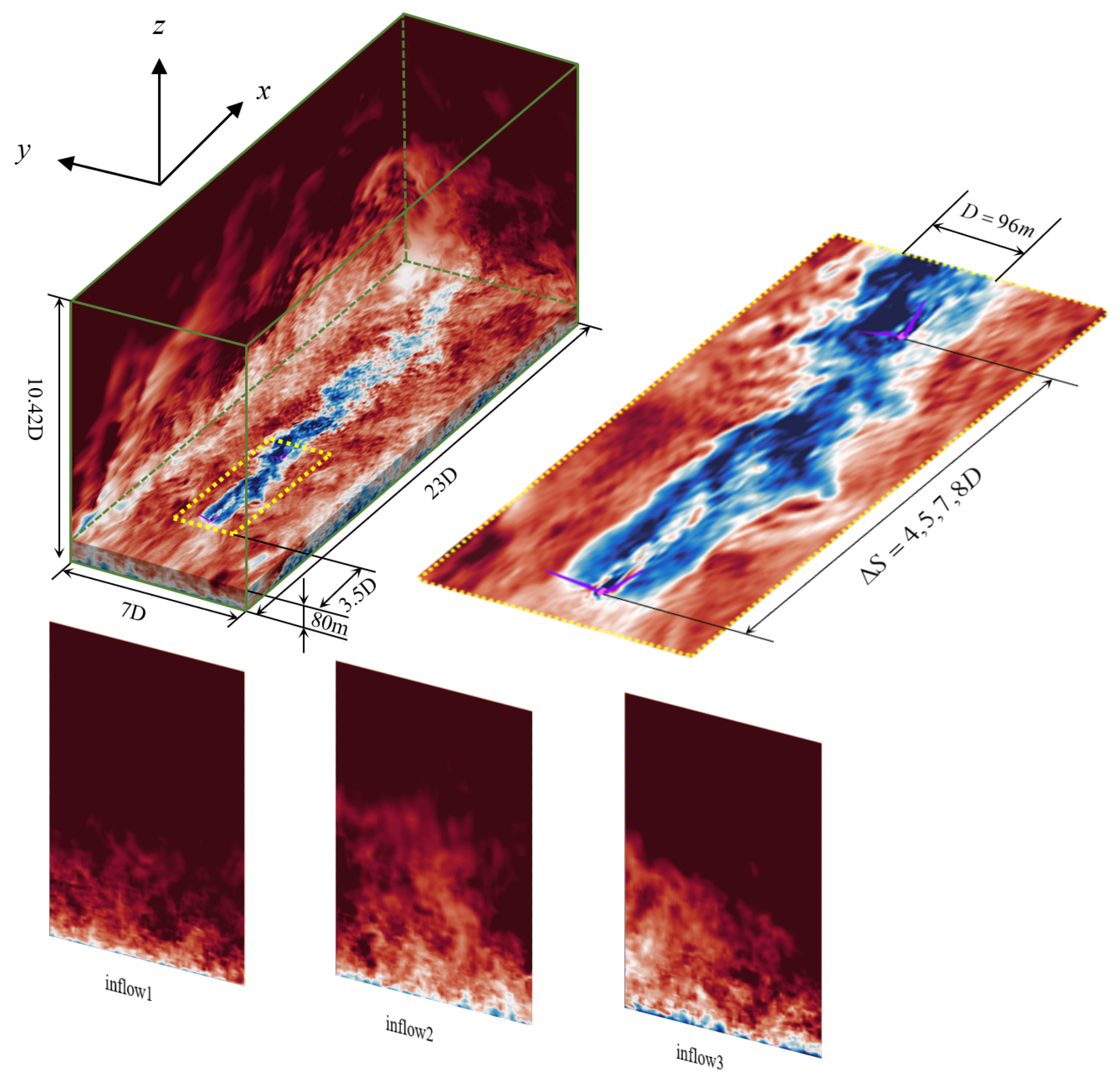
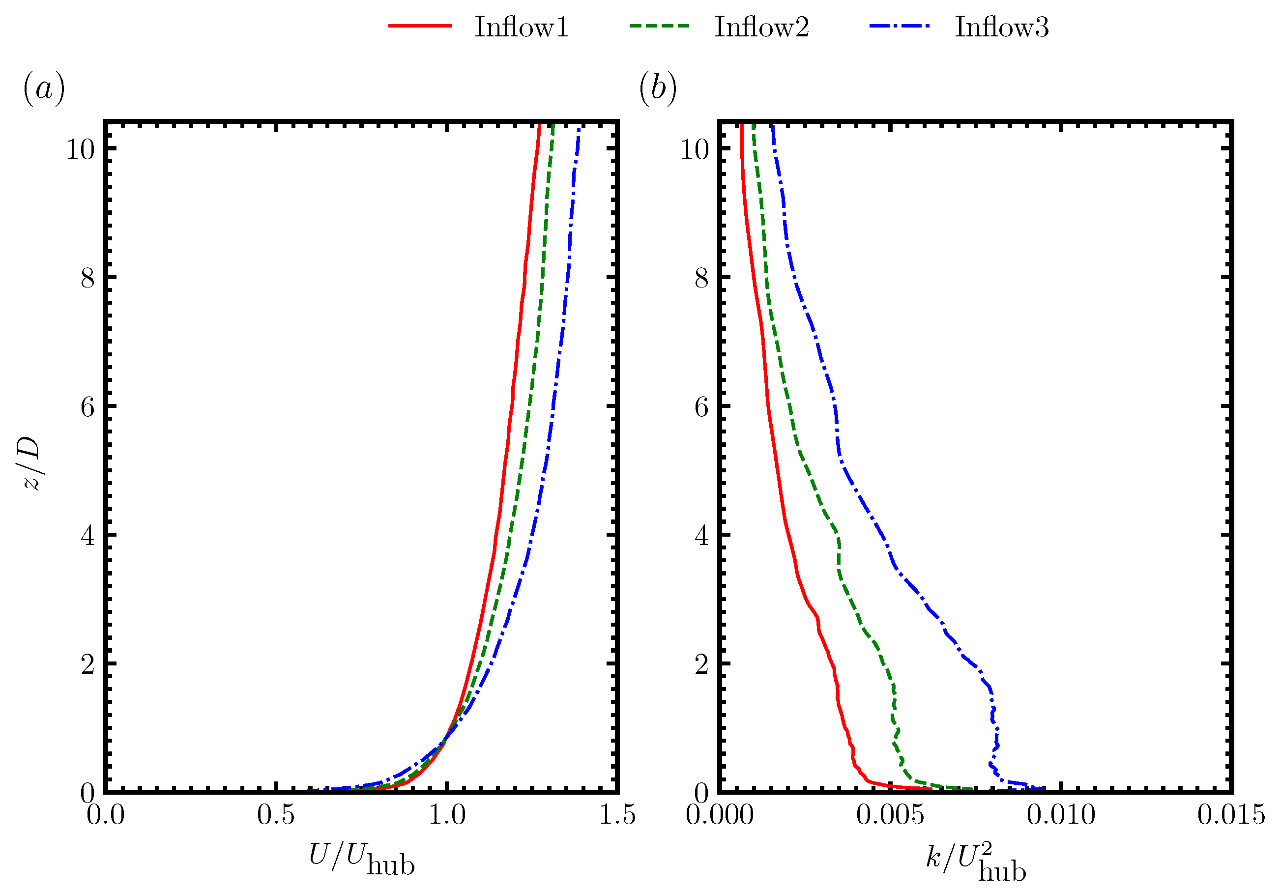
2.2. Simulation Set-Ups

In this section, we present the set-ups of the simulated cases. The 2.5 MW Eolos wind turbine with rotor diameter D = 96 m and hub height z h = 80 m, at the University of Minnesota, was employed in the present work. Because of proprietary reasons, the blade data, such as the airfoil type, lift and drag coefficients, which are important parameters for a wind turbine [77], cannot be provided in this paper. The readers can contact the Eolos Wind Research station at the University of Minnesota for these data. Other details on the Eolos wind turbine can be found in [8].
Downwind turbine spacings of 7 D or 8 D are typical for utility-scale wind farms [78], although larger turbine spacings exist in different wind farms [79], as suggested in the literature [80]. For other circumstances, the turbines may also be close to each other, especially for wind blowing from a direction different from the predominant direction. Considering the dominant effects of wakes on downwind turbines for short turbine spacings, two typical downwind turbine spacings ( Δ S = 7 , 8 D ) together with two short spacings ( Δ S = 4 , 5 D ), as shown in Figure 1, were considered in this work. The length, width and height of the computational domain were 23 D , 7 D and 10.42 D in the streamwise (x), spanwise (y) and vertical (z) directions, respectively, with the corresponding numbers of grid nodes N x × N y × N z = 461 × 281 × 143 . The grid nodes were uniformly distributed in the x, y directions with the grid spacing Δ x = D / 20 and Δ y = D / 40 , respectively. In the z direction, the grid was uniform for z / D < 2 with Δ z = D / 40 and gradually stretched to the top boundary. The resolution of the employed grid was typical for actuator type simulations [2,22,52]. A grid refinement study has been carried out in our previous work [43], showing that the employed grid is enough to predict the quantities of interest in this work. In addition to the two-turbine cases, stand-alone turbine cases were also carried out for different surface roughness lengths, in which the turbine was located at the same location as the first turbine in the two-turbine cases. In the analysis carried out in this work, x c , y c and z c were employed to denote the position of the turbine to facilitate the comparison in the coordinate with its origin located at the corresponding turbine. For comparison with reference to the inlet position, x c 0 was employed to denote the streamwise coordinate of the stand-alone turbine and that of the first turbine for the two-turbine cases.
The free-slip boundary condition was applied at boundaries in the spanwise direction and at the top boundary. At the bottom boundary, the logarithmic law for rough wall was employed as the wall model to compute wall shear stress, together with the non-penetration condition for the wall-normal velocity, serving as the approximate boundary conditions for the outer flow simulations. At the outlet, the Neumann boundary condition was employed. At the inlet, turbulent inflows with three different roughness lengths, i.e., k 0 = 0.001 m, 0.01 m and 0.1 m dubbed as inflow1, inflow2 and inflow3, respectively, were applied, which were obtained from precursory simulations, in which a large computational domain (i.e., L x × L y × L z = 2250 m × 1487 m × 1000 m with the number of grid nodes N x × N y × N z = 1126 × 1488 × 152 ) was employed to capture the large-scale eddies in atmospheric turbulence. In the precursory simulations, periodic boundary conditions were applied in the horizontal directions. At the top boundary and the wall, the same boundary conditions as those in the turbine cases were applied. In the precursory simulations, the velocity fields on a y z plane were saved at each time step. The inflow boundary condition for the wind turbine simulations were then obtained with linear interpolations in both time and space from the saved velocity fields. A summary of the cases carried out in this work is shown in Table 1.
The mean streamwise velocity profiles and turbulence kinetic energy profiles from inflow1, inflow2 and inflow3 are shown in Figure 2. As seen, with the increase of surface roughness, the normalized streamwise velocity decreases in the near wall region, with the increase of turbulence kinetic energy at all the vertical locations.
The power and thrust of the waked turbine, which were normalized using that of the first turbine, are shown in Figure 3. As expected, the normalized power ( P 2 / P 1 ) and thrust ( T 2 / T 1 ) increased with downwind turbine spacing and the increase of the inflow turbulence intensity, as the former one increased the downwind distance for wake recovery and the latter one increased the rate of wake recovery.

3. Results

In this section, we analyze the results from cases with different downwind turbine spacings and different inflows. We compare the wake of the waked turbine with that of the stand-alone turbine.

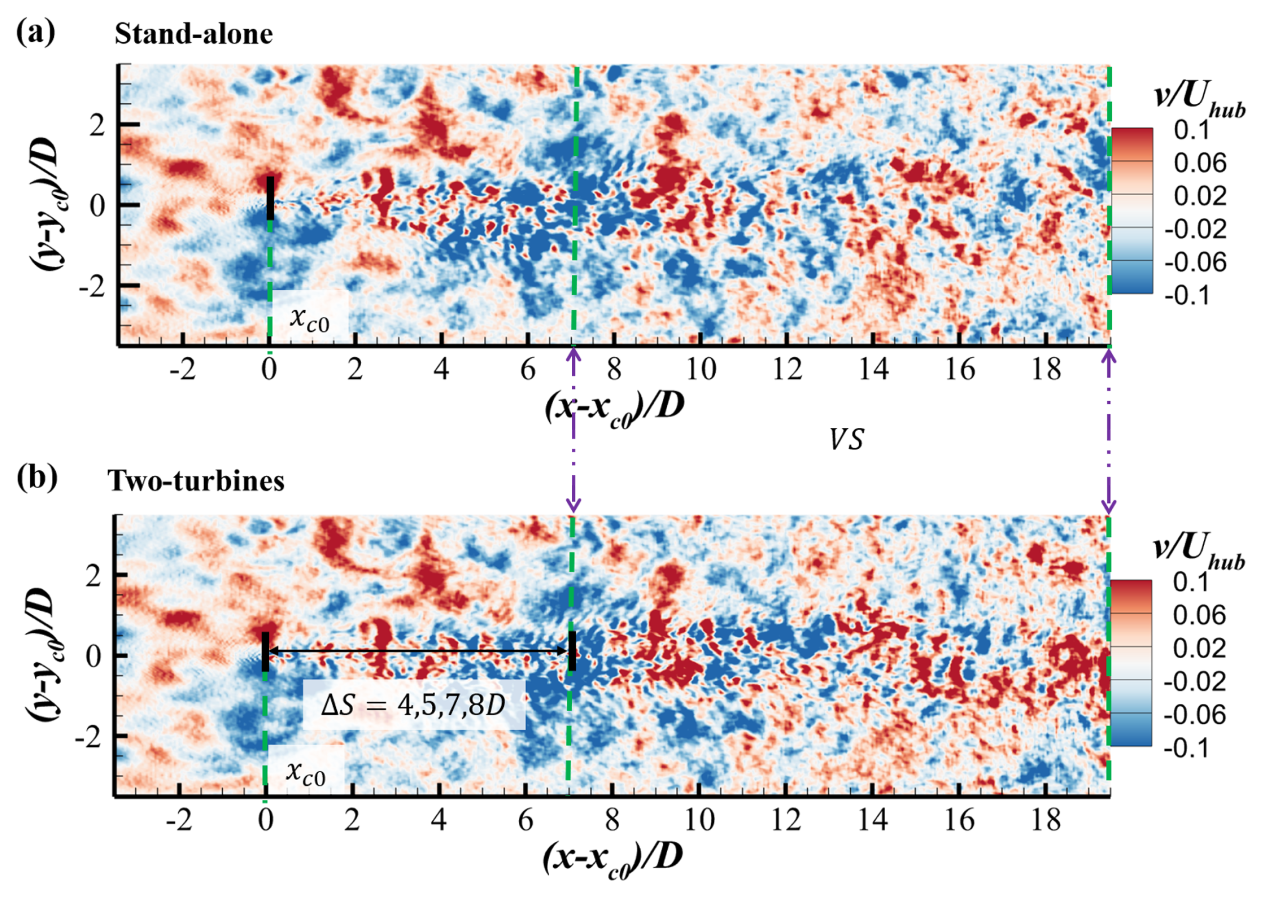
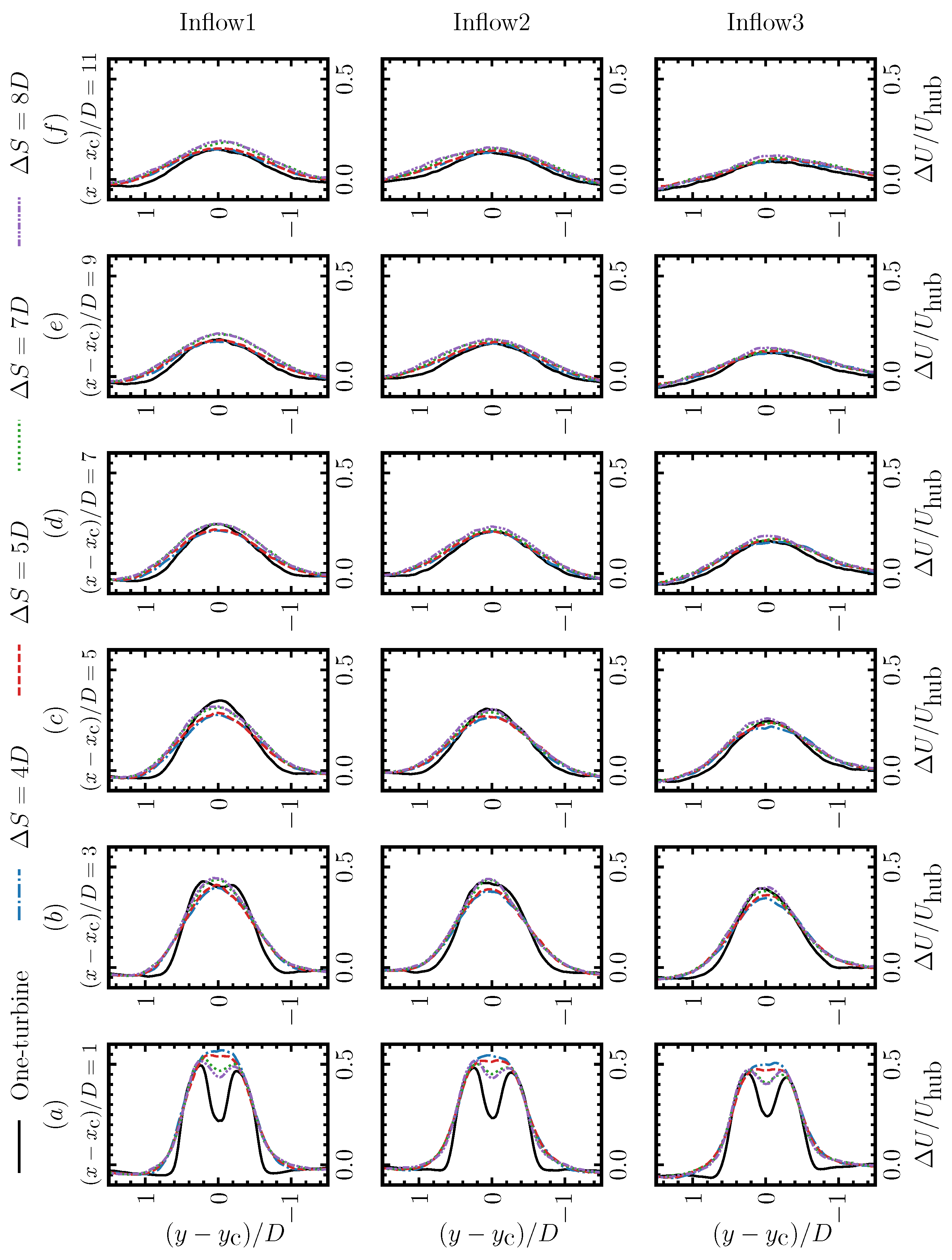
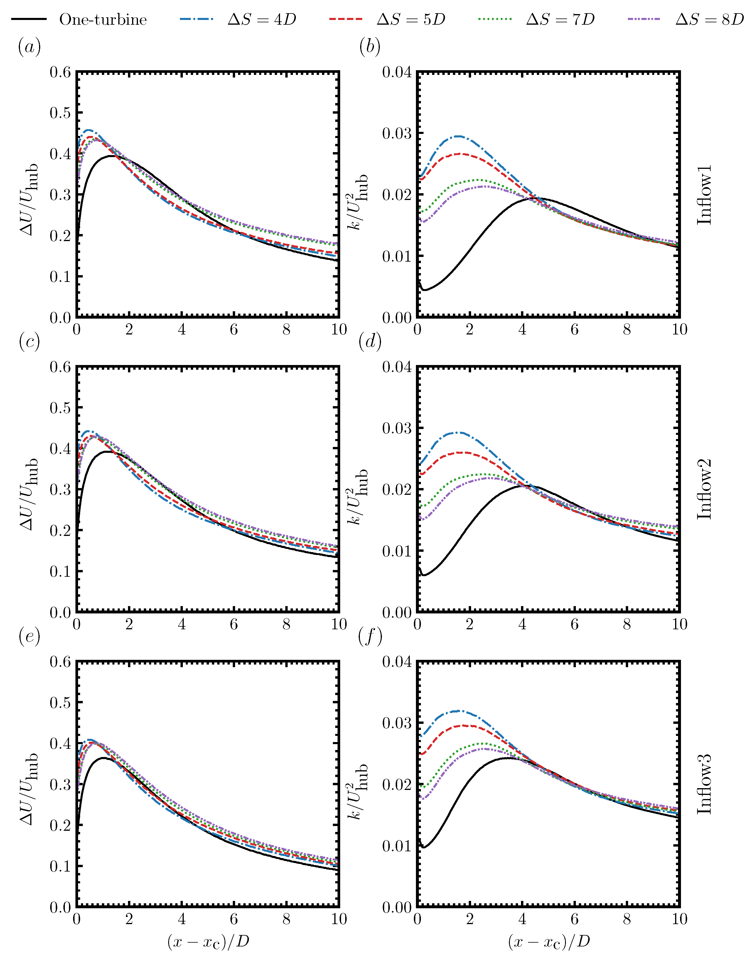
3.1. Instantaneous and Time-Averaged Wake Characteristics

We examined the instantaneous flow field and the statistics of the time-averaged wake in this section. Two comparison schemes based on different coordinate systems were employed, which are illustrated in Figure 4 and Figure 5, before the detailed analyses in this and the following sections.
First, we show the instantaneous streamwise and spanwise velocity in Figure 4 and Figure 5, respectively, for both the stand-alone and two-turbine cases at the same time instant. Two typical features of wind turbine wakes are observed in Figure 4, i.e., the velocity deficit and the wake meandering. Significant meandering of the first turbine (or the stand-alone wind turbine) started at about 2 D turbine downstream, which started almost immediately for the second wind turbine. If examined carefully, certain similarities are observed between the spanwise position of the near wake of the second turbine and that of the stand-alone wind turbine at the same streamwise locations.
When considering wake meandering as the result of inflow large eddies, spanwise velocity is the main cause for the spanwise displacement of wind turbine wakes. It is seen in Figure 5 that the large-scale pattern of the spanwise velocity in the near wake of the second turbine was close to that of the stand-lone turbine at the same streamwise location, indicating that their wake meandering may share some similarities although the distances from the corresponding wind turbine were different. The observations from the cases with different surface roughness lengths and turbine spacings were similar, which will not be further examined.
Two comparison schemes are shown in Figure 4 and Figure 5. In this paper, most analyses (e.g., Figure 6, Figure 7, Figure 8, Figure 9, Figure 10, Figure 11, Figure 12 and Figure 13) were carried out based on the scheme shown in Figure 4 with reference to the corresponding turbine location (the comparison scheme shown in Figure 4), except for Figure 14 where the comparison scheme shown in Figure 5 was employed.
In Figure 6, we compare the spanwise profiles of the streamwise velocity deficits ( Δ U = U hub U ) downwind of the second turbine of the two-turbine cases with those downwind of the stand-alone turbine. In the near wake, the velocity deficit profiles of the second turbine from the two-turbine cases with Δ S = 4 D , 5 D were close to the Gaussian distribution at the 1 D turbine downwind. In contrast, the velocity deficit profiles for the stand-alone turbine case and the two-turbine cases with Δ S = 7 D , 8 D were close to the double-Gaussian distribution with a low velocity deficit region near the hub. At further turbine downwind locations, the differences between the wake of the waked turbine and the stand-alone turbine became less significant. The major difference observed was that the wake of the waked turbine was broader than the stand-alone turbine. Effects of inflow conditions on the distribution of the streamwise velocity deficit were observed; the velocity deficit was smaller and was distributed in a wider wake region as a result of the enhanced mixing due to the increased ambient turbulence.
Figure 7 shows the spanwise profiles of the Reynolds stress u v downwind of the second turbine of the two-turbine cases and compares them with those downwind of the stand-alone turbine. Similar to the comparison of the streamwise velocity deficit profiles, the major differences between the wakes of the waked turbine and the stand-alone turbine were observed at the 1 D , 3 D turbine downwind locations. At the 1 D turbine downwind location, the overall variations of the Reynolds stress u v from the waked turbine were similar to that from the stand-alone turbine. However, the magnitudes of the u v from the waked turbine were larger than those from the stand-alone turbine at locations near ( y y c ) / D = ± 0.5 . The region with large magnitudes of u v was also wider for the waked turbine when compared with the stand-alone turbine. At the 3 D turbine downwind locations, the differences were still observed in terms of the magnitudes and the width of the region with high-magnitude u v . At further turbine downwind locations, the differences in the magnitudes of u v between the waked turbine and the stand-alone turbine became less distinct. The region with high-magnitude u v , on the other hand, was still somewhat wider at these downwind locations for the waked wind turbines. The wider region with high-magnitude u v indicates that the turbulence-induced momentum mixing between the wake and the ambient flow happens in a wider region for the waked turbine. This enhanced momentum mixing in the near wake was strongly correlated with wake meandering, which immediately happens in the downwind of the waked wind turbine, as will be shown later in this paper. It is important to notice that the spanwise profiles of u v from the waked wind turbine with different turbine spacings were very similar with each other, especially at 3 D and further turbine downwind locations for all the considered inflows.
Figure 8 shows the spanwise profiles of the turbulence kinetic energy k downwind of the second turbine of the two-turbine case and compares them with those downwind of the stand-alone turbine. Similar with those observed in the comparisons of the streamwise velocity deficit and Reynolds shear stress, the major differences in turbulence kinetic energy between the waked turbine and stand-alone turbine were observed at near wake locations (i.e., 1 D and 3 D turbine downwind). It was seen that at the 1 D turbine downwind the magnitude of the peak of the turbulence kinetic energy of the waked turbine was approximately twice of that of the stand-alone turbine. At the 3 D turbine downwind, the magnitude of the maximum k was still 15% to 25% higher than that of the stand-alone turbine. At further turbine downwind locations, although the high-magnitude turbulence kinetic energy was still distributed in a wider region for the waked turbine, the magnitude of the maximum k from the waked turbine was similar to that of the stand-alone turbine. Furthermore, the expansion of the shear layer near the edge of the wake could be clearly identified based on the distribution of k, that the two peaks were gradually flattened with the increase of downwind distance, indicating the converge of the shear layer at the center of the wake. Moreover, the hub vortex, which can be indicated by the two peaks in the hub region at 1 D turbine downwind, was inconspicuous in the wake of the waked wind turbine. Similar with u v , changing turbine spacings did not affect the spanwise distributions of k at 5 D and further downwind locations for the waked wind turbine. It was noticed that both u v and k were plotted without decomposing them to separate the contributions from the inflow turbulence (including atmospheric turbulence and oncoming wake turbulence) and turbine-added turbulence, and both were normalized using U h u b , the free stream incoming wind speed at hub height. Further analysis on the scaling of turbine-added turbulence for waked wind turbines, for which U h u b might not be the proper velocity scale, will be carried out in the future work.
To better show how turbulence kinetic energy k and velocity deficit Δ U vary in the streamwise direction, we show the disk-averaged k and Δ U via x in Figure 9. The circular disk employed for averaging has its center located along the axis of the rotor and its radius the same as the rotor radius R. We first examined the streamwise variations of the velocity deficit. It was seen that the overall variations of Δ U were similar for different cases, that Δ U first increased in the near wake and then gradually decreased as one travels to further turbine downwind locations. For the stand-alone turbine case, the maximum velocity deficit, with its locations moving closer to the turbine (from 1.4 D to 1.0 D turbine downwind when the inflow is changed from inflow1 to inflow2), was reduced with the increase of the ambient turbulence intensity. In comparison of the wake of the waked turbine and the stand-alone turbine, it was seen that the oncoming wake increased the magnitude of the maximum velocity deficit, and slightly moved the corresponding location closer to the turbine. For the waked wind turbine, one interesting observation was that the location for the maximum velocity deficit was closer to each other for different inflows for the same turbine spacing, which indicates that the oncoming wake has a dominant impact on the location of the maximum Δ U compared with the ambient turbulence. Another observation is that the wake of the waked turbine recovered faster than that of the stand-alone turbine, for which we can expect. For different downwind spacings, the wake of the waked turbine of the cases with Δ S = 4 D , 5 D recovered faster than those of the cases with Δ S = 7 D , 8 D . The differences on wake recovery became less significant with the increase of the ambient turbulence intensity. We then compared the streamwise variations of the disk-averaged turbulence kinetic energy k for different cases. It was seen that the overall trends of k were similar for different cases, which increased in the near wake and decreased at further turbine downwind locations. For the stand-alone wind turbine under different inflows, it was seen that the magnitude of the peak of the turbulence kinetic energy increased with the increase of the ambient turbulence intensity with the location of the peak moving closer to the turbine from 4.6 D turbine downwind for inflow1 to 3.4 D turbine downwind for inflow3. For the turbine in the wake of an upwind turbine, it was seen that the oncoming wake induced a higher magnitude of the maximum turbulence kinetic energy k, and earlier appearance of the peak of k. The magnitude of the peak of k gradually decreased with the increase of turbine spacing for the waked wind turbine, which is related with the decrease of the k of the oncoming wake turbulence. The location for the peak of k was observed closer to the turbine for smaller downwind spacings and ground with higher surface roughness lengths. As for the development of k after the peak, the decay rates were higher for the waked wind turbine when compared with the stand-alone wind turbine for inflow1 and inflow2. For inflow3, on the other hand, the decay rates for the waked wind turbine and the stand-alone wind turbine were simiar with each other. The most important observation in Figure 9 is that the differences of k and Δ U between the wake of the waked wind turbine and the stand-alone wind turbine existed mainly in the near wake. In the far wake, k and Δ U from cases with different turbine spacings were similar with each other and closer to that of the stand-alone wind turbine for the same inflow. One note is that the comparison made in Figure 9 depends on the radius chosen for averaging, that the turbulence kinetic energy from the waked wind turbine was slightly higher than that from the stand-alone wind turbine in the far wake region by choosing a relatively larger disk, as the values of k were higher near the wake boundary for the waked turbine (Figure 8).
After showing the disk-averaged quantities, in Figure 10, we examined the streamwise variations of the half width R 1 2 of the time-averaged wake, which was obtained using the Gaussian fitting method. Figure 10 only shows the half width for ( x x c ) > 4 D , as the Gaussian fitting method for calculating R 1 2 is not applicable in the near wake. First, it shows that the half width R 1 2 grows in an almost linear way for cases with different turbine spacings and different inflows, except for the inflow3 case at ( x x c ) / D > 17 where the half width ceased to grow. Comparing R 1 2 from the stand-alone turbine case under different inflows, it was seen that increasing the ambient turbulence intensity gradually increased the growth rate of the wake’s half width. For the cases under inflow1, it was seen that the half width of the waked turbine was 0.1 D higher than the stand-alone wind turbine. The growth rates of the half widths of the wakes of the waked turbine for different turbine spacings were similar to each other, nearly the same with the stand-alone turbine for the cases under inflow1. For inflow2 and inflow3, it was found that the growth rates of R 1 2 of the waked turbine were somewhat higher than the corresponding stand-alone wind turbine. Different growth rates were observed for cases with different turbine spacings for inflow2 and inflow3, however, without showing an asymptotic trend when increasing the downwind spacing.

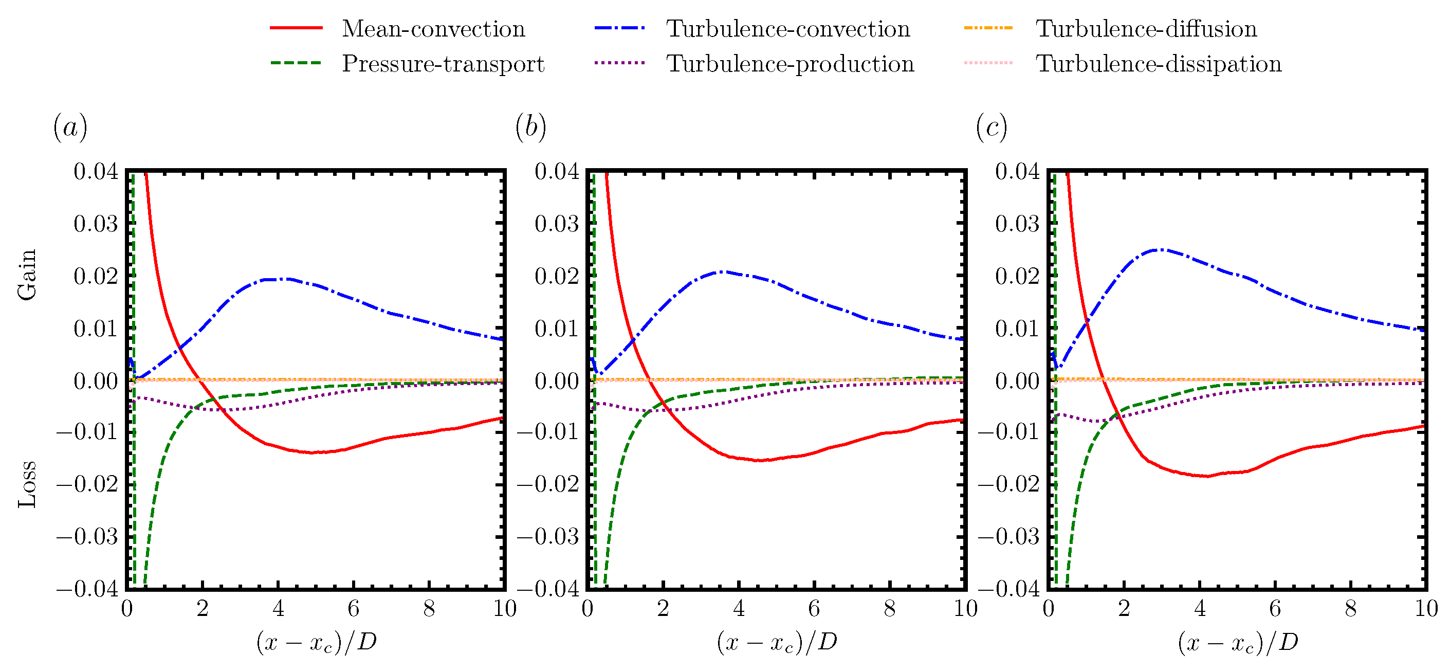
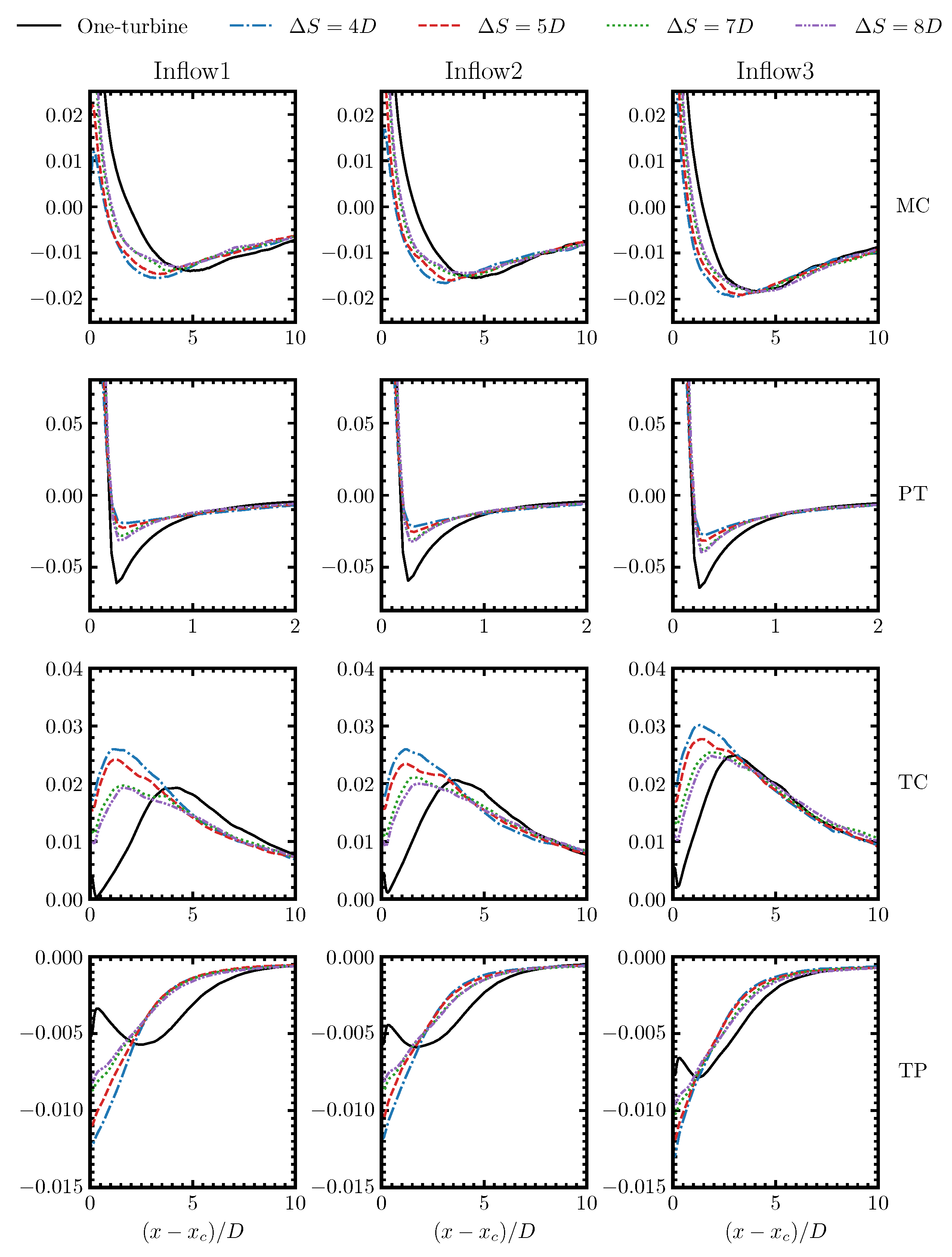
3.2. Analysis Based on the Mean Kinetic Energy Equation

To further understand the wake dynamics in various cases, in this section we analyze different terms in the mean kinetic energy (MKE) equation, which can be derived by multiplying the time-averaged momentum equation with the mean velocity, and is formulated as follows:
u i u i / 2 t = u j u i u i / 2 x j x j 1 ρ p u j + u i u j u i 2 v + v t S i j u i + u i u j u i x j 2 v + v t S i j u i x j
Considering that this is a statistically steady problem, the term on the left hand side can be eliminated. The various terms on the right hand side of the above equation are in the order they appear: (1) the change of MKE due to mean convection; (2) the diffusion term composed of transport terms due to mean pressure, Reynolds stresses, molecular and eddy viscosity; (3) the turbulence production term; and (4) the dissipation term. Equation (3) is a differential equation, which is satisfied everywhere in the flow field. In order to figure out how different terms affect the MKE in the wake region, we integrate Equation (3) from y 1 = y c R to y 2 = y c + R and z 1 = z c R to z 2 = z c + R in the spanwise and vertical directions, respectively, that the four edges of the square defined by the four points approximately enclose the wake with R = D / 2 . The obtained MKE equation in integral form is given as follows:
0 = M C + P T + T C + D F + T P + D P ,
where M C , P T , T C , T P , D F and D P denote the mean convection, pressure transport, turbulent convection, turbulence production, diffusion and dissipation terms, respectively, with their forms given as follows:
M C = y 1 y 2 z 1 z 2 u j u i u i / 2 x j d z d y , P T = y 1 y 2 z 1 z 2 p u j / ρ x j d z d y , T C = y 1 y 2 z 1 z 2 u i u j u i x j d z d y , D F = 2 y 1 y 2 z 1 z 2 v + v t S i j u i x j d z d y , T P = y 1 y 2 z 1 z 2 u i u j u i x j d z d y , D P = 2 y 1 y 2 z 1 z 2 v + v t S i j u i x j d z d y .
We first examine different terms in the MKE budget equation for the stand-alone turbine case in Figure 11, from which an intuitive impression on the relative magnitudes of different terms can be obtained. It is seen that in the near wake region, the MC term is balanced by the PT term as the pressure recovers toward the ambient pressure by extracting MKE from the wake. At further downwind locations, however, the effects of pressure transport in the MKE budget diminish rapidly and essentially approach zero for distances greater than 3 D . In this far wake region, the MC term becomes negative and is balanced by the TC term. Due to the high Reynolds number effect, the DF and DP terms are negligible compared to other terms, so we will leave it behind in the following analysis. The TP term only occupies a small part in the MKE budget, but it has significant effect on the generation of turbulence kinetic energy, which transfers the energy from the mean flow to turbulence. For the MKE budgets from cases with different ambient turbulence, the streamwise variations are very similar to each other for all the terms. By examining them more carefully, it is seen that the peak of the TC term moves upwind (from x 4 D for inflow1 to x 3 D for inflow2) with the increase of the ambient turbulence intensity. Meanwhile, the location where the MC term changes from positive to negative is found to move closer to the turbine when increasing the ambient turbulence intensity. As for the magnitudes of the peaks of the TC and TP terms, it is observed that they gradually increase when increasing the ambient turbulence intensity. The above observations indicate that increasing the ambient turbulence accelerates wake recovery as a result of the increase in turbulence convection as we can expect.
We then examine how turbine spacings affect the contributions of the MC, PT, TC and TP terms for different inflows in Figure 12. In Figure 12, all terms are set in the range of x x c = 0 10 D , except for the PT term, which changes rapidly in the near wake ( x x c = 0 2 D ). In general, it is seen that the magnitudes of different MKE budget terms in the wake of second turbine from the two-turbine case are closer to those from the corresponding stand-alone turbine case at far wake location ( x > 4 D for the MC term, x > 3 D for the TC term, x > 6 D for the TP term, respectively) when the the ground roughness length is high (for inflow3). In the near wake, the MC term is lower for the cases with Δ S = 4 D , 5 D when compared with those with Δ S = 7 D , 8 D and the stand-alone turbine case because of the relatively lower incoming wind speed when the turbine spacing is smaller. For the PT term, it is observed that the magnitude of the peak in the wake of the second turbine from the two-turbine case is significantly lower than that of the stand-alone turbine’s wake. Smaller turbine spacing leads to the PT term of lower magnitude in the near wake. One interesting observation is that the locations for the peak of the PT term are approximately the same for cases with different turbine spacings and different inflows. Interesting trends were also observed for the TC term. For the stand-alone turbine cases, it is seen that peak of the TC term moves from 4 D to 3 D turbine downwind with the normalized magnitude increasing from approximately 0.02 to 0.025 when the inflow is changed from inflow1 to inflow3. For the waked turbine, on the other hand, the peak of the TC term is located closer to the turbine, which is about 1 D and 1.5 D turbine downwind for Δ S = 4 D , 5 D and Δ = 7 D , 8 D , respectively. As for the magnitudes of the the TC term, those from the cases with Δ S = 4 D , 5 D are higher than, while those from the cases Δ S = 7 D , 8 D are similar to that from the stand-alone turbine case, respectively. That in the near wake region ( x < 3 D ) the magnitudes of the TC terms in the wake of the waked turbine are higher than those of the stand-alone turbine, explains the faster wake recovery of the waked turbine observed in Figure 9. Similar to the TC term, with the increase of the ambient turbulence intensity, the magnitude of the peak of the TP term increases with its location moving closer to the turbine (from approximately 1.5 D to 1 D turbine downwind when the inflow is changed from inflow1 to inflow3). For the waked turbine in the two-turbine case, on the other hand, the peaks of the TP term are located immediately downwind of the turbine, which is different from the stand-alone turbine case.

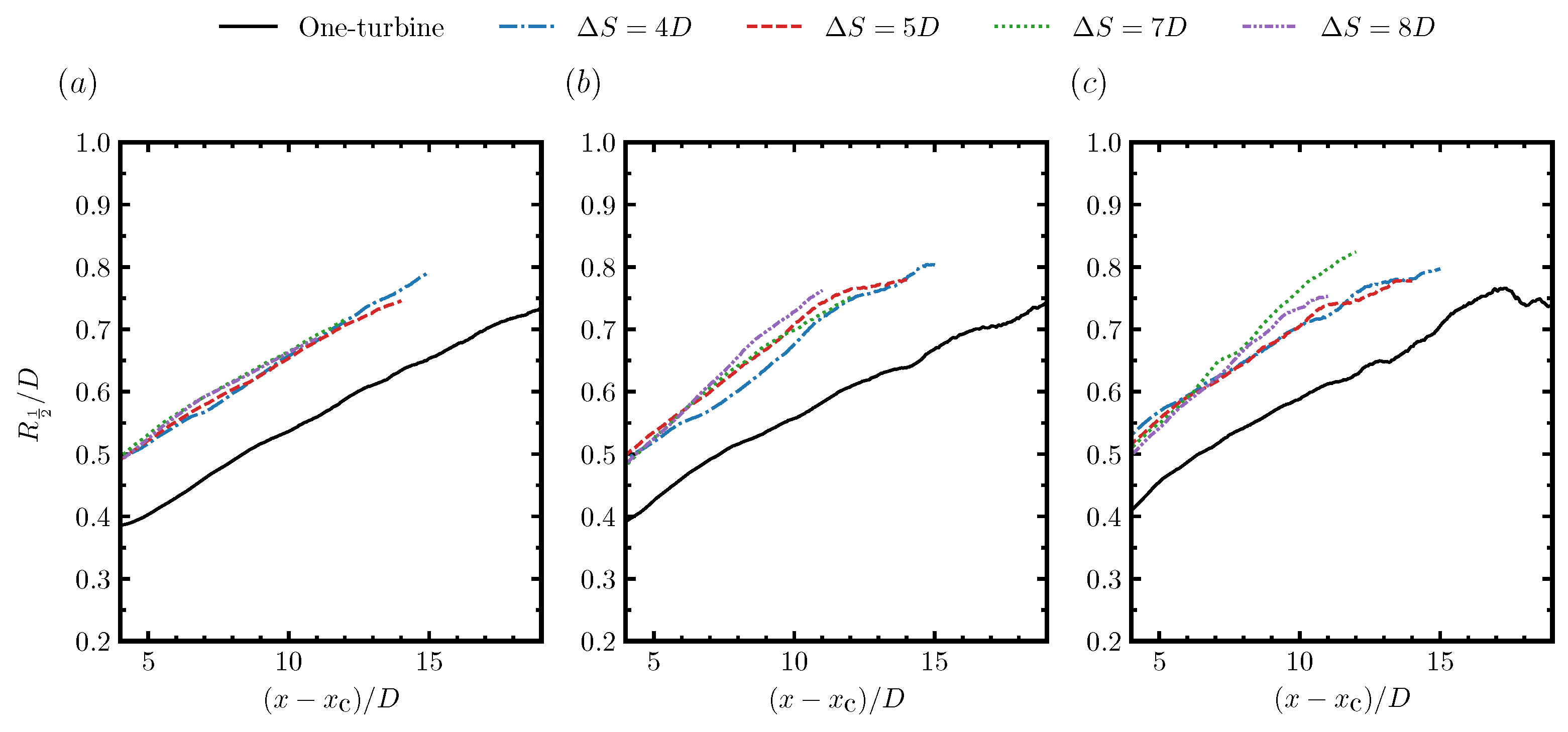
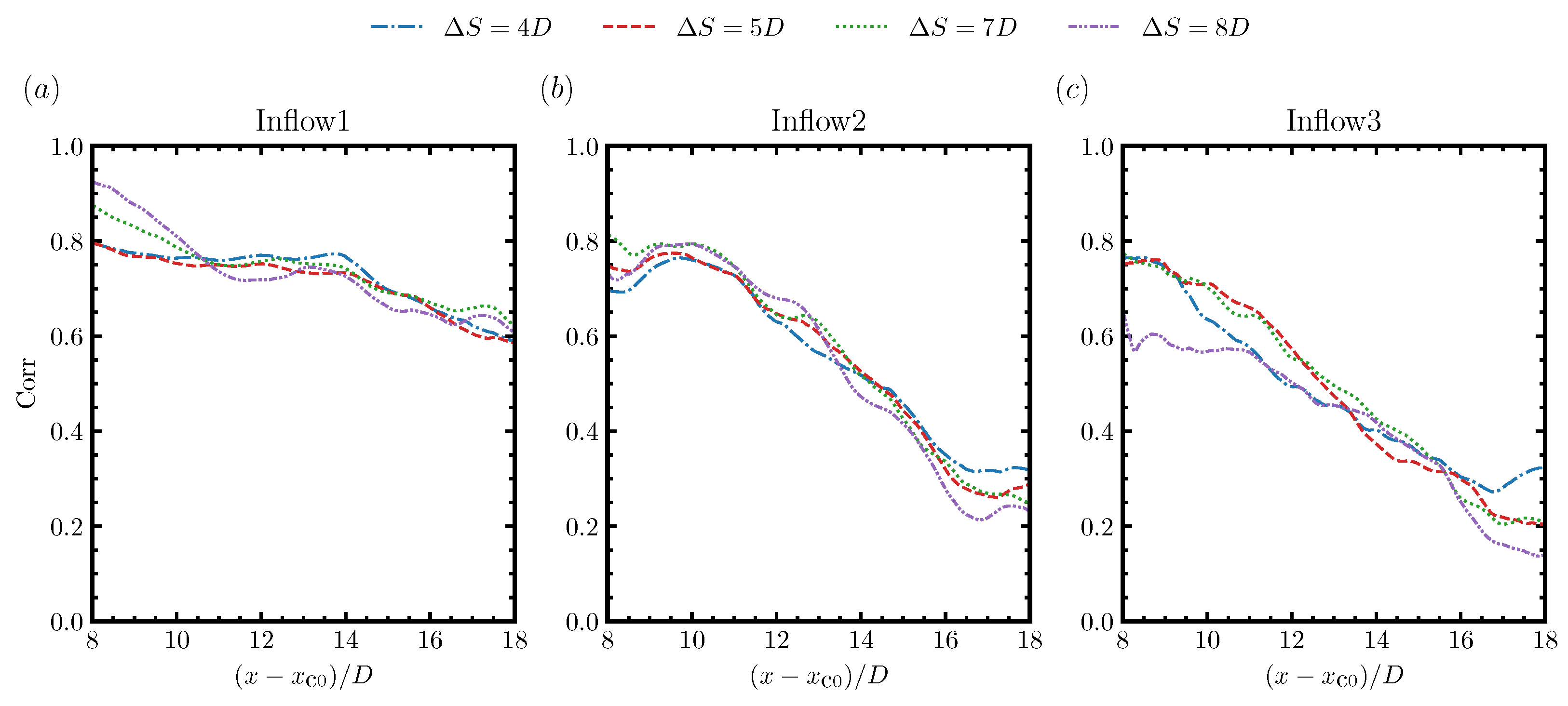
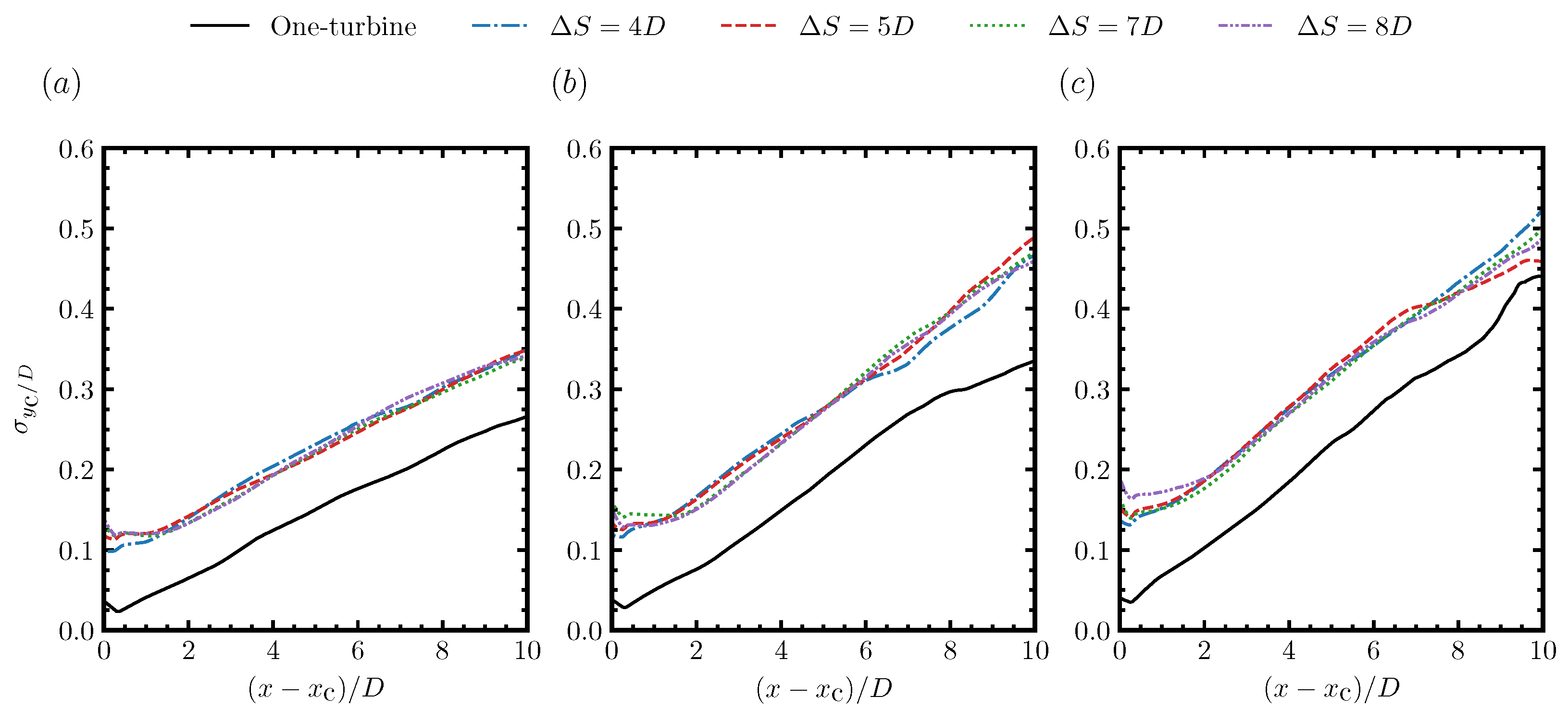
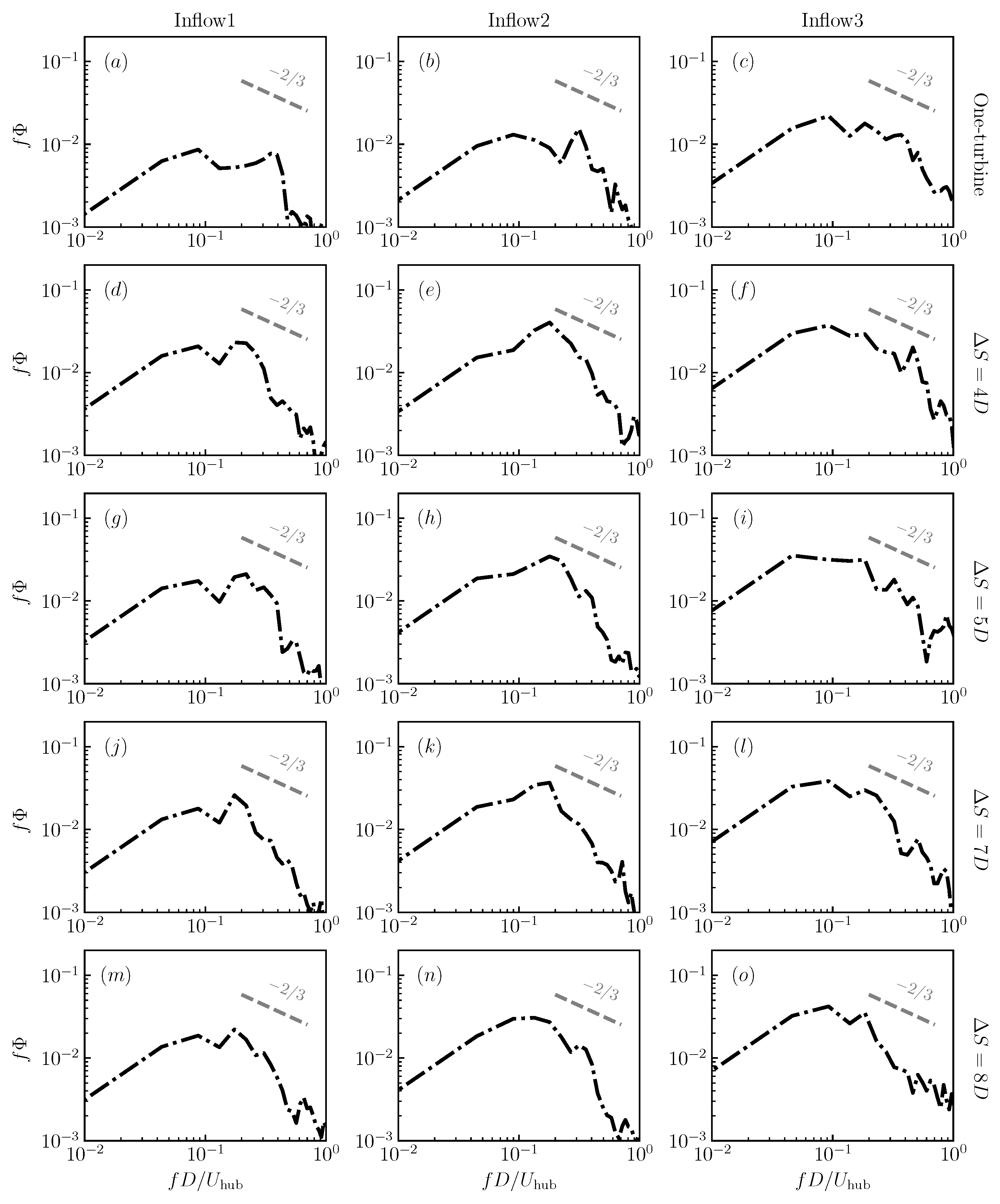
3.3. Statistics of Instantaneous Wake Positions

After analyzing the statistics of time-averaged wakes, in this section we focus on the features of the instantaneous wakes. In Figure 13, we examine the standard deviation of the instantaneous wake center positions in the spanwise direction. The instantaneous wake center was identified using the Gaussian fitting method, as in our previous work [43]. First, it is seen that the standard deviations of the instantaneous wake center positions (i.e., σ y C ) varied linearly with the downwind distance from the turbine. The growth rates of the waked turbine were approximately the same as that of the corresponding stand-alone wind turbine. With the increase of the ambient turbulence intensity, the growth rate of σ y C increased from 0.24 for inflow1, to 0.32 for inflow2 and 0.42 for inflow3. For the waked wind turbine, an overall shift of σ y C was observed, which is in the order of 0.1 D , and is approximately the same for different downwind spacings and different inflows. In the far wake, σ y C continued to increase in a linear manner, which indicates the passive scalar nature of the wake meandering for the considered cases.
We have seen that the streamwise variations of σ y C from the cases with different turbine spacings were fairly similar with each other for the same inflow. In the following, we examine how the instantaneous spanwise wake center of the waked wind turbine is correlated with that of the stand-alone wind turbine at the same streamwise locations in Figure 14. Since the horizontal coordinate was set with respect to the streamwise location of the first turbine (the same with that of the stand-alone wind turbine), ( x x c 0 ) / D = 8 would be the 4 D downwind of the second wind turbine for Δ S = 4 D , and be the position of the second wind turbine for Δ S = 8 D , respectively. It was seen that the correlations of the instantaneous spanwise wake centers of the waked turbine with the stand-alone wind turbine were very similar with each other for different turbine spacings, when the inflow was the same. For the inflow1 cases, the correlation stayed higher than approximately 0.75 for ( x x c 0 ) / D 14 , and gradually decreased to approximately 0.6 at ( x x c 0 ) / D = 18 . For the inflow2 cases, the region with high correlations became shorter, ending at ( x x c 0 ) / D 11 , and gradually decreasing to approximately 0.2 at ( x x c 0 ) / D = 17 . For the inflow3 cases, the correlation started to decrease from ( x x c 0 ) / D 9 , and decreased to 0.2 at ( x x c 0 ) / D = 17 , except for Δ S = 8 D , which stayed fairly the same in its near wake until ( x x c 0 ) / D = 11 .
The power spectral density (PSD) of the instantaneous wake positions in the spanwise direction is shown in Figure 15. Overall, it was observed that the most energetic meandering motions happened with the Strouhal number S t = f D / U h u b in the range of 0.04 0.4 . For the cases under inflow1, the motion with the maximum energy was observed around S t = 0.1 , with the other peak located around S t = 0.4 for the stand-alone wind turbine. For the waked turbines under inflow1, the peak of PSD located around S t = 0.1 persisted, while the highest peak was found near S t = 0.2 for all the considered turbine spacings. For the stand-alone wind turbine under inflow2, two noticeable peaks were observed near S t = 0.1 and 0.3 , respectively. For the waked turbine with Δ S = 4 D , 5 D , 7 D , one dominant peak was observed near S t = 0.2 , which is close to S t = 0.1 for the case with Δ S = 8 D . For the cases under inflow3, the most dominant peak of PSD was observed near S t = 0.1 , with the second dominant peak observed close to S t = 0.2 . In general, the results show that the dominant meandering frequencies from waked turbines with different turbine spacings were fairly similar with each other. Certain differences were observed between the stand-alone turbine and the waked turbine under the same inflow. The peak frequencies changed with inflows, but still fell into a similar range, i.e., S t = 0.1 0.2 . As for the PSD magnitude, it increased with the increase of the inflow turbulence intensity for the stand-alone wind turbine cases. For the cases under the same inflow, the PSD magnitude from the waked wind turbine was significantly higher than that of the stand-alone wind turbine. With the change of turbine spacings, the PSD magnitudes were fairly the same with each other.

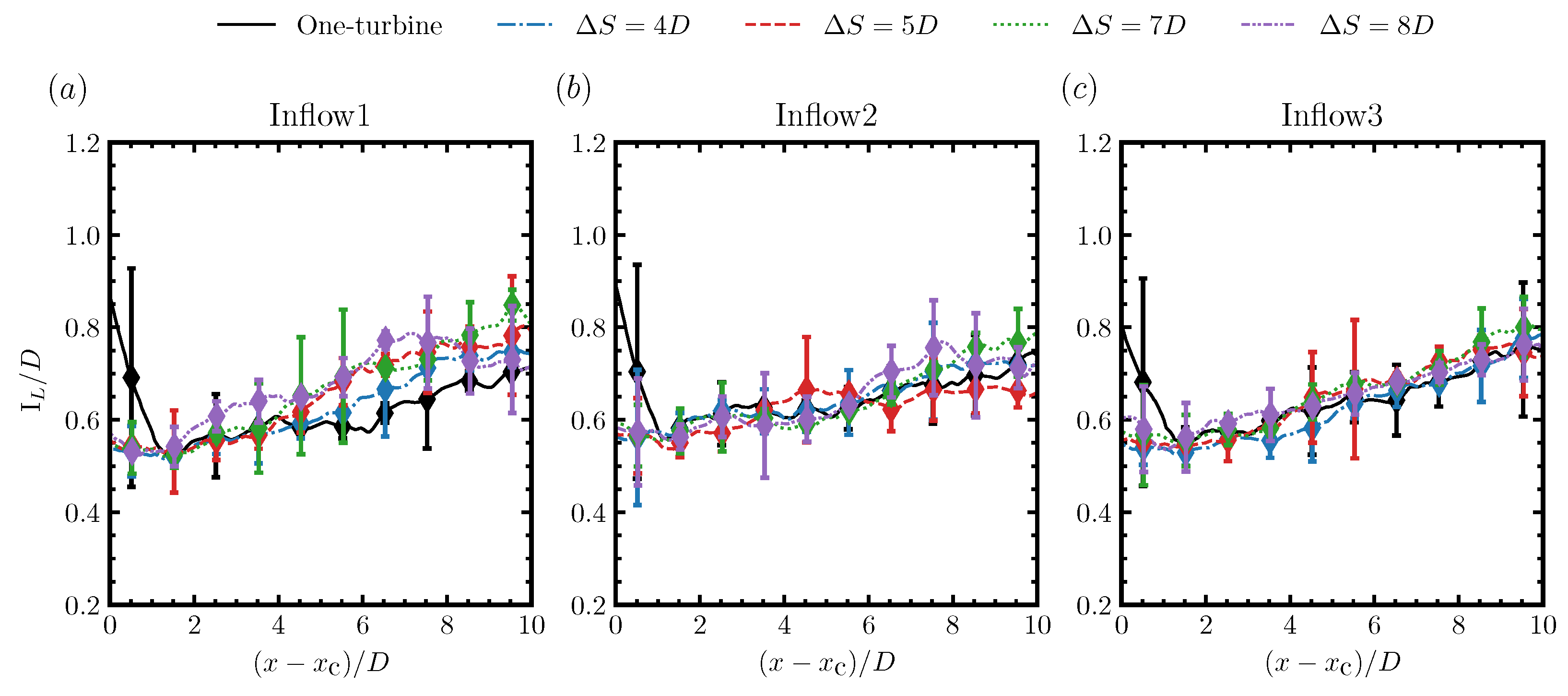
3.4. Integral Length Scale in the Wakes of the Waked Wind Turbine

In this section, we examine the integral length scale in the wake using the streamwise velocity fluctuations. First, the time correlation of the streamwise velocity fluctuation is computed as follows:
R u ( τ ) = u ( t ) u ( t + τ ) u ( τ ) 2 .
Then, the integral time scale I T is defined using the time when the auto-correlation function drops to 0.5. With the computed integral time scale, the integral length scale is estimated by multiplying the integral time scale with the local time-averaged streamwise velocity as follows:
I L = u I T
The integral length scales computed based on the above approach are shown in Figure 16. First, it was observed that in the near wake, the length scale of the stand-alone wind turbine behaved significantly different with the waked turbine, where the hub vortex in the wake of the nacelle dominates, which, however, quickly broke down for the waked turbine as a result of the oncoming wake turbulence. Downwind of this near-wake region, the integral length scale gradually increased with distance from the turbine. Overall, the integral length scales from cases with different downwind spacings were close to each other and similar to that from the corresponding stand-alone turbine. For the cases under inflow1, the integral length scales at far wake locations were more scattered, and became less scattered when the inflow was changed from inflow1 to inflow2 and inflow3.

4. Discussions

After presenting all the results from the simulated cases, in this section, we attempt to address the three questions, which were raised up in the introduction section, on how the oncoming wake turbulence affects the wake characteristics of the waked wind turbine.
Will the oncoming wake turbulence increase the wake recovery in the same way as the atmospheric turbulence? The answer is, the oncoming wake turbulence accelerates the wake recovery in a way different from the atmospheric turbulence. The difference mainly lies on the region where it plays a significant role. Compared with that from the stand-alone wind turbine, the enhanced wake recovery for the wake of a waked wind turbine mainly happens in the near wake region (Figure 9), where the increase of turbulent convection is observed from the analysis based on the MKE equation (Figure 12), enhancing the momentum mixing of the wake with the ambient flow. The atmospheric turbulence, on the other hand, affects the wake recovery until the far wake region, that the velocity deficits from the cases with higher inflow turbulence intensity are lower at far wake locations (Figure 9).
How does the oncoming wake turbulence affect the wake turbulence of the waked turbine? Similar with its effects on the wake recovery, the effect of the oncoming wake turbulence on the wake turbulence of a waked turbine is located in the near wake region (Figure 9), where the turbulence kinetic energy in the wakes of a waked turbine is higher than that of a stand-alone wind turbine. However, the integral length scale of turbulence in the very near wake region are significantly smaller for the wake of a waked turbine when compared with that of the stand-alone wind turbine (Figure 16), explaining the observation that the turbulence downwind of the waked turbine starts to decay earlier, as shown by the downwind variations of the turbulence kinetic energy (Figure 9).
Will the oncoming wake turbulence enhance the wake meandering of the waked wind turbine? The meandering of the oncoming wake initiates the wake meandering of the waked turbine as early as in its immediate downwind location, with the meandering amplitude as well as the magnitudes of PSD higher than those of the stand-alone wind turbine (Figure 13), indicating that the oncoming wake turbulence can enhance the wake meandering of the waked wind turbine. On the other hand, the downstream evolution of the wake meandering of the waked wind turbine seems to be governed by the same mechanism as that for the stand-alone wind turbine, supported by the facts that the growth rates of the meandering amplitude of the waked wind turbine are approximately the same with that of the stand-alone wind turbine (Figure 13), and the strong correlation between the instantaneous wake center locations of the waked wind turbine and those of the stand-alone wind turbine (Figure 14). This suggests that the atmospheric turbulence plays a critical role on the dynamics of wake meandering for both waked and stand-alone wind turbines.

5. Conclusions

In this work, we investigated the wake dynamics of a waked wind turbine in the configuration of two aligned wind turbines for different turbine spacings and different inflows. The 2.5 MW Eolos wind turbine was employed. Four different turbine spacings, i.e., Δ S = 4 D , 5 D , 7 D , 8 D , were considered for three different inflows, i.e., inflow1, inflow2 and inflow3 corresponding to k 0 = 0.001 , 0.01 , 0.1 m, respectively.
The statistics of the time-averaged wake were examined and compared with that of the stand-alone wind turbine under the same inflow. The simulation results show that the oncoming wake has influential effects on the near wake of the waked wind turbine. In the near wake region, it is observed that the shape of the velocity deficit at 1 D turbine downwind is closer to the Gaussian distribution compared to the double Gaussian observed in the wake of the stand-alone wind turbine. Furthermore, the magnitudes of the Reynolds shear stress and turbulence kinetic energy are significantly higher than that of the stand-alone wind turbine until approximately 4 D turbine downwind. At further downwind locations, the velocity deficits, Reynolds stresses and the turbulence kinetic energy from cases with different turbine spacings are approximately the same with each other, and close to those of the stand-alone wind turbine. The half width of the time-averaged wake is found to be increased by approximately 0.1 D for the waked turbine when compared with the stand-alone wind turbine, and increases at nearly the same rate as that of the stand-alone wind turbine as one travels downwind, especially for inflow1. The budget equation for the mean kinetic energy was further examined for different cases. The magnitudes of the turbulence convection term and turbulence production term are observed as being significantly larger in the near wake region, which explains that the oncoming wake accelerates the wake recovery and increases the turbulence kinetic energy via the increase of turbulence convection and turbulence production terms, respectively.
The statistics of the instantaneous wakes were then examined. The standard deviations of the instantaneous spanwise wake center positions from the waked turbine σ y c are plotted and compared with the stand-alone wind turbine. The simulation results show that the growth rate of σ y c in the turbine downwind direction (x) increases with the increase of the ambient turbulence intensity. For the waked wind turbine, it is seen that the streamwise variations of σ y c from cases with different downwind spacings are approximately the same with each other, and has the same slope ( σ y c via x) with the stand-alone wind turbine. To further probe into how the wake meandering of the waked turbine is correlated with that of the stand-alone wind turbine. The correlation of the instantaneous spanwise wake center position between the waked turbine and the stand-alone turbine was examined. The results show that the correlations are approximately the same for different turbine spacings, and stay around a high value for a certain range of downwind locations, which is longer for the cases with lower ambient turbulence intensity. As for the power spectral density of the instantaneous spanwise wake positions, the Strouhal numbers of the dominant frequencies from the waked turbines with different turbine spacings are in the range of 0.1 0.2 , being similar with each other, with differences observed for different inflows. The magnitudes of the power spectral density of the waked turbine, which are similar for different turbine spacings, are observed being higher than that of the stand-alone wind turbine, indicating that the oncoming wake turbulence can enhance the wake meandering of the waked wind turbine. To further explore the role of the oncoming wakes, the integral length scale along the wake centerline is plotted. It is seen that the integral length scale of the turbulence structures in wind turbine wake is smaller than one rotor diameter, which is not large enough to convect wakes as passive scalars. Furthermore, the integral length scales for the waked turbine are found to be similar with the stand-alone wind turbine. The above observations suggest that the atmospheric turbulence plays a critical role on the dynamics of wake meandering for both stand-alone and waked wind turbines for the simulated cases.
The present study provides new insights on how the oncoming wake turbulence affects the wake dynamics of waked wind turbines. The findings can be employed to develop engineering models for better including these effects in the optimization of wind farm performance. One major limitation is that this work was focused on relatively simple setups with two tandem-aligned wind turbines, without considering partial wakes, cumulative effects of upstream wakes or the wake-atmosphere interactions, which need to be considered in future work. In addition to considering more complex setups, further study on how the atmospheric turbulence affects wake meandering in the presence of complex wake-wake interactions is needed.

Author Contributions

Conceptualization, X.Y. and X.L.; methodology, X.Y., Z.L. and X.L.; software, X.Y.; verification and validation, X.L.; formal analysis, X.L.; investigation, X.L.; writing—original draft preparation, X.L.; writing—review and editing, X.Y., X.L., Z.L., D.X., S.K. and A.K.; visualization, X.L.; supervision, X.Y. All authors have read and agreed to the published version of the manuscript.

Funding

This work was supported by the NSFC Basic Science Center Program for “Multiscale Problems in Nonlinear Mechanics” (NO. 11988102), the National Natural Science Foundation of China (NO. 12172360), the Institute of Mechanics CAS and the Chinese Academy of Sciences.

Institutional Review Board Statement

Not applicable.

Informed Consent Statement

Not applicable.

Data Availability Statement

Not applicable.

Conflicts of Interest

The authors declare no conflict of interest.

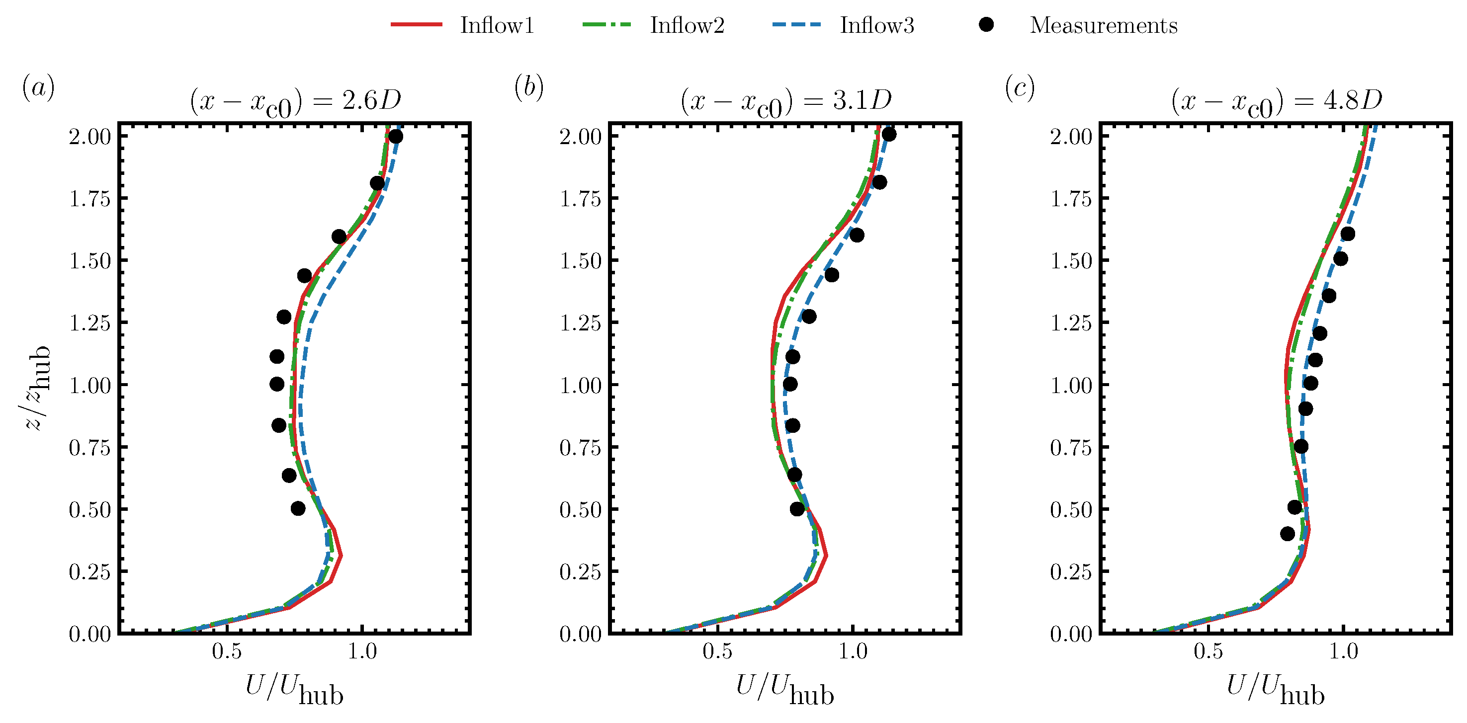
Appendix A. Validation of the Employed Method in Predicting the Wake of the Eolos Wind Turbine

The employed method has been systematically validated using both laboratory experiments and field measurements [62,70,71]. For the Eolos wind turbine simulated in this work, the capability of the employed actuator surface model in predicting its coherent tip vortices was evaluated using the super-large-scale particle image velocimetry with snow flakes as tracing particles [7]. In this appendix, we compare our simulation results with the field data collected at relatively far wake locations of the Eolos turbine at the Eolos Wind Research station, University of Minnesota [17]. Wind data were collected from five deployments located at five different turbine downwind locations, i.e., 1.8 D , 2.6 D , 3.1 D , 4.8 D and 5.1 D . For the deployment at the 1.8 D turbine downwind, the data from the met tower in the field were employed as only three data points available across the rotor plane. For the deployment at the 5.1 D turbine downwind, the incoming wind speed is higher than the rated wind speed that the turbine is operating in regime three, different from the present work. Considering these reasons, we make the comparisons between the simulations results and measurements at 2.6 D , 3.1 D and 4.8 D turbine downwind.
In the field deployments, although the Windcube for measuring wind speed was located in the wake of the Eolos turbine during most of the time period, the wind direction did vary during the data collection. In the simulations, on the other hand, the wind direction was fixed. To account for such differences between the simulations and measurements, the vertical profiles of the streamwise velocity are averaged at several spanwise locations instead of running several cases with different wind directions, considering that the change of wind direction is equivalent to the variation of the relative position of the measuring point in the wake. Specifically, we equally divide the range of the absolute wind direction angle (the wake is nearly symmetry in the spanwise direction) into four intervals, and obtain the mean streamwise velocity by averaging over the four intervals with their weights computed based on the time series of the wind direction shown in [17].
The obtained vertical profiles of the mean streamwise velocity from the simulations are compared with the field measurements in Figure A1. One can observe that predictions from the simulations agree fairly well with the field measurements for all three turbine downwind locations.
Figure A1. Comparison of the vertical profile of the mean streamwise velocity between the simulations and the field measurements at 2.6 D (a), 3.1 D (b), 4.8 D (c) turbine downwind locations.
Energies 15 02899 g0a1

References

  1. Barthelmie, R.J.; Jensen, L. Evaluation of wind farm efficiency and wind turbine wakes at the Nysted offshore wind farm. Wind Energy 2010, 13, 573–586. [Google Scholar] [CrossRef]
  2. Stevens, R.J.; Meneveau, C. Flow structure and turbulence in wind farms. Annu. Rev. Fluid Mech. 2017, 49, 311–339. [Google Scholar] [CrossRef]
  3. Vermeer, L.; Sørensen, J.N.; Crespo, A. Wind turbine wake aerodynamics. Prog. Aerosp. Sci. 2003, 39, 467–510. [Google Scholar] [CrossRef]
  4. Chen, G.; Li, X.B.; Liang, X.F. IDDES Simulation of the Performance and Wake Dynamics of the Wind Turbines under Different Turbulent Inflow Conditions. Energy 2022, 238, 121772. [Google Scholar] [CrossRef]
  5. Dasari, T.; Wu, Y.; Liu, Y.; Hong, J. Near-Wake Behaviour of a Utility-Scale Wind Turbine. J. Fluid Mech. 2019, 859, 204–246. [Google Scholar] [CrossRef]
  6. Na, J.S.; Koo, E.; Ko, S.C.; Linn, R.; Muñoz-Esparza, D.; Jin, E.K.; Lee, J.S. Stochastic Characteristics for the Vortical Structure of a 5-MW Wind Turbine Wake. Renew. Energy 2019, 133, 1220–1230. [Google Scholar] [CrossRef]
  7. Yang, X.; Hong, J.; Barone, M.; Sotiropoulos, F. Coherent dynamics in the rotor tip shear layer of utility-scale wind turbines. J. Fluid Mech. 2016, 804, 90–115. [Google Scholar] [CrossRef] [Green Version]
  8. Hong, J.; Toloui, M.; Chamorro, L.P.; Guala, M.; Howard, K.; Riley, S.; Tucker, J.; Sotiropoulos, F. Natural snowfall reveals large-scale flow structures in the wake of a 2.5-MW wind turbine. Nat. Commun. 2014, 5, 4216. [Google Scholar] [CrossRef]
  9. Larsen, G.C.; Madsen, H.A.; Mann, J.; Ott, S.; Sørensen, J.N.; Okulov, V.; Troldborg, N.; Nielsen, M.; Thomsen, K.; Larsen, T.J. Dynamic Wake Meandering Modeling; Tech Note Risø-M-1607; Risoe National Lab.: Roskilde, Denmark, 2007; p. 85. [Google Scholar]
  10. Yang, X.; Sotiropoulos, F. Wake characteristics of a utility-scale wind turbine under coherent inflow structures and different operating conditions. Phys. Rev. Fluids 2019, 4, 024604. [Google Scholar] [CrossRef]
  11. Medici, D.; Alfredsson, P. Measurements on a wind turbine wake: 3D effects and bluff body vortex shedding. Wind Energy 2006, 9, 219–236. [Google Scholar] [CrossRef]
  12. Kang, S.; Yang, X.; Sotiropoulos, F. On the onset of wake meandering for an axial flow turbine in a turbulent open channel flow. J. Fluid Mech. 2014, 744, 376–403. [Google Scholar] [CrossRef]
  13. Trujillo, J.J.; Bingöl, F.; Larsen, G.C.; Mann, J.; Kühn, M. Light detection and ranging measurements of wake dynamics. Part II: Two-dimensional scanning. Wind Energy 2011, 14, 61–75. [Google Scholar] [CrossRef]
  14. Foti, D.; Yang, X.; Guala, M.; Sotiropoulos, F. Wake meandering statistics of a model wind turbine: Insights gained by large eddy simulations. Phys. Rev. Fluids 2016, 1, 044407. [Google Scholar] [CrossRef]
  15. Foti, D.; Yang, X.; Campagnolo, F.; Maniaci, D.; Sotiropoulos, F. Wake meandering of a model wind turbine operating in two different regimes. Phys. Rev. Fluids 2018, 3, 054607. [Google Scholar] [CrossRef]
  16. Brugger, P.A.; Markfort, C.D.; Porté-Agel, F. Field Measurements of Wake Meandering at a Utility-Scale Wind Turbine with Nacelle-Mounted Doppler LiDARs. Wind Energy Sci. Discuss. 2021, 7, 185–199. [Google Scholar] [CrossRef]
  17. Heisel, M.; Hong, J.; Guala, M. The spectral signature of wind turbine wake meandering: A wind tunnel and field-scale study. Wind Energy 2018, 21, 715–731. [Google Scholar] [CrossRef]
  18. Chamorro, L.; Hill, C.; Morton, S.; Ellis, C.; Arndt, R.; Sotiropoulos, F. On the interaction between a turbulent open channel flow and an axial-flow turbine. J. Fluid Mech. 2013, 716, 658–670. [Google Scholar] [CrossRef]
  19. Iungo, G.V.; Viola, F.; Camarri, S.; Porté-Agel, F.; Gallaire, F. Linear stability analysis of wind turbine wakes performed on wind tunnel measurements. J. Fluid Mech. 2013, 737, 499–526. [Google Scholar] [CrossRef] [Green Version]
  20. Howard, K.B.; Singh, A.; Sotiropoulos, F.; Guala, M. On the Statistics of Wind Turbine Wake Meandering: An Experimental Investigation. Phys. Fluids 2015, 27, 075103. [Google Scholar] [CrossRef]
  21. Foti, D.; Yang, X.; Shen, L.; Sotiropoulos, F. Effect of wind turbine nacelle on turbine wake dynamics in large wind farms. J. Fluid Mech. 2019, 869, 1–26. [Google Scholar] [CrossRef]
  22. Yang, X.; Sotiropoulos, F. A review on the meandering of wind turbine wakes. Energies 2019, 12, 4725. [Google Scholar] [CrossRef] [Green Version]
  23. Uchida, T. Effects of Inflow Shear on Wake Characteristics of Wind-Turbines over Flat Terrain. Energies 2020, 13, 3745. [Google Scholar] [CrossRef]
  24. De Cillis, G.; Cherubini, S.; Semeraro, O.; Leonardi, S.; De Palma, P. POD Analysis of the Recovery Process in Wind Turbine Wakes. J. Phys. 2020, 1618, 062016. [Google Scholar] [CrossRef]
  25. Wu, Y.T.; Lin, C.Y.; Chang, T.J. Effects of Inflow Turbulence Intensity and Turbine Arrangements on the Power Generation Efficiency of Large Wind Farms. Wind Energy 2020, 23, 1640–1655. [Google Scholar] [CrossRef]
  26. Bastankhah, M.; Porté-Agel, F. Wind tunnel study of the wind turbine interaction with a boundary-layer flow: Upwind region, turbine performance, and wake region. Phys. Fluids 2017, 29, 065105. [Google Scholar] [CrossRef]
  27. Chamorro, L.P.; Porté-Agel, F. Effects of thermal stability and incoming boundary-layer flow characteristics on wind-turbine wakes: A wind-tunnel study. Bound.-Layer Meteorol. 2010, 136, 515–533. [Google Scholar] [CrossRef] [Green Version]
  28. Du, B.; Ge, M.; Zeng, C.; Cui, G.; Liu, Y. Influence of Atmospheric Stability on Wind-Turbine Wakes with a Certain Hub-Height Turbulence Intensity. Phys. Fluids 2021, 33, 055111. [Google Scholar] [CrossRef]
  29. Churchfield, M.J.; Lee, S.; Michalakes, J.; Moriarty, P.J. A numerical study of the effects of atmospheric and wake turbulence on wind turbine dynamics. J. Turbul. 2012, 13, N14. [Google Scholar] [CrossRef]
  30. Herges, T.; Berg, J.C.; Bryant, J.; White, J.; Paquette, J.; Naughton, B.T. Detailed analysis of a waked turbine using a high-resolution scanning lidar. J. Phys. 2018, 1037, 072009. [Google Scholar] [CrossRef]
  31. Yang, X.; Howard, K.B.; Guala, M.; Sotiropoulos, F. Effects of a three-dimensional hill on the wake characteristics of a model wind turbine. Phys. Fluids 2015, 27, 025103. [Google Scholar] [CrossRef]
  32. Howard, K.; Hu, J.; Chamorro, L.; Guala, M. Characterizing the response of a wind turbine model under complex inflow conditions. Wind Energy 2015, 18, 729–743. [Google Scholar] [CrossRef]
  33. Gao, X.; Wang, T.; Li, B.; Sun, H.; Yang, H.; Han, Z.; Wang, Y.; Zhao, F. Investigation of wind turbine performance coupling wake and topography effects based on LiDAR measurements and SCADA data. Appl. Energy 2019, 255, 113816. [Google Scholar] [CrossRef]
  34. Wang, J.; Mclean, D.; Campagnolo, F.; Yu, T.; Bottasso, C.L. Large-eddy simulation of waked turbines in a scaled wind farm facility. J. Phys. 2017, 854, 012047. [Google Scholar] [CrossRef] [Green Version]
  35. Bartl, J.; Pierella, F.; Sætrana, L. Wake Measurements Behind an Array of Two Model Wind Turbines. Energy Procedia 2012, 24, 305–312. [Google Scholar] [CrossRef] [Green Version]
  36. Adaramola, M.; Krogstad, P.Å. Experimental investigation of wake effects on wind turbine performance. Renew. Energy 2011, 36, 2078–2086. [Google Scholar] [CrossRef]
  37. Mycek, P.; Gaurier, B.; Germain, G.; Pinon, G.; Rivoalen, E. Experimental Study of the Turbulence Intensity Effects on Marine Current Turbines Behaviour. Part II: Two Interacting Turbines. Renew. Energy 2014, 68, 876–892. [Google Scholar] [CrossRef] [Green Version]
  38. Wu, C.; Yang, X.; Zhu, Y. On the design of potential turbine positions for physics-informed optimization of wind farm layout. Renew. Energy 2021, 164, 1108–1120. [Google Scholar] [CrossRef]
  39. Xie, S.; Archer, C. Self-similarity and Turbulence Characteristics of Wind Turbine Wakes via Large-eddy Simulation. Wind Energy 2015, 18, 1815–1838. [Google Scholar] [CrossRef]
  40. Bastankhah, M.; Porté-Agel, F. Experimental and theoretical study of wind turbine wakes in yawed conditions. J. Fluid Mech. 2016, 806, 506–541. [Google Scholar] [CrossRef]
  41. Li, L.; Huang, Z.; Ge, M.; Zhang, Q. A Novel Three-Dimensional Analytical Model of the Added Streamwise Turbulence Intensity for Wind-Turbine Wakes. Energy 2022, 238, 121806. [Google Scholar] [CrossRef]
  42. Foti, D.; Yang, X.; Sotiropoulos, F. Similarity of wake meandering for different wind turbine designs for different scales. J. Fluid Mech. 2018, 842, 5–25. [Google Scholar] [CrossRef]
  43. Li, Z.; Yang, X. Large-Eddy Simulation on the Similarity between Wakes of Wind Turbines with Different Yaw Angles. J. Fluid Mech. 2021, 921, A11. [Google Scholar] [CrossRef]
  44. Katic, I.; Højstrup, J.; Jensen, N.O. A simple model for cluster efficiency. In Proceedings of the European Wind Energy Association Conference and Exhibition, Rome, Italy, 7–9 October 1986; pp. 407–410. [Google Scholar]
  45. Calaf, M.; Meneveau, C.; Meyers, J. Large eddy simulation study of fully developed wind-turbine array boundary layers. Phys. Fluids 2010, 22, 015110. [Google Scholar] [CrossRef] [Green Version]
  46. Yang, X.; Sotiropoulos, F. Analytical model for predicting the performance of arbitrary size and layout wind farms. Wind Energy 2016, 19, 1239–1248. [Google Scholar] [CrossRef]
  47. Ge, M.; Wu, Y.; Liu, Y.; Li, Q. A two-dimensional model based on the expansion of physical wake boundary for wind-turbine wakes. Appl. Energy 2019, 233, 975–984. [Google Scholar] [CrossRef]
  48. Yang, X.; Kang, S.; Sotiropoulos, F. Computational study and modeling of turbine spacing effects in infinite aligned wind farms. Phys. Fluids 2012, 24, 115107. [Google Scholar] [CrossRef]
  49. Moon, J.S.; Manuel, L. Toward understanding waked flow fields behind a wind turbine using proper orthogonal decomposition. J. Renew. Sustain. Energy 2021, 13, 023302. [Google Scholar] [CrossRef]
  50. Shaler, K.; Debnath, M.; Jonkman, J. Validation of FAST.farm against full-scale turbine SCADA data for a small wind farm. J. Phys. 2020, 1618, 062061. [Google Scholar] [CrossRef]
  51. Yang, X. Towards the development of a wake meandering model based on neural networks. J. Phys. 2020, 1618, 062026. [Google Scholar] [CrossRef]
  52. Porté-Agel, F.; Bastankhah, M.; Shamsoddin, S. Wind-turbine and wind-farm flows: A review. Bound.-Layer Meteorol. 2020, 174, 1–59. [Google Scholar] [CrossRef] [Green Version]
  53. Zong, H.; Porté-Agel, F. A Momentum-Conserving Wake Superposition Method for Wind Farm Power Prediction. J. Fluid Mech. 2020, 889, A8. [Google Scholar] [CrossRef]
  54. Lanzilao, L.; Meyers, J. A New Wake-merging Method for Wind-farm Power Prediction in the Presence of Heterogeneous Background Velocity Fields. Wind Energy 2021, 25, 237–259. [Google Scholar] [CrossRef]
  55. Porté-Agel, F. Interaction between Large Wind Farms and the Atmospheric Boundary Layer. Procedia IUTAM 2014, 10, 307–318. [Google Scholar] [CrossRef] [Green Version]
  56. Fleming, P.; Gebraad, P.M.; Lee, S.; van Wingerden, J.W.; Johnson, K.; Churchfield, M.; Michalakes, J.; Spalart, P.; Moriarty, P. Simulation comparison of wake mitigation control strategies for a two-turbine case. Wind Energy 2015, 18, 2135–2143. [Google Scholar] [CrossRef]
  57. Annoni, J.; Seiler, P.; Johnson, K.; Fleming, P.; Gebraad, P. Evaluating wake models for wind farm control. In Proceedings of the 2014 American Control Conference, Portland, OR, USA, 4–6 June 2014; pp. 2517–2523. [Google Scholar]
  58. Boersma, S.; Doekemeijer, B.M.; Gebraad, P.M.; Fleming, P.A.; Annoni, J.; Scholbrock, A.K.; Frederik, J.A.; van Wingerden, J.W. A tutorial on control-oriented modeling and control of wind farms. In Proceedings of the 2017 American Control Conference (ACC), Seattle, WA, USA, 24–26 May 2017; pp. 1–18. [Google Scholar]
  59. Fleming, P.; Aho, J.; Gebraad, P.; Pao, L.; Zhang, Y. Computational fluid dynamics simulation study of active power control in wind plants. In Proceedings of the 2016 American Control Conference (ACC), Boston, MA, USA, 6–8 July 2016; pp. 1413–1420. [Google Scholar]
  60. van Wingerden, J.W.; Pao, L.; Aho, J.; Fleming, P. Active power control of waked wind farms. IFAC-PapersOnLine 2017, 50, 4484–4491. [Google Scholar] [CrossRef]
  61. Vali, M.; Petrović, V.; Boersma, S.; van Wingerden, J.W.; Pao, L.Y.; Kühn, M. Model predictive active power control of waked wind farms. In Proceedings of the 2018 Annual American Control Conference (ACC), Milwaukee, WI, USA, 27–29 June 2018; pp. 707–714. [Google Scholar]
  62. Yang, X.; Sotiropoulos, F.; Conzemius, R.J.; Wachtler, J.N.; Strong, M.B. Large-eddy simulation of turbulent flow past wind turbines/farms: The Virtual Wind Simulator (VWiS). Wind Energy 2015, 18, 2025–2045. [Google Scholar] [CrossRef]
  63. Yang, X.; Angelidis, D.; Khosronejad, A.; Le, T.; Kang, S.; Gilmanov, A.; Ge, L.; Borazjani, I.; Calderer, A. Virtual Flow Simulator; Computer Software; USDOE Office of Energy Efficiency and Renewable Energy (EERE): Washington, DC, USA, 2015. [CrossRef]
  64. Li, S.; Yang, X.; Jin, G.; He, G. Wall-resolved large-eddy simulation of turbulent channel flows with rough walls. Theor. Appl. Mech. Lett. 2021, 11, 100228. [Google Scholar] [CrossRef]
  65. Yang, X.; Khosronejad, A.; Sotiropoulos, F. Large-eddy simulation of a hydrokinetic turbine mounted on an erodible bed. Renew. Energy 2017, 113, 1419–1433. [Google Scholar] [CrossRef]
  66. Yang, X.; Sotiropoulos, F. On the dispersion of contaminants released far upwind of a cubical building for different turbulent inflows. Build. Environ. 2019, 154, 324–335. [Google Scholar] [CrossRef]
  67. Chen, Y.; Yang, X.; Iskander, A.J.; Wang, P. On the flow characteristics in different carotid arteries. Phys. Fluids 2020, 32, 101902. [Google Scholar] [CrossRef]
  68. Liao, F.; Wang, S.; Yang, X.; He, G. A simulation-based actuator surface parameterization for large-eddy simulation of propeller wakes. Ocean. Eng. 2020, 199, 107023. [Google Scholar] [CrossRef]
  69. Zhou, Z.; Li, Z.; He, G.; Yang, X. Towards multi-fidelity simulation of flows around an underwater vehicle with appendages and propeller. Theor. Appl. Mech. Lett. 2021, 12, 100318. [Google Scholar] [CrossRef]
  70. Yang, X.; Sotiropoulos, F. A new class of actuator surface models for wind turbines. Wind Energy 2018, 21, 285–302. [Google Scholar] [CrossRef] [Green Version]
  71. Yang, X.; Pakula, M.; Sotiropoulos, F. Large-eddy simulation of a utility-scale wind farm in complex terrain. Appl. Energy 2018, 229, 767–777. [Google Scholar] [CrossRef]
  72. Germano, M.; Piomelli, U.; Moin, P.; Cabot, W.H. A dynamic subgrid-scale eddy viscosity model. Phys. Fluids A 1991, 3, 1760–1765. [Google Scholar] [CrossRef] [Green Version]
  73. Yang, X.; Zhang, X.; Li, Z.; He, G.W. A smoothing technique for discrete delta functions with application to immersed boundary method in moving boundary simulations. J. Comput. Phys. 2009, 228, 7821–7836. [Google Scholar] [CrossRef]
  74. Ge, L.; Sotiropoulos, F. A numerical method for solving the 3D unsteady incompressible Navier–Stokes equations in curvilinear domains with complex immersed boundaries. J. Comput. Phys. 2007, 225, 1782–1809. [Google Scholar] [CrossRef] [Green Version]
  75. Knoll, D.A.; Keyes, D.E. Jacobian-free Newton–Krylov methods: A survey of approaches and applications. J. Comput. Phys. 2004, 193, 357–397. [Google Scholar] [CrossRef] [Green Version]
  76. Saad, Y. A flexible inner-outer preconditioned GMRES algorithm. SIAM J. Sci. Comput. 1993, 14, 461–469. [Google Scholar] [CrossRef]
  77. Mamouri, A.R.; Khoshnevis, A.B.; Lakzian, E. Experimental Study of the Effective Parameters on the Offshore Wind Turbine’s Airfoil in Pitching Case. Ocean. Eng. 2020, 198, 106955. [Google Scholar] [CrossRef]
  78. Barthelmie, R.J.; Hansen, K.; Frandsen, S.T.; Rathmann, O.; Schepers, J.; Schlez, W.; Phillips, J.; Rados, K.; Zervos, A.; Politis, E.; et al. Modelling and measuring flow and wind turbine wakes in large wind farms offshore. Wind Energy 2009, 12, 431–444. [Google Scholar] [CrossRef]
  79. Yang, X.; Milliren, C.; Kistner, M.; Hogg, C.; Marr, J.; Shen, L.; Sotiropoulos, F. High-fidelity simulations and field measurements for characterizing wind fields in a utility-scale wind farm. Appl. Energy 2021, 281, 116115. [Google Scholar] [CrossRef]
  80. Meyers, J.; Meneveau, C. Optimal turbine spacing in fully developed wind farm boundary layers. Wind Energy 2012, 15, 305–317. [Google Scholar] [CrossRef] [Green Version]
Figure 1. Schematic of the computational set-up of the simulated cases.
Energies 15 02899 g001
Figure 2. Vertical profiles of (a) mean streamwise velocity and (b) turbulence kinetic energy.
Energies 15 02899 g002
Figure 3. Power (a) and thrust (b) of the waked turbine normalized by those of the first turbine for different turbulent inflows.
Energies 15 02899 g003
Figure 4. Contours of instantaneous streamwise velocity on the horizontal plane located at turbine hub height for (a) the stand-alone turbine case and (b) the two-turbine case with Δ S / D = 4 for inflow1 with k 0 = 0.001 m.
Energies 15 02899 g004
Figure 5. Contours of instantaneous spanwise velocity on the horizontal plane located at turbine hub height for (a) the stand-alone turbine case and (b) the two-turbine case with Δ S / D = 4 for inflow1 with k 0 = 0.001 m.
Energies 15 02899 g005
Figure 6. Spanwise profiles of the streamwise velocity deficits downwind of the second turbine of the two-turbine cases and downwind of the stand-alone turbine at (a) ( x x c ) / D = 1, (b) 3, (c) 5, (d) 7, (e) 9, (f) 11.
Energies 15 02899 g006
Figure 7. Spanwise profiles of the Reynolds stress u v downwind of the second turbine of the two-turbine cases and downwind of the stand-alone turbine at (a) ( x x c ) / D = 1, (b) 3, (c) 5, (d) 7, (e) 9, (f) 11.
Energies 15 02899 g007
Figure 8. Spanwise profiles of the turbulence kinetic energy downwind of the second turbine of the two-turbine cases and downwind of the stand-alone turbine at (a) ( x x c ) / D = 1, (b) 3, (c) 5, (d) 7, (e) 9, (f) 11.
Energies 15 02899 g008
Figure 9. Streamwise variations of (a,c,e) disk-averaged streamwise velocity deficit, and (b,d,f) disk-averaged turbulence kinetic energy at different streamwise positions under different inflows.
Energies 15 02899 g009
Figure 10. Streamwise variations of the half width R 1 2 of the time-averaged wake, which is obtained by fitting the time-averaged velocity deficit using the Gaussian distribution, for (a) inflow1, (b) inflow2, and (c) inflow3, respectively.
Energies 15 02899 g010
Figure 11. Different terms in the MKE budget equation for the stand-alone turbine case under inflow1 (a), inflow2 (b) and inflow3 (c). Different terms are normalized using U hub and D.
Energies 15 02899 g011
Figure 12. Comparison of the MC, PT, TC and TP terms in the wake of the waked turbine of the two-turbine cases with the stand-alone turbine for different turbine spacings and different inflows. Different terms are normalized using U hub and D.
Energies 15 02899 g012
Figure 13. Streamwise variations of the standard deviations of the instantaneous spanwise wake centers under different inflow conditions for (a) inflow1, (b) inflow2 and (c) inflow3.
Energies 15 02899 g013
Figure 14. Correlation coefficients between the instantaneous spanwise wake positions of the waked turbine and those of the stand-alone wind turbine at different streamwise locations for (a) inflow1, (b) inflow2 and (c) inflow3, respectively.
Energies 15 02899 g014
Figure 15. Power spectral density of instantaneous spanwise wake positions at ( x x c ) / D = 5 under different inflow conditions.
Energies 15 02899 g015
Figure 16. Streamwise variations of the integral length scale computed using Equation (7) for (a) inflow1, (b) inflow2 and (c) inflow3, respectively. It is noticed that the integral length scale is filtered in the streamwise direction with the filter scale D, with the error bar showing the stand deviation of the subfilter fluctuations.
Energies 15 02899 g016
Table 1. Summary of the cases simulated in this work.
Inflow StatisticsNumber of TurbinesTurbine SpacingGrid Resolution
inflow1 k 0 = 0.001
k h u b / U h u b 2 = 0.0038
stand-alone Δ x / D = 1 / 20
Δ y / D = 1 / 40
Δ z m i n / D = 1 / 40
Δ t U h u b D 0.00178
two-turbines Δ S / D = 4 , 5 , 7 , 8
inflow2 k 0 = 0.01
k h u b / U h u b 2 = 0.0052
stand-alone
two-turbines Δ S / D = 4 , 5 , 7 , 8
inflow3 k 0 = 0.1
k h u b / U h u b 2 = 0.0081
stand-alone
two-turbines Δ S / D = 4 , 5 , 7 , 8
Publisher’s Note: MDPI stays neutral with regard to jurisdictional claims in published maps and institutional affiliations.

