
Realistic Simulation of Sensor/Actuator Faults for a Dependability Evaluation of Demand-Controlled Ventilation and Heating Systems


Department of Electrical Engineering and Computer Science, University of Siegen, 57076 Siegen, Germany
*
Author to whom correspondence should be addressed.
Energies 2022, 15(8), 2878; https://doi.org/10.3390/en15082878
Submission received: 16 February 2022
/
Revised: 16 March 2022
/
Accepted: 12 April 2022
/
Published: 14 April 2022
(This article belongs to the Special Issue Fault Identification and Fault Impact Analysis of Ventilation System in Buildings)
Abstract
:In the development of fault-tolerant systems, simulation is a common technique used to obtain insights into performance and dependability because it saves time and avoids the risks of testing the behavior of real-world systems in the presence of faults. Fault injection in a simulation offers a high controllability and observability, and thus is ideal for an early dependability analysis and fault-tolerance evaluation. Heating, ventilation, and air conditioning (HVAC) systems in critical infrastructures, such as airports and hospitals, are safety-relevant systems, which not only determine energy consumption, system efficiency, and occupancy comfort but also play an essential role in emergency scenarios (e.g., fires, biological hazards). Hence, fault injection serves as a practical and essential solution to assess dependability in different fault scenarios of HVAC systems. Hence, in this paper, we present a simulation-based fault injection framework with a combination of two techniques, simulator command and simulation code modification, which are applied to fault injector blocks as saboteurs and an automated fault injector algorithm to automatically activate fault cases with certain fault attributes. The proposed fault injection framework supports a comprehensive range of faults and various fault attributes, including fault persistence, fault type, fault location, fault duration, and fault interarrival time. This framework considers noise in a demand-controlled ventilation (DCV) and heating system as a type of HVAC system since it has been demonstrated that any fault injection scenario is accompanied by some impacts on energy consumption, occupancy comfort, and a fire risk. It also supports the reproducibility for a set of specific fault scenarios or random fault injection scenarios. The system model was implemented and simulated in Matlab/Simulink, and fault injector blocks were developed by Stateflow diagrams. An experimental evaluation serves as the assessment of the presented fault injection framework with a defined example of fault scenarios. The results of the evaluation show the correctness, system behavior, accuracy, and other parameters of the system, such as the heater energy consumption and heater duty cycle of the fault injection framework in the presence of different fault cases. In conclusion, the present paper provides a novel simulation-based fault injection framework, which combines simulator command techniques and simulation code modifications for a realistic and automatic fault injection with comprehensive coverage of various fault types and a consideration of noise and uncertainty, allowing for reproducibility of the results. The outputs achieved from the fault injection framework can be applied to fault-tolerant studies in other application domains.
1. Introduction and Literature Review
Modern smart buildings play an important role in terms of economy, ecology, and human well-being. They are equipped with various electronic components, including different actuators, sensors, and automatic control systems called building management systems (BMS) [1,2]. The user’s comfort is important and affected by the operation of heating, ventilation, and air conditioning (HVAC), which is considered to be a major source of energy consumption. The efficient operation of an HVAC system affects the efficiency of the overall system, which is the BMS [1]. In addition, many sensors and actuators are integrated with an HVAC system, and the interactions of these components are fault-prone. Without fault-tolerant techniques, the system may face unpredictable conditions. Therefore, a dependability analysis of critical infrastructure is essential. A system is deemed critical when the normal functionality of the provided services by the system is important for the end users or the environment [3]. For the assessment of the availability, reliability and safety of a system under faults, many approaches, including analytical modeling, experimental techniques, and fault injections (FIs) were proposed and discussed [4]. FI was introduced in the early 1970s to study fault impacts and verify fault-tolerant capabilities by deliberately injecting faults into a modeled system [3]. Fault injection (FI) was recognized as a powerful technique and extensively used to evaluate the reliability of a target system under faults [5]. FI experiments consist of simulation executions of the target system where any number of faults can be injected on one or multiple components, at one or several points in time, and with random fault time durations. In a simulation framework, faults can be injected using a set of input patterns via an automated FI code or FI dashboard in hardware or software. Several surveys studied FI methodologies [3,6,7,8,9]. Briefly, FI techniques can be categorized into four methodologies: (1) physical fault injections, including hardware-based fault injection (HaFI) and software-based fault injection (SoFI) methods; (2) simulation-based fault injection (SiFI) methods; (3) emulation-based fault injection (EmFI) methods; and (4) hybrid fault injection (HyFI) methods [4,6,8,10]. The advantages and disadvantages of each method were systematically discussed in [7].
Among all FI techniques, SiFI is most popular for early experimental evaluations. A SiFI analyzes a target system by simulating fault effects, and it is well-known for its wide range of advantages, such as flexibility, adaptability, visibility, and controllability [5]. SiFI supports the adaptation of tests to a variety of traffic scenarios and avoids costly or dangerous physical FI in the real world [11]. SiFI has a low cost, high controllability, high safety, and high fault coverage [9]. SiFI is categorized into three different subcategories in the literature: the simulation command technique, simulation code modification technique, and simulation modification technique with different levels of abstraction [5]. In the simulation command technique, the simulation model does not change and uses commands to inject faults into the target system model. Built-in simulator commands are used to modify the values of signals and variables [3]. Simulation code modification modifies the system description by adding FI components called saboteurs or mutants to existing component descriptions [6]. Simulation-based fault injectors, such as saboteurs and mutants, are responsible for the deliberate insertion of faults. Fault injectors provide this opportunity to change the value or timing characteristics of one or more signals. The simulator modification technique changes the simulation kernel and not the target simulation model. Each technique has corresponding advantages and disadvantages. Many researchers have focused on SiFI, which can be discussed from the point of view of different applications, some specifically for HVAC systems. Maleki et al. [11] proposed a simulation-based injector called SUFI to activate faults in advanced driver assistance systems (ADAS). The fault model in this framework covers transient and permanent faults such as stuck-at values. Chao et al. [12] proposed an SiFI framework called FSiFI to study the propagation of faults and symptoms. They analyzed the transient faults affecting different SPARC processor components, such as ALU, decoders and register files. Song et. al [13] proposed a method for the verification of radar systems using PSPICE for the simulation environment. The simulation represents the circuit model of the radar in the simulation software. The behavioral model is provided by the software, and the user can extend the model or use models built by the software. Gil-Tomás et al. [14] designed an SFI to inject intermittent faults to evaluate the dependability in submicron complementary metal-oxide-semiconductor (CMOS) technologies. A wide set of intermittent faults was injected, and from the simulation traces, coverages and latencies were measured. In addition, a Markov model was generated for a reliability evaluation. Evangeline et al. [15] designed an SFI for digital circuits using the software, Xilinx. They modeled transient faults and permanent faults for stuck-at values, stuck-at bits, and faulty input data words. Salih et al. [16] proposed a fault injection model for highly automated vehicles. They developed a model of fault injection on the steering system to study the impact of steering system sensor failures. Their model was implemented in the MATLAB/Simulink environment.
However, there are few scientific studies specifically on SiFI in HVAC systems. Hyvarinen et al. [17] categorized faults as design faults, installation faults, abrupt faults, and degradation faults. Examples in HVAC systems are sensor faults, such as invalid and incorrect sensor readings or noises, and actuator faults such as a stuck-at faults that account for 20% of energy waste along with thermal discomfort and CO2 emissions in HVAC systems [17,18,19,20,21]. Simulation-based fault injection models are beneficial for learning about system behavior by evaluating concrete fault scenarios. Some researchers developed simulation-based fault injection system models. Behravan et al. [21,22,23] implemented simulation-based fault injection models for demand-controlled ventilation (DCV) and heating systems in multi-zone office buildings. In [21], Behravan et al. extended the simulated HVAC system models, providing them with FI capabilities of permanent stuck-at faults for the sensors, stuck-at opened/closed damper actuators, and stuck-at heater actuators. Simulated temperature sensors and CO2 sensors were also equipped with FI blocks. The supported fault types include gain faults, offset faults, stuck-at values (e.g., stuck-at open/close in damper actuator, stuck-at off/on in heater actuator) [22]. Behravan et al. [24] also introduced a command-based fault injection framework in a compositional model in Matlab whereas the codes are connected to the simulation blocks in Simulink. Further, Behravan et al. [25] proposed an automated FI tool to systematically inject different faults with different fault injection times. An overview of the SiFI techniques is provided and summarized in Table 1.
As explained in the related work section, many faults injection models and frameworks in the literature are based on unrealistic sensor and actuator fault models, assuming restricted fault types or deterministic behaviors under faults. Additionally, Gaussian distributions and white noise with a uniform distribution are commonly used to describe the uncertainties of measurements [8]. This paper provides an extended version of the simulation-based fault injection framework based on previous works and the authors in this paper conclude from the table that to provide a realistic simulation of, an SiFI framework for HVAC systems, the FI model must include many fault types, fault persistence, fault durations, fault interarrival times, and the probabilistic variations of observations in the presence of different faults. Different fault types can also be described by random variables with corresponding probability distributions. This paper introduces sensor models based on the technical ISO/IEC guidelines [8] for uncertainty in measurements (GUM) for both regular behavior and fault scenarios.
In this paper, the contributions are listed as follows:
- A novel simulation-based fault injection framework combining simulator command techniques and simulation code modifications for realistic and automatic FI;
- The comprehensive coverage of various fault types with different fault attributes, such as fault type, time, duration, persistence, interarrival time, and location;
- The consideration of noise and uncertainty using Gaussian probability distributions with uniform distributions as well as parameter variations upon faults;
- The support of reproducibility for a set of specific fault scenarios or random fault injection scenarios.
2. Methods
2.1. System Model Description
The FI framework in this paper is described as relying on the DCV and heating system models as representative of contemporary systems with manifold components. In this model, embedded processing units coordinate the nodes of wireless sensor and actuator networks (WSANs) to control the air quality and temperature of an office building. HVAC systems are macroscale-distributed embedded systems and among the largest energy consumers in buildings since they have to maintain comfortable thermal conditions. HVAC systems consist of different kinds of sensors, actuators, and controllers, which are interconnected with various wire-bound and wireless networks. This section elucidates the system model of a DCV and heating system. DCV involves a control strategy for ventilation to moderate the amount of fresh air. This strategy enhances the quality of the indoor air and potential energy saving by the automatic adjustment of damper actuators based on the sensor values that are obtained from the environment. Moreover, the heater control ensures thermal comfort for the occupants. Furthermore, in critical infrastructures, such as airports and hospitals, HVAC systems serve an essential role in emergencies. For example, in the case of a fire, HVAC systems need to remove toxic gases while slowing down the expansion of the fire. In HVAC systems several types of faults can arise, including hardware faults, design faults, communication faults, and interaction faults, affecting the function of the system. These faults in HVAC systems not only cause a waste of energy and occupant discomfort under normal conditions, but also lead to hazards that impact safety in emergency scenarios.
The system model of the HVAC system comprises a typical building with several rooms on different floors, e.g., an office building with six rooms and a corridor. Each room is typically equipped with multiple electronic components, such as sensors and actuators. The HVAC model in this paper is based on the heating and natural ventilation in the winter time, while the outdoor temperature range is lower than the indoor temperature [23].
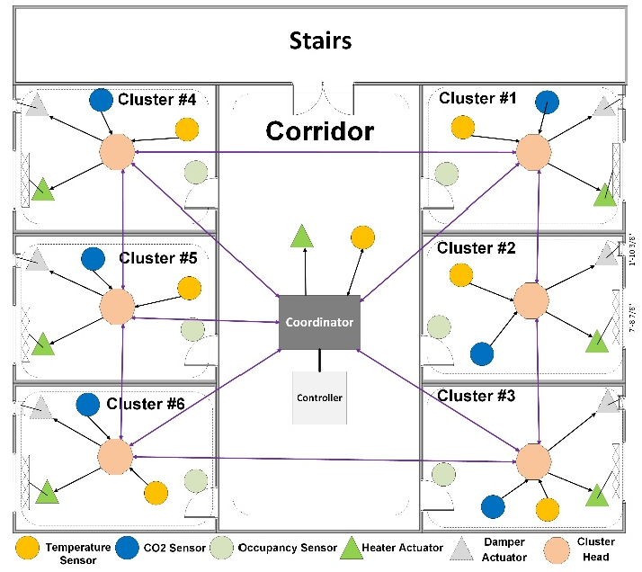
Figure 1 shows an office building scheme [26] for the system model. The system model is implemented based on thermal dependencies among distinct zones. Systems’ inputs and assumptions are according to a typical winter day in February. For each node, the heat transfer differential balance formulas have been modeled [18]. This paper represents a cluster-tree-mesh topology according to the building architecture that supports wireless and battery-powered nodes [22]. Nodes in each cluster send their measured values, to the cluster head and to the controller via the coordinator. Afterwards, the controller processes the received measurements, specifies the commands, and exerts them on the actuators, e.g., heater and damper actuator.
2.1.1. Faults in HVAC Systems
HVAC systems are large-scale systems with numerous components; therefore, faults are unavoidable and must be considered in the design phase. Faults incorporate transient and permanent hardware faults, software faults, and incorrect inputs that can affect the system’s functionality and performance if not satisfactorily handled by fault-tolerance mechanisms.
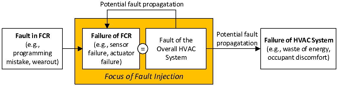
In this paper, we consider each electronic component (i.e., sensor, actuator) as a fault containment region (FCR), which is independent of the immediate impact of a fault in the FCR [27]. The fault injection framework simulates different failure modes of FCRs, thereby allowing the designer to evaluate the resulting behavior of the overall HVAC system. Ideally, the fault-tolerant mechanisms of the HVAC system should ensure that the failure of an FCR (e.g., a sensor) does not propagate to the system boundaries of the HVAC system. If not detected and masked properly, a component-level failure (FCR failure) can cause other FCR failures and, finally, a system-level failure, as illustrated in Figure 2. Using the fault injection framework, the designer can determine the potential fault propagation and the effectiveness of fault-tolerant mechanisms.
Failures of the HVAC system can involve performance degradation, safety risks, surplus cost, and energy waste. From a time perspective, failures of the components may take place during the whole operation of the HVAC system as a permanent fault or as an intermittent fault. Faults with a time dependency can be categorized into abrupt (stepwise/short), incipient, constant, noisy, and intermittent faults [28]. Constant faults arise when a sensor reveals a steady value over time instead of the real and normal sensor readings, and when an actuator sticks to a fixed position. Faults can have an effect on components such as sensors, actuators, computational nodes, and communication networks.
Here, in this paper, the following component faults are applied to our proposed fault injection that are modeled for sensors and actuators values as follow [25]:
- CO2 sensor fault: The CO2 sensor fault resembles an incorrect sensor reading. Five kinds of faults are considered for the sensor components (refer to fault types in Table 2). A gain fault, offset fault, stuck-at value fault, out-of-bound fault, and data loss fault were considered for the CO2 sensor.
- Temperature sensor fault: This type indicates an invalid sensor reading. A gain fault, offset fault, stuck-at value fault, out-of-bound fault, and data loss fault were considered for temperature sensor (refer to fault types in Table 2).
- Damper actuator fault: This type of fault resembles a stuck-at fault when a damper is stuck at a specific position (closed/open). For example, once the damper actuator sticks to the open state (which is equal to the binary value of 1), the open state of the damper actuator causes fresh air to enter into the indoor environment, which decreases the temperature. Therefore, the heater actuator should constantly to compensate for the heat loss (refer to fault types in Table 2).
- Heater actuator (thermostat) fault: This fault describes a stuck-at fault when the heater sticks to a specific position (off/on). For instance, if the heater is stuck at its ON position, it acquires the binary value 1, which means that the indoor temperature rises. If the heater has a stuck-at fault in the OFF position (binary value 0), the temperature tends to decrease (refer to fault types in Table 2).
The equations for each fault type and system faults and their root causes are comprehensively explained in the next section and Table 2.
2.1.2. Faults and Failures Descriptions
In this paper, data-centric faults are modeled, which are related to the generated data from the components [23]. Table 2 shows the fault attributes, including the fault type, fault persistence, fault duration, fault interarrival time, fault repetition, fault location, and faulty value, along with their details and measurement functions. The measurement function calculates the faulty value for each fault type in the faulty states of the system. The following equation describes the generated data for a component of the system that can be modeled as a measurement function over time x’(t) [23]. Equation (1) measures the faulty value to achieve the results of the FI for different fault types:
where:
x represents healthy data;
x’ calculates faulty data;
β is the coefficient of gain faults;
α is the coefficient of offset faults;
η is the coefficient of noise, which is a combination of the Gaussian distribution for measurements and uniform distribution of the measurement uncertainties.
Hardware faults can be classified by their duration into permanent, transient, and intermittent faults:
- Permanent fault: They are caused by a defect in a component that requires the repair or replacement of the component. Examples of permanent faults in HVAC systems are a damper stuck at a closed position or a depleted battery in a sensor.
- Transient fault: Transient faults occur far more often than permanent faults, and they are harder to detect [6]. They are usually caused by environmental conditions such as powerline fluctuations, high-energy particles, and electromagnetic interference.
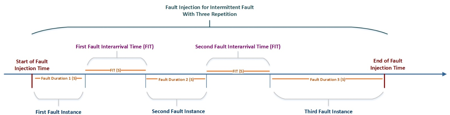
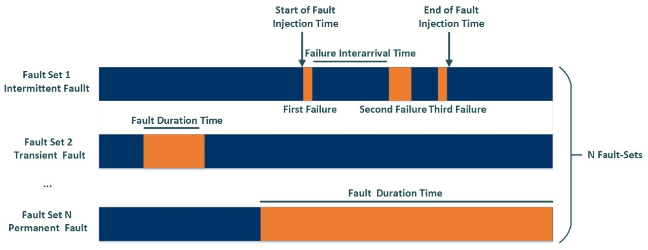
- Intermittent fault: Intermittent faults are temporary malfunctions of a device that are repetitive and occur mostly at irregular time intervals [29]. Intermittent faults have different root causes, such as unstable hardware, varying hardware states, design faults, and wear-out. Intermittent faults can be repaired by replacement or redesign. Most systems incorporate many embedded electronic modules and components to increase the performance of the monitored system. For such complex systems, especially the vehicle industry—trains, ships, and aircraft—intermittent faults become a challenging issue because they increase due to thermal stress, vibration, moisture, and other stresses. In these systems, there are many different reasons for intermittent faults such as loose or corroded wires, cracked solder joints, corroded connector contacst, loose crimp connections, hairline cracks in a printed circuit, broken wires, and unsoldered joints. For example, Wakil et al. discussed intermittent faults and electrical continuity in electrical interconnections [30]. They mentioned some common causes of intermittent faults that can be classified into manufacturing imperfection, connection degradation, interface/coupling, poor design, and intermittent connectivity [30,31]. Examples of intermittent faults in HVAC systems are sensors that are not well-calibrated, software faults, and loose contacts of power or communication lines. In our proposed FI framework, one intermittent fault with two or three repetitions can be modeled. Figure 3 shows the timing diagram of the FI for one intermittent fault with three repetitions. Each fault duration and fault interarrival time was randomly chosen with a uniform distribution.
Table 3 represents the examples of failures in HVAC systems that are mapped to root causes and FCRs. It means that each failure or wrong behavior of the system explains which fault, and in which component, could be the cause. For example, once the system controller detects a high temperature that can have an impact on the system, it must find its root cause, e.g., a stuck-at, gain, offset, or out-of-bound fault. The resource of these faults can be in temperature sensor, heater actuator, or CO2 sensor. For example, when the damper is stuck at a closed status, the level of CO2 increases, and subsequently, the temperature increases.
2.2. Generic Fault Injection Framework in HVAC Systems
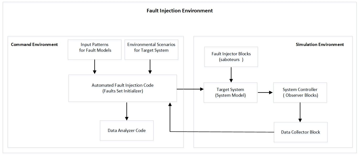
The fault injection environment is depicted in Figure 4, which represents various components of the FI framework in two separate parts of the command and simulation environments. The command environment and simulation environment interact together to activate a fault case example. The environmental attributes and input patterns examine the system and provide data for the fault injection framework and simulated system model. Then, the fault injector blocks initiate the relevant set of attributes for the faults. The fault injector blocks using Stateflow diagrams initialize fault type value and faulty measurements for each input pattern. After the termination of the simulation execution time, the monitoring blocks collect measured data when the test faults are inserted by the fault injector and the test load is succeeded in the system. The output of the simulation is gathered and returned to the fault injection algorithm to be analyzed for fault-tolerant techniques. The modules of the FI environment are listed and explained below.
2.2.1. Command Environment
Input Patterns of Fault Sets
The input patterns of the automated fault injection (AFI) algorithm are shown in Table 4. Each sample can be set by a specific combination of the fault inputs and variables to create fault sets for the system at operation time. A fault location (faulty component) will be selected each time for the fault-initializer algorithm. Other aspects of faults (e.g., timing and persistence) that the system may face during the system operation time are defined in a fault model. In a random fault model, a fault set initiates and affects a particular component in one room. In each fault set, the persistence, types, durations, and interarrival times are initiated. Some samples are illustrated in detail with the fault attributes in Figure 5.
In Figure 5, in the first sample, a fault set with the intermittent persistence type is activated with a sequence of failures with different durations and interarrival times and each failure can have different types and values based on the type of the injected fault. For example, in the case of losing switch contact in measurement devices, an intermittent fault can occur with a sequence of multiple failures. For example, the failure cases can be a sequence of stuck-at, data-loss, or gain faults with three repetitions.
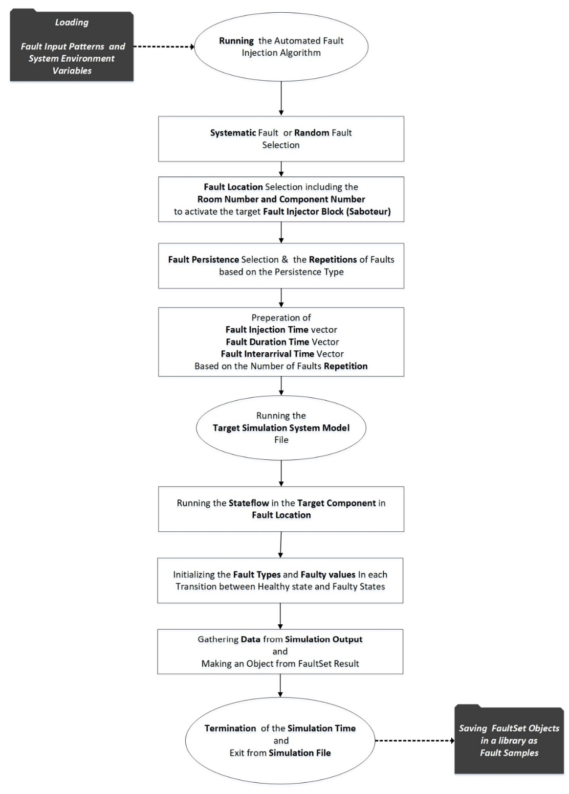
Automated Fault Injection Algorithm
The automated fault injection algorithm (AFIA) loads required variables for the system model and FI process from files as input patterns and environmental scenarios. Two types of faults can be activated in the system: systematic and random faults. In the systematic FI, some components face the same types of faults due to systematic or design problems, e.g., uncalibrated measurement devices from factories, such as sensors, which result in systematic sensor faults. In the random FI, fault attributes can be randomly selected for each fault set. Then, the location of the faults should be clarified to activate a fault set for the target fault-injector blocks (i.e., saboteurs). The room number and component number will show the fault location in the FI process as selected by the algorithm. The persistence type of each fault set should also be determined before running the simulation file. Meanwhile, persistence presents the number of repetitions of the fault injections in each fault set. Then, the simulation runs for each sample time. For example, the execution time can be one day (86,400 s).
In our FI framework, a Stateflow diagram is used to model the persistence feature of the FI framework with different fault duration times and fault interarrival times. In each faulty situation, the state of the system changes between a healthy state and a faulty state for each element of the fault injection vector (e.g., for an intermittent fault with two repetitions, there are two injection times in the fault injection vector). Afterward, in this process, if the fault injection time is equal to the system time, then the state of the system changes. After the corresponding fault duration time, the state of the system returns from the faulty state to the healthy state. Regarding the fault interarrival time (FIT), the state of the system and the signal value is healthy. Fault types and fault values of the system are chosen in each transition of the states, according to the Stateflow model. Figure 6 illustrates the flow diagram with respective steps.
2.2.2. Simulation Environment
Simulation Tools and Model Flow
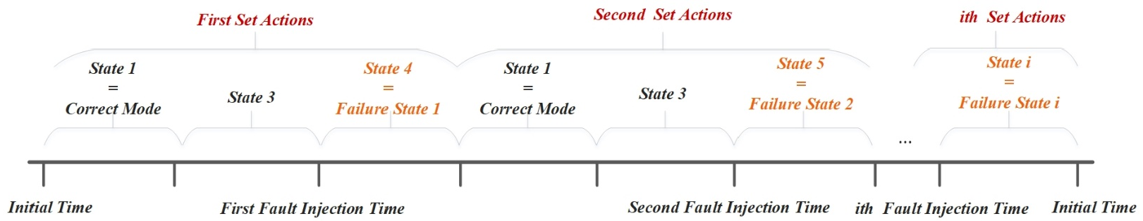
Simulation tools allow a system model to be designed; its parameters can be set and its simulation results can be compared with real world scenarios [23]. To implement the system model, Matlab/Simulink, as a user-friendly tool, is beneficial and is utilized for the implementation of our FI framework. Matlab/Simulink takes advantage of the SimScape blocks to represent a schematic physical system and mathematical equations [23,32]. In addition to modeling the behavior of the system, the finite hierarchical state machine (HSM) is used [33]. Figure 7 represents a timeline for the sequence of the set actions for the FI process. Each set of actions is a sequence of states from the correct mode to failure mode at a related FI time. At the end of each set action, the failure mode returns to the correct mode and then transitions to the second set of actions. This process continues until the last failure mode, and the FI process terminates. For example, for an intermittent fault with three repetitions, three set actions contain three different failure modes.
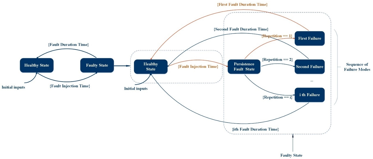
Figure 8 shows a reactive finite-state machine for the FI process between healthy and faulty states. The faulty state consists of the persistence and failure states based on the number of faults (i.e., repetitions). The persistence state determines how many failures occur during the system execution time and the FI process. The model also specifies the transitions to the respective failure state based on the initial inputs, including the FI time and fault duration times that are initialized by the automated fault injection algorithm. For example, in Figure 8, the transitions with different colors define the set actions for the first failure mode, which occurs at the first FI time and first fault duration time. To implement this finite-state machine, a Stateflow diagram is applied to fault injector blocks to produce the faulty values. Each variable of the Stateflow diagram can be a fault attribute, a parameter of the FI process, or a variable of the system model, which can be defined with different types of input, output, local or global parameters. Furthermore, the states change in the state machine during the FI process; Table 5 shows how the states change using the initial input patterns. For example, when the system meets the first fault injection and fault duration time, the state of the system changes to the faulty state, and subsequently, it changes to the healthy and faulty states in the presence of the other fault injection parameters.
Target Simulation System
There are many tools and environments for simulation-based techniques. In this paper, MATLAB/Simulink and MATLAB programming are used for the composition of the simulation code modifications and the simulator command technique. Fault injector blocks including the Stateflow blocks, MATLAB functions and simulation blocks as saboteurs were added to the system model.
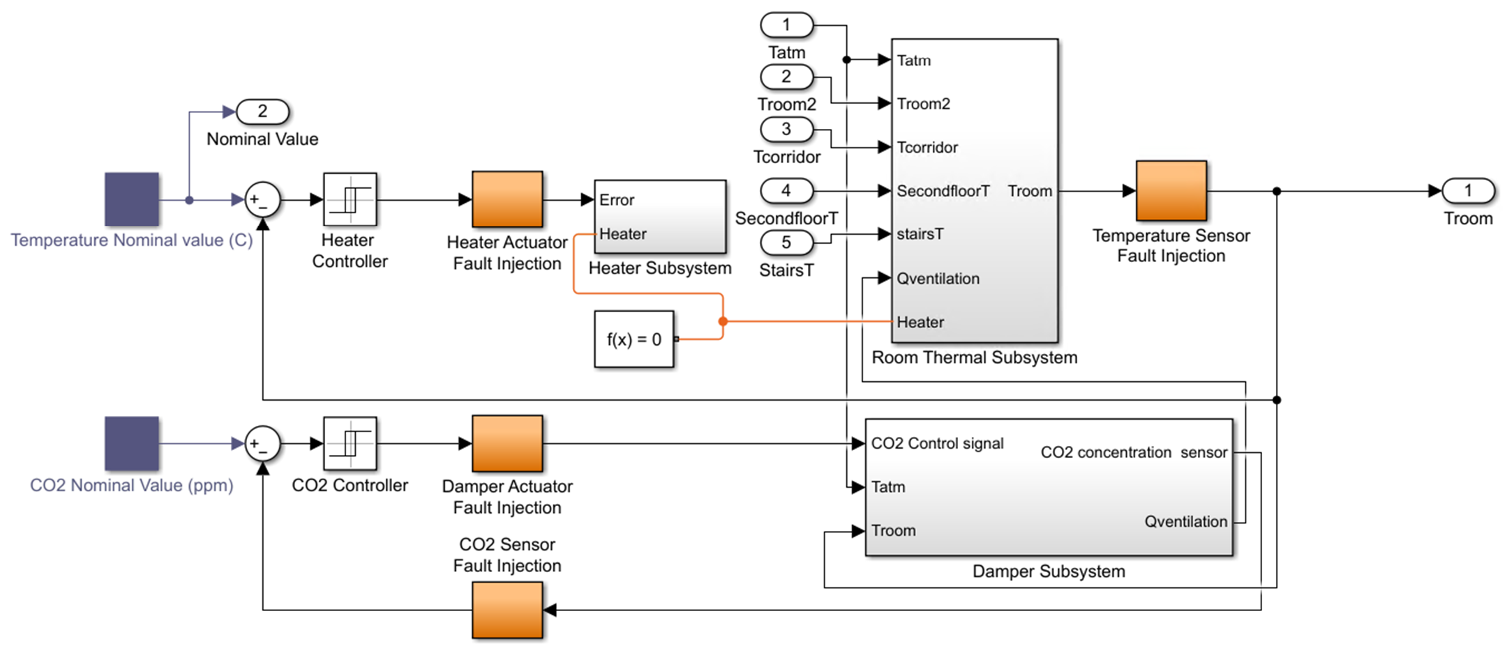
In this framework, there is an automated FI that activates the target saboteur in the system model, which is inactive during its normal operation. For each FI, a fault set (sequence of failures) is injected and for each fault set, some attributes such as fault persistence (i.e., transient, intermittent, permanent), fault location, fault type, fault duration, and fault interarrival time are considered. Moreover, this framework can be evaluated for deterministic fault models (pre-defined fault scenarios) and random fault attributes for single and multiple (systematic) faults at run time. Figure 9 illustrates one zone of an HVAC system, including components and their interconnections, such as the thermal subsystem, damper subsystem, and heater subsystem, which are connected to fault injector blocks. The output of each subsystem is manipulated by the fault injectors (saboteurs).
Fault Injector Blocks (Saboteurs)
A complete overview of the HVAC system‘s components and their interconnections for one room is shown in Figure 9. For each component of the system, one fault injector block is used to manipulate the behavior of the system by changing the measurement value under the specified fault situations. The inner structure of the fault injector block consists of the room number and component number blocks, system measurement data, and system time as input parameters. Finally, the output signal is a merged value of healthy and faulty signals coming from the Stateflow subsystem to ensure an integrated signal. In fault management, the Stateflow diagram controls system reactions. Therefore, we defined the FI framework as a finite-state machine with healthy and faulty states; Figure 8 depicts the situation and transit between healthy and faulty states using the assigned fault attributes. In this paper, a Stateflow diagram is applied as a finite-state machine to control the system’s reactions and their responses under injected faults. The designed state machine in Figure 8 can be mapped to the Stateflow diagram in the Simulink environment. In the interior view of the Stateflow diagram, each FI block is a collection of functions and state diagrams. Fault types and faulty values in each transition of the Stateflow diagram are initialized by calling the related functions. Once the FI process terminates, the data collector blocks gather all information, including faulty and healthy signals, and send them to the automated FI algorithm, then the output of the simulation can be stored in a library.
3. Evaluation, Results and Discussion
The key goal of the proposed fault injection framework is to analyze and monitor system behavior and evaluate the accuracy of the FI framework in diverse fault scenarios. For the evaluation, eight random fault scenarios were studied (Table 6). Hence, for each component, relevant faults were chosen and injected to observe the behavior of the system with its failure impacts, such as occupant discomfort, wasted energy, and risk of fire (refer to Table 3). So, scenarios were chosen according to fault attribute variations and their impacts on the system to show the FI performance. Each example of the scenario was comprehensively explained with fault attributes. Fault parameters were initialized based on the coefficients shown in Table 6, and the faulty signals were measured according to Equation (1). The heater duty cycle and heater energy consumption were set using the designed system model for each scenario, as shown in Table 6. To determine the heating cost, energy consumption was first measured by using the total number of working hours of the heater in one simulation execution (which was considered as one day). The heating cost was considered to be 0.3 EUR/kWh in the system model based on the prices in Germany at the time of writing this paper. The impacts of the CO2 concentration and temperature were also determined, as shown in Table 6, and resembled faulty system-level behaviors. The scenarios are explained one-by-one as follows, and system features and characteristics, such as actual and faulty CO2 concentrations and temperature signals, damper and heater statuses, and heating costs for healthy and faulty situations for each scenario, are depicted.
The occurrence and timing of failures, e.g., failure start times, failure duration times, and failure interarrival times, significantly depended on the application domain. For example, Correcher et al. [34] and Wakil et al. [29] proposed probabilistic strategies to find failure characteristics, such as failure start times, failure duration times, and failure interarrival times, based on experimental data. In Table 6, coefficients for each fault scenario are suggested according to the application domain of this paper, which is a DCV and heating system with sensor and actuator components according to system thresholds, the ranges of variables, and local inputs [23]. Intermittent faults are common in actuators, e.g., damper actuators and thermostats (heater actuators) with relays. The literature suggests certain timing criteria for these kinds of intermittent faults [35,36]. Kuflom et al. investigated the unstable and intermittent faults for numerical and electromechanical overcurrent relays and examined the effect of resetting times on different fault scenarios. They used a pulse generator to generate fault signals and monitor response times [36]. Therefore, in our paper, the timing patterns for intermittent faults of actuators were modeled according to the timing patterns in [35,36].
3.1. Scenario 1
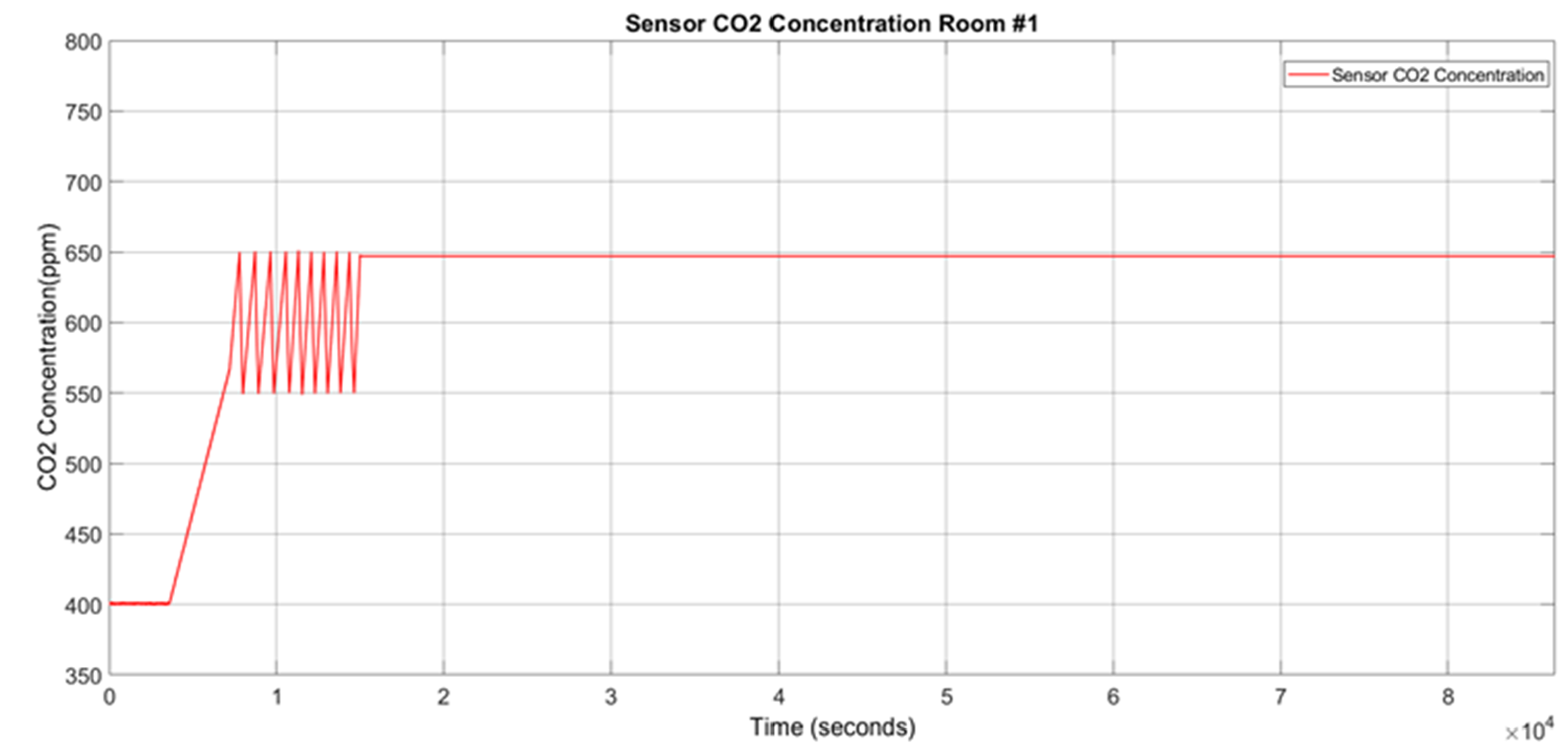
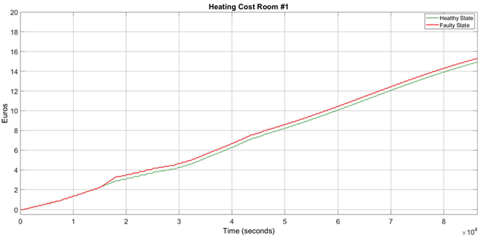
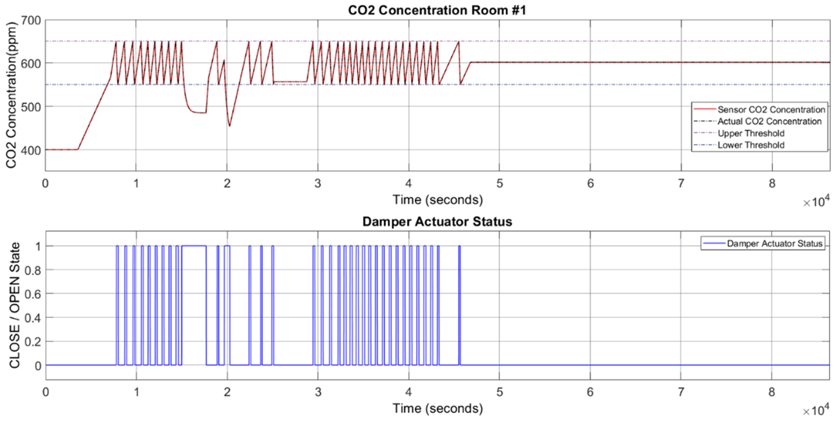
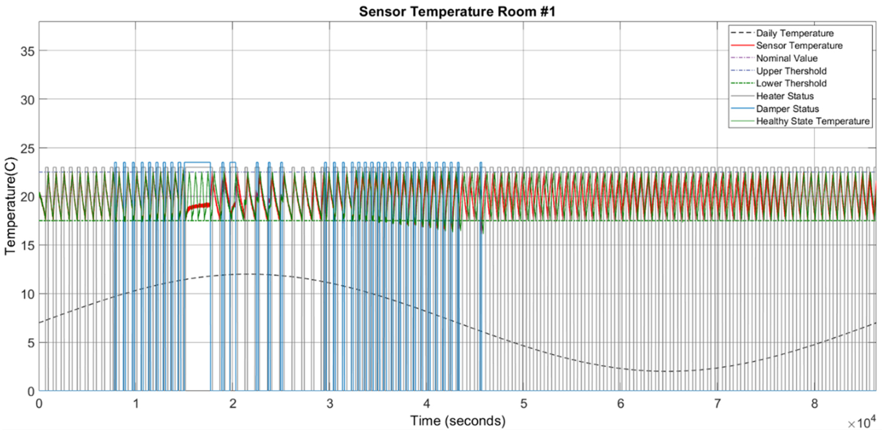
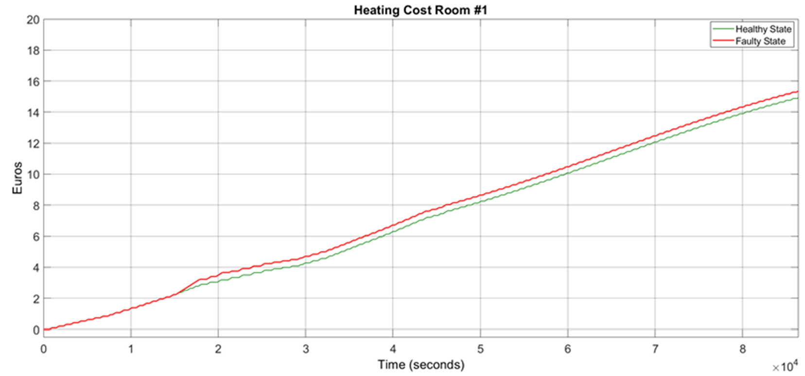
Scenario 1 describes a permanent offset fault for the CO2 sensor and shows the impact of a high CO2 concentration on system behavior, causing a high heater consumption, a clear increase in heating cost, and subsequently, the discomfort of occupants due to lower temperature values. In this scenario, the CO2 sensor has a permanent offset fault with a 125 ppm offset coefficient value. This fault is injected at 15,000 s. In the healthy mode of the system model, whenever the CO2 concentration increases, the damper actuator is opened due to the high number of occupants inside the room or increased CO2 sensor concentration. Figure 10 shows the reaction of the damper subsystem to the offset fault in CO2 sensor which causes an increase in CO2 concentration values from the faulty sensor readings and decrease in real CO2 values due to an opened damper in specific times, respective to the thermal discomfort and temperature decrease, as shown in Figure 11, and energy waste, as shown in Figure 12.
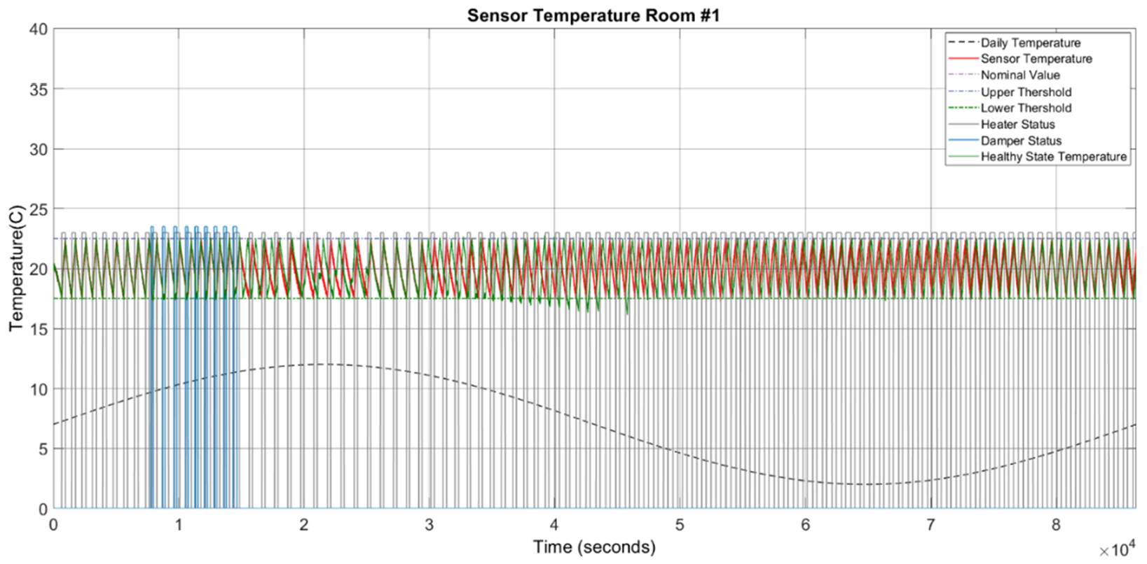
Figure 11 shows the signal variations in the temperature inside the room, which decreases during fault duration because the open status of the damper actuator brings the cold air from the outside to the indoor environment. In the case of permanent faults, the faulty state continues for the rest of the execution time. Since the fault injection increases the concentration value (which is above the upper threshold of 650 ppm), the damper actuator opens, resulting in a decrease in CO2 concentration in the room. Figure 11 shows this temperature drop, which causes occupants’ discomfort.
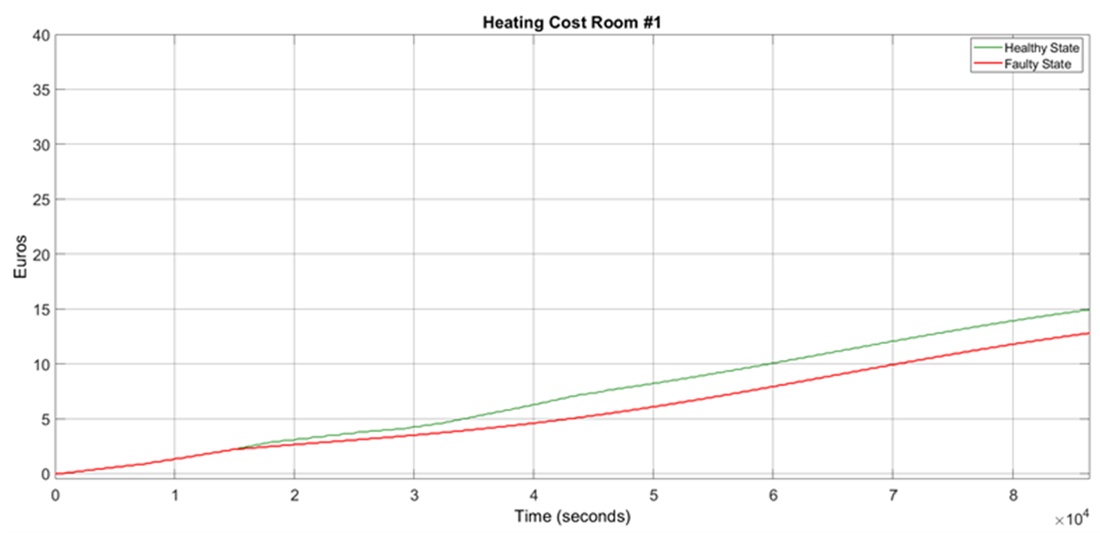
During the whole fault duration, the heater is turned on to compensate the heating load due to the opened damper and to increase the temperature, resulting in an increase in the heater duty cycle, heater energy consumption, and heating costs, as shown in Figure 12.
3.2. Scenario 2
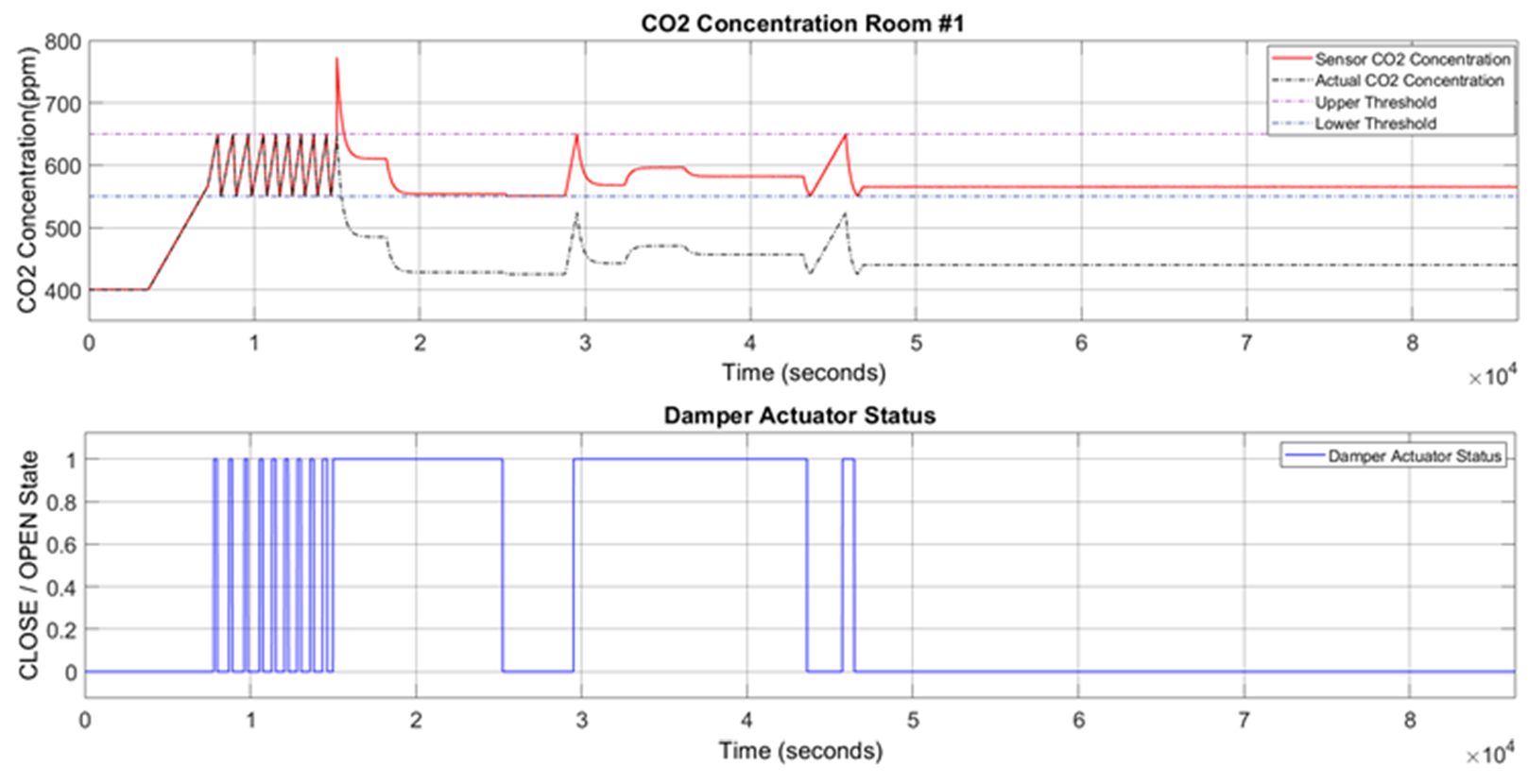
In Scenario 2, the CO2 concentration sensor has a permanent data loss fault. This fault is injected at 15,000 s, which is illustrated in Figure 13. In this scenario, the data loss fault results in the damper actuator becoming stuck at closed, thereby diminishing the load on the heater, which in turn reduces the overall energy consumption compared to a healthy state operation.
Since the CO2 concentration value is within the threshold (650–550 ppm), the damper actuator is closed because the indoor CO2 concentration is in the acceptable range. However, the closed damper actuator status causes an increase in CO2 concentration, as shown in Figure 14. A high amount of CO2 concentration causes the occupants’ loss of concentration, degradation of work efficiency, and other health impacts and even puts their lives in danger.
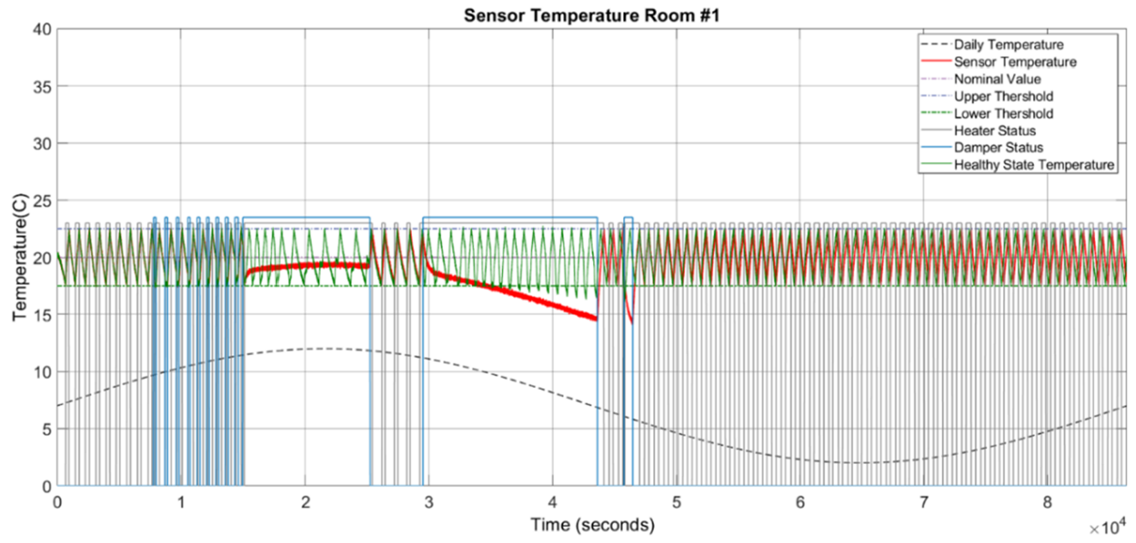
The temperature inside the room stays in an acceptable range during the fault duration because the heater can moderately control the heating load, which is shown in Figure 15.
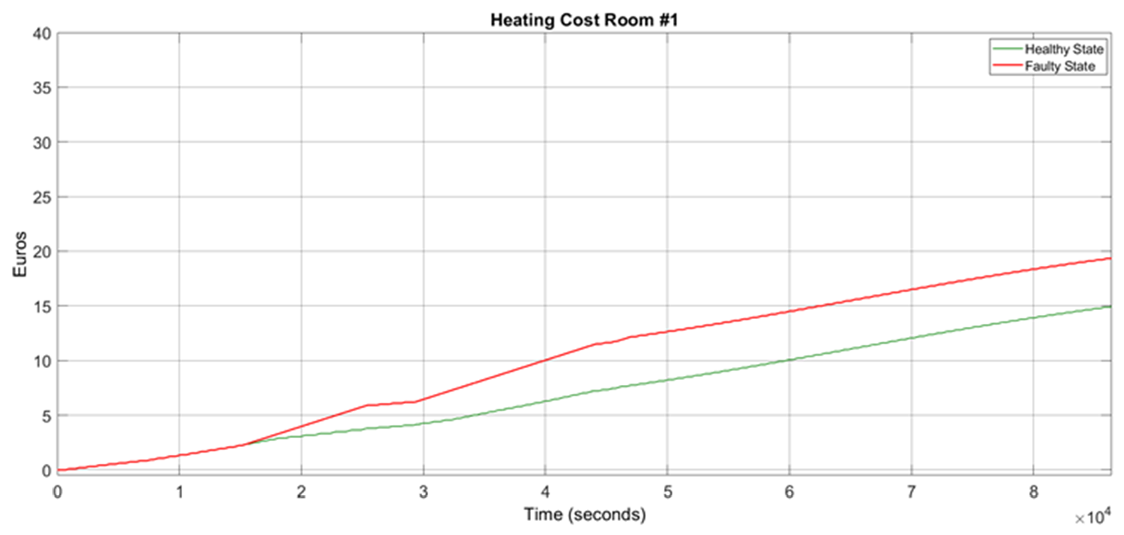
As the damper actuator is closed, no cold air enters the room from the outside environment. This reduces the heating load and causes a lower heater duty cycle and, accordingly, lower heating costs compared to the healthy mode, as illustrated in Figure 16.
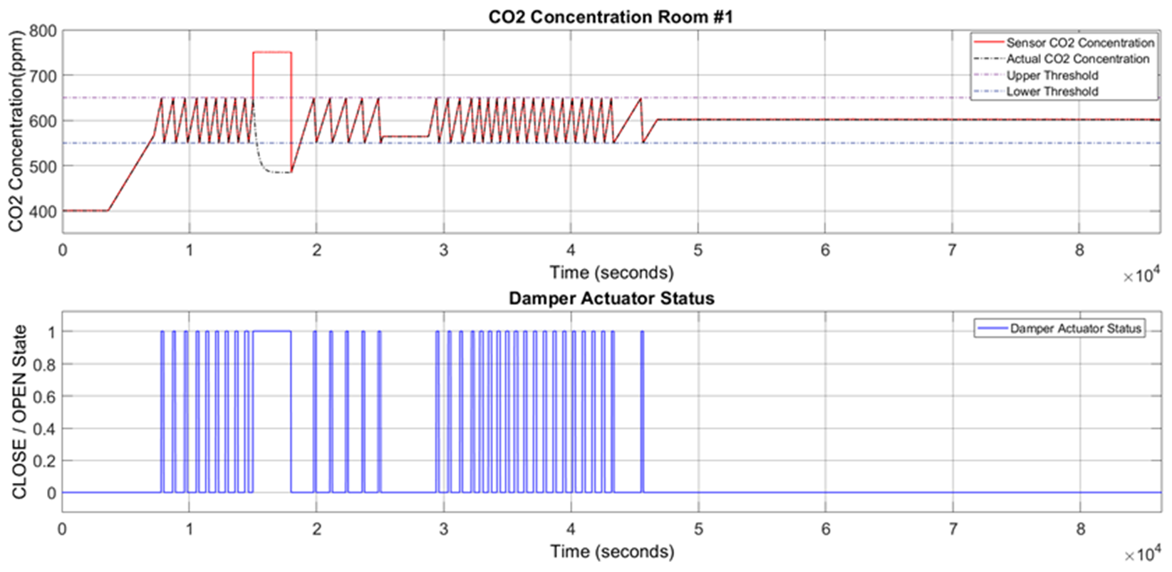
3.3. Scenario 3
Scenario 3 represents a transient stuck-at fault for the CO2 sensor at 750 ppm. This fault is injected at 15,000 s and lasts for the specified fault duration time, which is 3000 s. Since the CO2 sensor concentration is out of the nominal range of 550–650 ppm with a value of greater than 650 ppm, the damper actuator should reduce the CO2 concentration inside the room. So, the damper actuator status changes and opens at 15,000 s, remaining in this situation for a period of 3000 sec, which is clearly shown in Figure 17.
The temperature inside the room decreases during the fault duration as the damper actuator state cause entering the cold air from the environment into the system which is shown in Figure 18. To compensate the heating load due to an opened damper during the fault duration, the heater should remain turned on for a longer time compared to the healthy mode, resulting in an increase in the heater duty cycle and heater energy consumption. Hence, in comparison to the healthy state, there is a slight increase in the heating cost of the system under the faults, as shown in Figure 19.
3.4. Scenario 4
In Scenario 4, an intermittent stuck-at fault with two repetitions is injected into the damper actuator in an open status. The first failure is injected at 15,000 s. This faulty state lasts for 2700 s; thereafter, the damper operation continues in a healthy mode for 2000 sec (interarrival time). Afterward, the second failure is injected into the system, and it lasts for 600 s, then the system operates normally.
Since the damper is stuck at an open state, the CO2 concentration inside the room reduces and reaches the minimum value of 460 ppm. The damper states and changes in the CO2 concentration values can be seen in Figure 20.
The damper status enters the cold air in to the room from the outside environment. This results in a decrease in room temperature, which is depicted in Figure 21. The heater changes to an ON state after 15,000 s to increase the room temperature; however, the temperature will not stay in the acceptable range as the damper actuator, which is illustrated in Figure 21.
The temperature inside the room follows the trend of the environmental temperature during the fault injection time. Therefore, the heater operates at a higher duty cycle and, subsequently, increases the overall energy consumption and heating cost, which is shown in Figure 22.
3.5. Scenario 5
Scenario 5 describes a permanent stuck-at fault for the damper actuator. This fault is injected at 15,000 s. The faulty state endures until the end of the simulation. Since the damper is stuck in an open state, the CO2 concentration inside the room decreases and reaches a minimum value of 400 ppm, which is equal to the outside environment CO2 concentration. The damper’s open status and its strike on the CO2 concentration are depicted in Figure 23.
However, the damper’s open status also decreases the room temperature as shown in Figure 24. The heater changes to an ON state after 15,000 s to increase the room temperature; however, the temperature will not stay in the acceptable range as the damper actuator is open. The indoor temperature follows the trend of the temperature of the outside environment. The heater operates in a high-duty cycle, thereby increasing the overall energy consumption. Consequently, the heating cost considerably increases in comparison with the healthy state operation, as shown in Figure 25.
3.6. Scenario 6
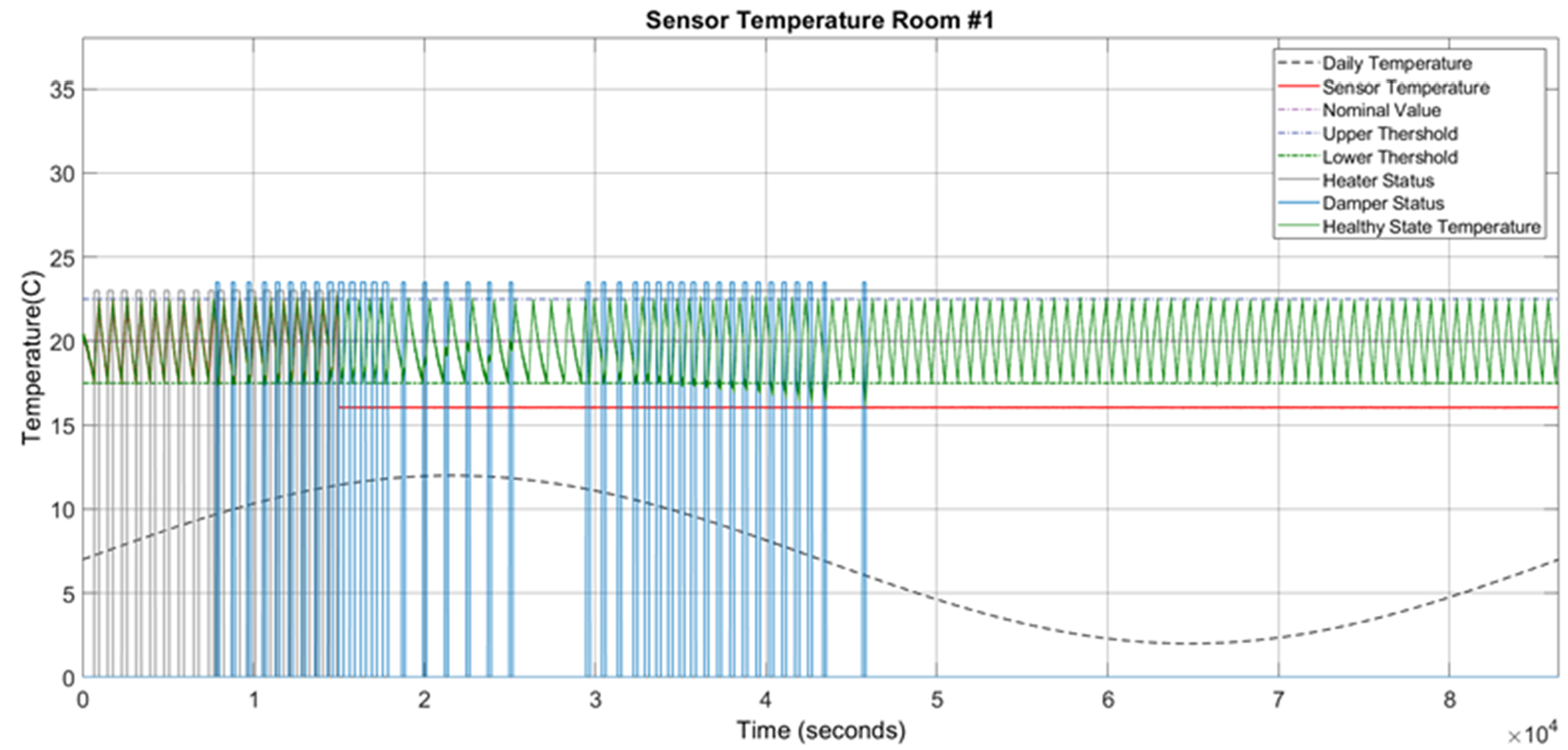
In this scenario, a permanent stuck-at fault is injected into the temperature sensor at 16 °C. This fault is injected at 15,000 s. The faulty state continues for the rest of the execution time until the end of the simulation. The temperature sensor is stuck at a value below the nominal threshold (17.5–22.5 °C), which is depicted in Figure 26.
To increase the inside temperature, the heater should be turned on. However, the damper still functions as intended while the heater is on. Subsequently, the inside temperature of the room increases, as shown in Figure 27.
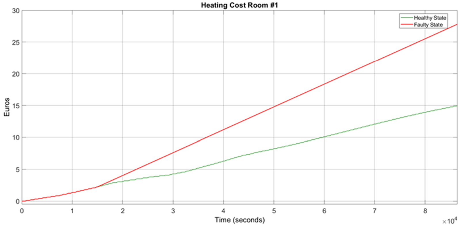
Once the fault is injected, the heater is turned on; therefore, the heater duty cycle and the overall energy consumption increases for the whole fault duration time. Figure 28 shows that the heating cost is considerably increased in comparison with the healthy mode of the system.
3.7. Scenario 7
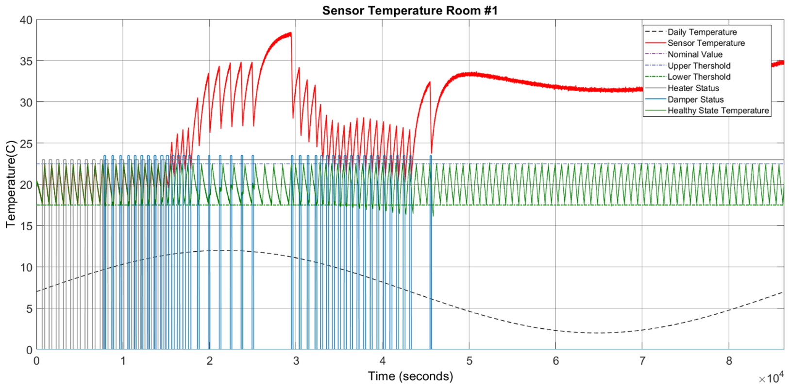
Scenario 7 describes a permanent stuck-at fault for the heater actuator. This fault is injected at 15,000 s and continues until the end of the simulation. When the heater actuator is stuck in the ON state after 15,000 s, the temperature inside the room increases. When the damper status opens, the room temperature decreases, as represented in Figure 29.
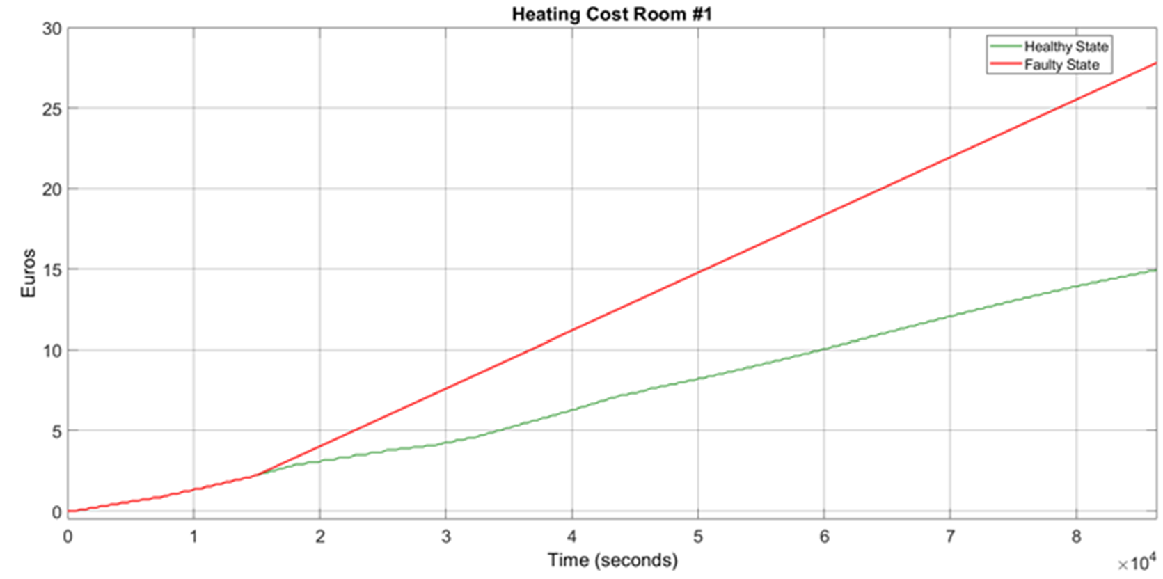
The ON state of the heater results in a higher-duty cycle and increases the energy consumption of the system. Figure 30 shows that the heating cost substantially increases compared to the healthy mode of the system.
4. Conclusions
The evaluation of a system under different faults and anomalies is essential to validate fault-tolerant mechanisms and gain insights into reliability and safety. A simulation-based fault injection provides a high observability and controllability of the deliberate insertion of faults and the monitoring of the system behaviors. One advantage of our proposed automated fault injection framework is that it can be beneficial for different kinds of system models, which must be monitored and evaluated under fault conditions. HVAC systems are an example of such a system, which consists of many sensors and actuators, thereby resulting in a complex and error-prone critical infrastructure. The proposed FI framework was evaluated at the system level based on the component failures of the FCRs. The novelty of the proposed FI framework is that the simulator command technique and simulation code modification were merged for a realistic fault scenario, which can be automatically activated for different fault types with varying attributes. A Gaussian probability and noise with uniform distribution was modeled to reach realistic uncertainties. To implement the fault injectors, a Stateflow diagram was used for the simulation-based fault injection. To evaluate the system model with the new fault injection framework, numerous scenarios were considered. Each of these scenarios allowed us to investigate and understand the behavior of the system under the respective fault case. The evaluation of the framework showed us the consequences of different fault sets, which were activated for specific components, such as sensors and actuators. For each case of the scenarios in the evaluation section, there is a discussion that explains their fault attributes and parameters. Moreover, the figures represent the impact of the fault injection process on the behavior of the system and the signal changes. The faults can also be randomly injected and with random repetitions, which can be useful for evaluating diagnosis techniques. In the example scenarios, we obtained insights into the impact of faults on energy consumption and heating cost. For example, there is a remarkable waste of energy of around +80% in the case of a permanent stuck-at fault in the temperature sensor, which could be avoided using diagnosis and fault tolerance.
Author Contributions
Conceptualization, B.K.; methodology, A.B., B.K. and R.O.; software, A.B. and B.K.; validation, A.B., B.K. and R.O.; formal analysis, B.K. and A.B.; investigation, B.K. and A.B.; resources, B.K., A.B. and R.O.; data curation, B.K. and A.B.; writing—review and editing, B.K., A.B., R.O.; visualization, B.K. and A.B.; supervision, A.B. and R.O.; project administration, A.B. and R.O.; funding acquisition, R.O. All authors have read and agreed to the published version of the manuscript.
Funding
This research including the APC was funded by DFG, grant number OB 384-11-1.
Institutional Review Board Statement
Not applicable.
Informed Consent Statement
Not applicable.
Data Availability Statement
Not applicable.
Conflicts of Interest
The authors declare no conflict of interest.
References
- Sheikh, A.; Kamuni, V.; Patil, A.; Wagh, S.; Singh, N. Cyber Attack and Fault Identification of HVAC System in Building Management Systems. In Proceedings of the in 2019 9th International Conference on Power and Energy System, Peth, WA, USA, 10–12 December 2019; pp. 1–6. [Google Scholar] [CrossRef]
- Choi, K.; Namburu, S.M.; Azam, M.S.; Luo, J.; Pattipati, K.R.; Patterson-Hine, A. Fault diagnosis in HVAC chillers. IEEE Instrum. Meas. Mag. 2005, 8, 24–32. [Google Scholar] [CrossRef]
- Kooli, M.; di Natale, G. A survey on simulation-based fault injection tools for complex systems. In Proceedings of the 2014 9th IEEE International Conference on Design & Technology of Integrated Systems in Nanoscale Era (DTIS), Santorini, Greece, 6–8 May 2014; pp. 1–6. [Google Scholar]
- Song, N.; Qin, J.; Pan, X.; Deng, Y. Fault injection methodology and tools. In Proceedings of the 2011 International Conference on Electronics and Optoelectronics, Dalian, China, 29–31 July 2011. [Google Scholar]
- Lee, D.; Na, J. A Novel Simulation Fault Injection Method for Dependability Analysis. IEEE Des. Test Comput. 2009, 26, 50–61. [Google Scholar] [CrossRef]
- Ziade, H.; Ayoubi, R.A.; Velazco, R. A survey on fault injection techniques. Int. Arab J. Inf. Technol. 2004, 1, 171–186. [Google Scholar]
- Eslami, M.; Ghavami, B.; Raji, M.; Mahani, A. A survey on fault injection methods of digital integrated circuits. Integration 2019, 71, 154–163. [Google Scholar] [CrossRef]
- Jeong, Y.S.; Lee, S.M. A Survey of Fault-Injection Methodologies for Soft Error Rate Modeling in Systems-on-Chips. Bull. Electr. Eng. Inform. 2016, 5, 169–177. [Google Scholar] [CrossRef] [Green Version]
- Lenka, R.K.; Padhi, S.; Nayak, K.M. Fault Injection Techniques-A Brief Review. In Proceedings of the 2018 International Conference on Advances in Computing, Communication Control and Networking (ICACCCN), Uttar Pradesh, India, 12–13 October 2018; pp. 832–837. [Google Scholar]
- Hsueh, M.-C.; Tsai, T.; Iyer, R. Fault injection techniques and tools. Computer 1997, 30, 75–82. [Google Scholar] [CrossRef] [Green Version]
- Maleki, M.; Sangchoolie, B. Simulation-based fault injection in advanced driver assistance systems modelled in sumo. In Proceedings of the 2021 51st Annual IEEE/IFIP International Conference on Dependable Systems and Net-works-Supplemental Volume (DSN-S), Taipei, Taiwan, 21–24 June 2021; pp. 70–71. [Google Scholar]
- Chao, W.; Zhongchuan, F.; Hongsong, C.; Gang, C. FSFI: A full system simulator-based fault injection tool. In Proceedings of the 2011 First International Conference on Instrumentation, Measurement, Computer, Communication and Control, Beijing, China, 21–23 October 2011; pp. 326–329. [Google Scholar]
- Song, L.; Cai, J.; Li, G. Research on simulation-based testability verification method of radar. In Proceedings of the IEEE 2012 Prognostics and System Health Management Conference (PHM-2012 Beijing), Beijing, China, 23–25 May 2012; pp. 1–5. [Google Scholar]
- Gil-Tomas, D.; Gracia-Moran, J.; Baraza-Calvo, J.-C.; Saiz-Adalid, L.-J.; Gil-Vicente, P.-J. Injecting Intermittent Faults for the Dependability Assessment of a Fault-Tolerant Microcomputer System. IEEE Trans. Reliab. 2015, 65, 648–661. [Google Scholar] [CrossRef] [Green Version]
- Evangeline, C.; Sivamangai, N.M. Evaluation of testability of digital circuits by fault injection technique. In Proceedings of the 2015 2nd International Conference on Electronics and Communication Systems (ICECS), Coimbatore, India, 26–27 February 2015; pp. 92–96. [Google Scholar]
- Salih, S.; Olawoyin, R. Fault Injection in Model-Based System Failure Analysis of Highly Automated Vehicles. IEEE Open J. Intell. Transp. Syst. 2021, 2, 417–428. [Google Scholar] [CrossRef]
- Hyvarinen, J. IEA Annex 25 Final Report, Volume I; VTT: Espoo, Finland, 1997. [Google Scholar]
- Behravan, A.; Obermaisser, R.; Nasari, A. Thermal dynamic modeling and simulation of a heating system for a multi-zone office building equipped with demand controlled ventilation using MATLAB/Simulink. In Proceedings of the 2017 International Conference on Circuits, System and Simulation (ICCSS), London, UK, 14–17 July 2017; pp. 103–108. [Google Scholar]
- Wu, S. System-Level Monitoring and Diagnosis of Building HVAC System; University of California: Merced, CA, USA, 2013. [Google Scholar]
- West, S.R.; Guo, Y.; Wang, X.R.; Wall, J. Automated fault detection and diagnosis of HVAC subsystems using statistical machine learning. In Proceedings of the 12th International Conference of the International Building Performance Simulation Association, Sydney, Australia, 14–16 November 2011; pp. 2659–2665. [Google Scholar]
- Behravan, A.; Mallak, A.; Obermaisser, R.; Basavegowda, D.H.; Weber, C.; Fathi, M. Fault injection framework for fault diagnosis based on machine learning in heating and demand-controlled ventilation systems. In Proceedings of the 2017 IEEE 4th International Conference on Knowledge-Based Engineering and Innovation (KBEI), Tehran, Iran, 27 December 2017; pp. 273–279. [Google Scholar] [CrossRef]
- Behravan, A.; Obermaisser, R.; Abboush, M. Fault Injection Framework for Demand-Controlled Ventilation and Heating Systems Based on Wireless Sensor and Actuator Networks. In Proceedings of the 2018 IEEE 9th Annual Information Technology, Electronics and Mobile Communication Conference (IEMCON), Vancouver, BC, Canada, 1–3 November 2018; pp. 525–531. [Google Scholar] [CrossRef]
- Behravan, A. Diagnostic Classifiers Based on Fuzzy Bayesian Belief Networks and Deep Neural Networks for Demand Controlled Ventilation and Heating Systems. Ph. D. Thesis, Universität Siegen, Siegen, Germany, 2022. [Google Scholar]
- Behravan, A.; Tabassam, N.; Al-Najjar, O.; Obermaisser, R. Composability Modeling for the Use Case of Demand-controlled Ventilation and Heating System. In Proceedings of the 2019 6th International Conference on Control, Decision and Information Technologies (CoDIT), Paris, France, 23–26 April 2019. [Google Scholar]
- Behravan, A.; Kiamanesh, B.; Obermaisser, R. Fault Diagnosis of DCV and Heating Systems Based on Causal Relation in Fuzzy Bayesian Belief Networks Using Relation Direction Probabilities. Energies 2021, 14, 6607. [Google Scholar] [CrossRef]
- Behravan, A.; Abboush, M.; Obermaisser, R. Deep Learning Application in Mechatronics Systems’ Fault Diagnosis, a Case Study of the Demand-Controlled Ventilation and Heating System. In Proceedings of the 2019 Advances in Science and Engineering Technology International Conferences (ASET), Dubai, United Arab Emirates, 26 March–10 April 2019; pp. 1–6. [Google Scholar]
- Obermaisser, R.; Peti, P. The Fault Assumptions in Distributed Integrated Architectures; SAE International: Warrendale, PA, USA, 2007. [Google Scholar] [CrossRef] [Green Version]
- Craig, W.C. Zigbee: Wireless Control that Simply Works; Program Manager Wireless Communications; ZMD America, Inc.: Milpitas, CA, USA, 2004. [Google Scholar]
- Syed, W.A.; Khan, S.; Phillips, P.; Perinpanayagam, S. Intermittent Fault Finding Strategies. Procedia CIRP 2013, 11, 74–79. [Google Scholar] [CrossRef] [Green Version]
- Ahmad, W.S.; Perinpanayagam, S.; Jennions, I.; Khan, S. Study on Intermittent Faults and Electrical Continuity. Procedia CIRP 2014, 22, 71–75. [Google Scholar] [CrossRef] [Green Version]
- Kirkland, L.V. When should intermittent failure detection routines be part of the legacy re-host TPS? In Proceedings of the 2011 International Automatic Testing Conference, AUTOTESTCON, Baltimore, MA, USA, 11–15 September 2011; pp. 54–59. [Google Scholar] [CrossRef]
- Abarkan, M.; M’Sirdi, N.K.; Errahimi, F. Analysis and Simulation of the Energy Behavior of a Building Equipped with RESin Simscape. Energy Procedia 2014, 62, 522–531. [Google Scholar] [CrossRef] [Green Version]
- Lee, E.A.; Seshia, S.A. Introduction to Embedded Systems: A Cyber-Physical Systems Approach; MIT Press: Cambridge, MA, USA, 2016. [Google Scholar]
- Correcher, A.; García, E.; Morant, F.; Quiles, E.; Rodríguez, L. Intermittent failure dynamics characterization. IEEE Trans. Reliab. 2012, 61, 649–658. [Google Scholar] [CrossRef]
- Non-Directional Intermittent Ground Fault Protection. Available online: https://www.webgreenstation.com/non-directional-intermittent-ground-fault-protection-siprotec-5-siemens-si5034/ (accessed on 13 January 2022).
- Kuflom, M.; Crossley, P.A.; Liu, N. Impact of Pecking Faults on the Operating Times of Numerical and Electro-Mechanical Over-Current Relays. In Proceedings of the 13th International Conference on Development in Power System Protection 2016 (DPSP), Edinburgh, UK, 7–10 March 2016. [Google Scholar]
Figure 1.
Realistic office building sketch with cluster-based network topology based on building architecture [22,23,25].

Figure 2.
Fault and failure propagation.

Figure 3.
Generic timing diagram for an intermittent fault with three fault repetitions.

Figure 4.
Fault injection environment overview with all implemented modules in both simulation and command environments.
Figure 4.
Fault injection environment overview with all implemented modules in both simulation and command environments.

Figure 5.
Fault sets for N samples.

Figure 6.
Steps of implementation of the automated fault injection process using Stateflow diagram.

Figure 7.
Timeline for set actions in hierarchical state machines showing the sequence of failure modes.
Figure 7.
Timeline for set actions in hierarchical state machines showing the sequence of failure modes.

Figure 8.
Proposed finite-state machine for implemented Stateflow diagram.

Figure 9.
HVAC system model including fault injector blocks (saboteurs).

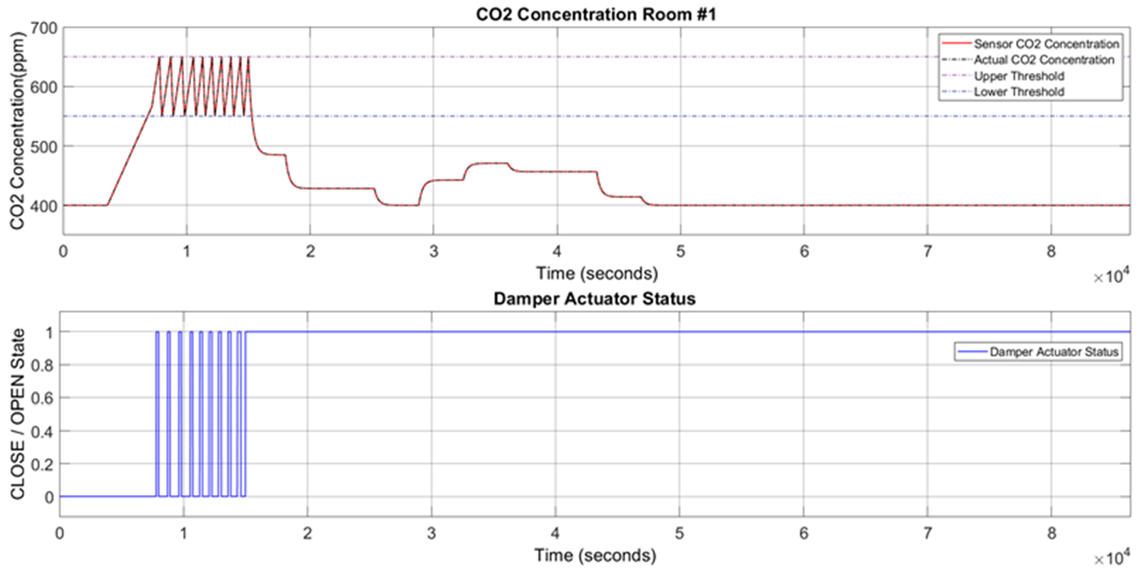
Figure 10.
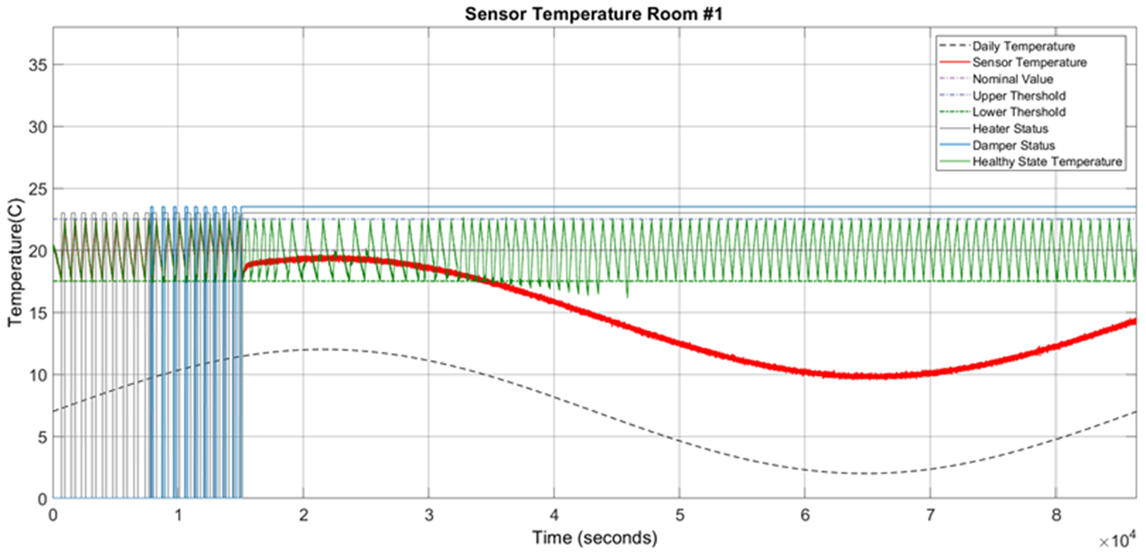
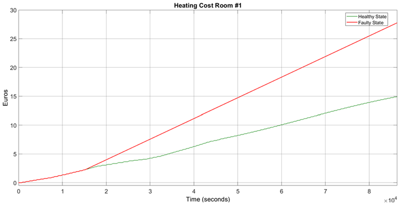
Permanent offset fault of CO2 concentration sensor and damper actuator status (Scenario 1).
Figure 10.
Permanent offset fault of CO2 concentration sensor and damper actuator status (Scenario 1).

Figure 11.
Temperature variation in permanent offset fault of the CO2 concentration sensor (Scenario 1).
Figure 11.
Temperature variation in permanent offset fault of the CO2 concentration sensor (Scenario 1).

Figure 12.
Heating cost measurement for permanent offset fault of the CO2 concentration (Scenario 1).
Figure 12.
Heating cost measurement for permanent offset fault of the CO2 concentration (Scenario 1).

Figure 13.
Zoomed view of faulty CO2 concentration sensor reading in case of permanent data loss fault (Scenario 2).
Figure 13.
Zoomed view of faulty CO2 concentration sensor reading in case of permanent data loss fault (Scenario 2).

Figure 14.
Actual and faulty measurements of a permanent data loss fault for the CO2 concentration sensor vs. damper actuator status (Scenario 2).
Figure 14.
Actual and faulty measurements of a permanent data loss fault for the CO2 concentration sensor vs. damper actuator status (Scenario 2).

Figure 15.
Temperature measurements and variations in CO2 concentration (Scenario 2).

Figure 16.
Heating cost and permanent data loss fault for the CO2 concentration sensor (Scenario 2).
Figure 16.
Heating cost and permanent data loss fault for the CO2 concentration sensor (Scenario 2).

Figure 17.
Actual and faulty measurements for the transient stuck-at fault for CO2 concentration sensor vs. damper actuator states (Scenario 3).
Figure 17.
Actual and faulty measurements for the transient stuck-at fault for CO2 concentration sensor vs. damper actuator states (Scenario 3).

Figure 18.
Temperature variation in the transient stuck-at fault for CO2 concentration sensor (Scenario 3).
Figure 18.
Temperature variation in the transient stuck-at fault for CO2 concentration sensor (Scenario 3).

Figure 19.
Heating cost of the transient stuck-at fault for the CO2 concentration sensor (Scenario 3).
Figure 19.
Heating cost of the transient stuck-at fault for the CO2 concentration sensor (Scenario 3).

Figure 20.
Actual and faulty measurements of the CO2 concentration sensor under an intermittent stuck-at fault for the damper actuator (Scenario 4).
Figure 20.
Actual and faulty measurements of the CO2 concentration sensor under an intermittent stuck-at fault for the damper actuator (Scenario 4).

Figure 21.
Temperature variations in the intermittent stuck-at fault for the damper actuator (Scenario 4).
Figure 21.
Temperature variations in the intermittent stuck-at fault for the damper actuator (Scenario 4).

Figure 22.
Heating cost for the intermittent stuck-at fault in the damper actuator (Scenario 4).

Figure 23.
Actual and faulty measurements for a permanent stuck-at damper actuator fault vs. damper actuator state (Scenario 5).
Figure 23.
Actual and faulty measurements for a permanent stuck-at damper actuator fault vs. damper actuator state (Scenario 5).

Figure 24.
Temperature variations for an intermittent out-of-bound fault with two repetitions in the CO2 concentration sensor (Scenario 5).
Figure 24.
Temperature variations for an intermittent out-of-bound fault with two repetitions in the CO2 concentration sensor (Scenario 5).

Figure 25.
Heating cost for an intermittent out-of-bound fault with two repetitions for the CO2 concentration sensor (Scenario 5).
Figure 25.
Heating cost for an intermittent out-of-bound fault with two repetitions for the CO2 concentration sensor (Scenario 5).

Figure 26.
Actual and faulty measurements for a permanent stuck-at fault at 16 °C for the temperature sensor (Scenario 6).
Figure 26.
Actual and faulty measurements for a permanent stuck-at fault at 16 °C for the temperature sensor (Scenario 6).

Figure 27.
Temperature signal under a permanent stuck-at fault at 16 °C for the temperature sensor (Scenario 6).
Figure 27.
Temperature signal under a permanent stuck-at fault at 16 °C for the temperature sensor (Scenario 6).

Figure 28.
Heating cost for the permanent stuck-at fault at 16 °C for the temperature sensor (Scenario 6).
Figure 28.
Heating cost for the permanent stuck-at fault at 16 °C for the temperature sensor (Scenario 6).

Figure 29.
A permanent stuck-at open-status fault for the heater actuator (Scenario 15).

Figure 30.
Heating cost for a permanent stuck-at open status fault for the heater actuator (Scenario 15).
Figure 30.
Heating cost for a permanent stuck-at open status fault for the heater actuator (Scenario 15).


Table 1.
Overview of simulation-based on fault injection techniques.
| Reference | Fault Profile Characteristics | Simulation Environment | |||
|---|---|---|---|---|---|
| Fault Types | Fault Persistence | Fault Duration | Fault Interveinal Time | ||
| Maleki et al. [11] | Stuck-at value Single bit-flip Double bit flip | Transient Semi-permanent | No | No | SUMO |
| Chao et al. [2] | No | Transient | No | No | SAM |
| Song et al. [13] | Circuit faults | No | No | No | PSPICE and ADS |
| Gil-Tomás et al. [14] | Circuit faults Single or multiple | Intermittent | No | No | VHDL-based fault injection tool (VFIT) |
| Evangeline et al. [15] | Stuck-at bit Stuck-at value Input data word | Transient Permanent 6-bit LFSR | No | Yes | Xilinx software and 4-bit adder and C17 benchmark circuit |
| Behravan et al. [22] | Stuck-at value Stuck-at open/close Stuck-at off/on | Permanent | No | No | MATLAB/Simulink |
| Behravan et al. [21] | Gian fault Off-set fault Stuck-at value Stuck-at open/close Stuck-at off/on | Permanent | No | No | MATLAB/Simulink |
| Behravan et al. [25] | Stuck-at value Stuck-at open/close Stuck-at off/on | Permanent | Yes | No | MATLAB/Simulink and MATLAB/Programming |
| This paper | Gian fault Offset fault stuck-at value Stuck-at open/close Stuck-at off/on Out-of-bound fault Data loss fault | Permanent Transient Intermittent | Yes | Yes | MATLAB/Simulink and Stateflow diagram and MATLAB/Programming |
Table 2.
Fault profile analysis of fault attributes.
| Nr. | Fault Profile | Fault Details | Measurement Functions for Fault Types (Equation (1)) |
|---|---|---|---|
| 1 | Fault type |
stuck-at fault (actuators) | x′ = α+ η (Sensors) and x′ = 0 or 1 (Actuators) |
| x′ = βx + η | ||
| x′ = α + x + η | ||
| x′ > θ1 or x′ < θ2 | ||
| x′ = Last measurement of actual value | ||
| 2 | Fault persistence type |
| |
| 3 | Fault duration time | Uniform distribution of intermittent faults | |
| 4 | Fault interarrival time | Uniform distribution of intermittent faults | |
| 5 | Fault repetition |
| |
| 6 | Fault location (FCRs) |
| |
Table 3.
Fault profile analysis for fault attributes.
| Nr. | Failures | Impact of Failures | Root Cause (Fault) | FCRs |
|---|---|---|---|---|
| 1 | High-temperature value | Occupant discomfort/waste of energy/fire risk/life risk | Stuck-at/gain/offset/high out-of-bound | Temperature sensor, heater actuator, CO2 sensor |
| 2 | Low-temperature value | Occupant discomfort | Stuck-at/gain/offset/low out-of-bound | Temperature sensor, heater actuator, CO2 Sensor |
| 3 | Wrong temperature value | Occupant discomfort/waste of energy/fire risk/life risk | Stuck-at/gain/offset/out-of-bound/data loss | Temperature sensor, heater actuator, CO2 sensor |
| 4 | High carbon dioxide concentration | Occupant discomfort/life risk/fire risk | Stuck-at/gain/offset/high out-of-Bound | CO2 sensor/damper actuator |
| 5 | Low carbon dioxide concentration | Occupant discomfort/waste of energy | Stuck-at/gain/offset/low out-of-bound | CO2 sensor/damper actuator |
| 6 | Wrong carbon dioxide concentration | Occupant discomfort/life risk/fire risk | Stuck-at/gain/offset/out-of-bound | CO2 sensor/damper actuator |
| 7 | Wrong heater actuator signal | Occupant discomfort/waste of energy/fire risk | Stuck-at/stuck-at off | Heater actuator |
| 8 | Wrong damper actuator signal | Occupant discomfort/life risk/waste of energy | Stuck-at/stuck-at close | Damper actuator |
Table 4.
Realistic fault model for a fault set injection.
| Nr. | Properties | Realistic Example for a Fault Set in Automated Fault Injection |
|---|---|---|
| 1 | Number of samples | The number of samples can be randomly defined or manually assigned. Each sample or system execution time is equal to one day or 86,400 s; 30 samples are equal to 30 days (one month) or 60 samples are equal to 60 days (two months). |
| 2 | Model of fault | Random fault happens in one component with different random fault attributes and times. Systematic fault happens in multiple components at the same time and in the same type. |
| 3 | Fault types vector | Fault types are defined as a vector with different IDs: (1: stuck-at, 2: gain, 3: offset, 4: out-of-bound, 5: data loss) |
| 4 | Fault injection time vector | This vector includes the time injections for each FCR failure based on the fault type and its repetitions in one day. In the same way, the first injection time is randomly selected, and others are initialized based on the number of repetitions, fault duration, and fault interarrival times. |
| 5 | Fault injection persistence vector | {Permanent, transient, intermittent} |
| 6 | Repetition vector | {0, 1, 2}; where 0 is for permanent faults, 1 for transient faults, and 2 intermittent faults. |
| 7 | Fault interarrival vector | A vector of minimum fault interarrival time (e.g., 400 s) and maximum fault interarrival time (e.g., 4000 s) that can be selected by the uniform distribution in case of intermittent faults |
| 8 | Fault duration vector | A vector of minimum fault duration (e.g., 300 s) and maximum fault duration (e.g., 3000 s) that can be selected by a uniform distribution in case of transient and intermittent faults |
| 9 | Faulty component (FCR) vector | {1: CO2 sensor, 2: damper actuator, 3: temperature sensor, 4: heater actuator} |
Table 5.
State transition table showing a Stateflow diagram for an intermittent fault with three repetitions.
Table 5.
State transition table showing a Stateflow diagram for an intermittent fault with three repetitions.
| Current State | Healthy State | Faulty State | |||
|---|---|---|---|---|---|
| Inputs | First Failure Mode | Second Failure Mode | Third Failure Mode | ||
| First injection time and duration time | × | ||||
| First interarrival time | × | ||||
| Second injection time and duration time | × | ||||
| Second interarrival time | × | ||||
| Third injection time and duration time | × | ||||
Table 6.
Example fault scenarios for the evaluation of the fault injection framework.
| Fault Set Nr. | Fault Injection Start Time(s) | Component | Fault Persistence | First Fault Duration(s) | Second Fault Duration(s) (In Case of the Intermittent faults) | Fault Interarrival Time (s) | Fault Type | Fault Co-efficient α | Fault Injection Co-efficient β | Heater Duty Cycle (%) | Heater Energy Consumption (KWH) | Energy Consumption Change (in %) | CO2 Concentration Impact | Temperature Impact |
|---|---|---|---|---|---|---|---|---|---|---|---|---|---|---|
| 1 | 150,00 | CO2 sensor | Permanent | - | - | - | Offset fault | 125 ppm | 1 | 62.45 | 64.44 | + 26.67% | √ | √ |
| 2 | 15,000 | CO2 sensor | Permanent | - | - | - | Data loss | Last value | 0 | 41.4 | 42.72 | −13.33 | √ | × |
| 3 | 15,000 | CO2 sensor | Transient | 3000 | - | - | Stuck at | 750 ppm | 0 | 49.51 | 51.1 | +6.25% | √ | × |
| 4 | 15,000 | Damper actuator | Intermittent | 2700 | 600 | 2000 | Stuck at | 1 (on) | 0 | 49.63 | 51.22 | +6.25% | × | × |
| 5 | 15,000 | Damper actuator | Permanent | - | - | - | Stuck at | 1 (on) | 0 | 89.69 | 92.56 | +80% | × | √ |
| 6 | 15,000 | Temperature sensor | Permanent | - | - | - | Stuck at | 16 °C | 0 | 89.83 | 92.71 | +80% | × | √ |
| 7 | 15,000 | Heater actuator | Permanent | - | - | - | Stuck at | 1 (open) | 0 | 47.25 | 48.76 | +80% | × | √ |
Publisher’s Note: MDPI stays neutral with regard to jurisdictional claims in published maps and institutional affiliations. |
© 2022 by the authors. Licensee MDPI, Basel, Switzerland. This article is an open access article distributed under the terms and conditions of the Creative Commons Attribution (CC BY) license (https://creativecommons.org/licenses/by/4.0/).
Share and Cite
MDPI and ACS Style
Kiamanesh, B.; Behravan, A.; Obermaisser, R. Realistic Simulation of Sensor/Actuator Faults for a Dependability Evaluation of Demand-Controlled Ventilation and Heating Systems. Energies 2022, 15, 2878. https://doi.org/10.3390/en15082878
AMA Style
Kiamanesh B, Behravan A, Obermaisser R. Realistic Simulation of Sensor/Actuator Faults for a Dependability Evaluation of Demand-Controlled Ventilation and Heating Systems. Energies. 2022; 15(8):2878. https://doi.org/10.3390/en15082878
Chicago/Turabian StyleKiamanesh, Bahareh, Ali Behravan, and Roman Obermaisser. 2022. "Realistic Simulation of Sensor/Actuator Faults for a Dependability Evaluation of Demand-Controlled Ventilation and Heating Systems" Energies 15, no. 8: 2878. https://doi.org/10.3390/en15082878
Note that from the first issue of 2016, this journal uses article numbers instead of page numbers. See further details here.