Multi-Objective RANS Aerodynamic Optimization of a Hypersonic Intake Ramp at Mach 5

Abstract

The work describes a systematic optimization strategy for designing hypersonic inlet intakes. A Reynolds-averaged Navier-Stokes database is mined using genetic algorithms to develop ideal designs for a priori defined targets. An intake geometry from the literature is adopted as a baseline. Thus, a steady-state numerical assessment is validated and the computational grid is tuned under nominal operating conditions. Following validation tasks, the model is used for multi-objective optimization. The latter aims at minimizing the drag coefficient while boosting the static and total pressure ratios, respectively. The Pareto optimal solutions are analyzed, emphasizing the flow patterns that result in the improvements. Although the approach is applied to a specific setup, the method is entirely general, offering a valuable flowchart for designing super/hypersonic inlets. Notably, because high-quality computational fluid dynamics strategies drive the innovation process, the latter accounts for the complex dynamics of such devices from the early design stages, including shock-wave/boundary-layer interactions and recirculating flow portions in the geometrical shaping.

1. Introduction

In recent years, hypersonic flight has gotten even greater attention from the scientific community. Even though significant breakthroughs have been accomplished, several questions remain unanswered. Inlet intakes, in particular, are among the most critical and challenging to design of the numerous hypersonic components since their mechanics are characterized by a large number of unstable events and unexpected flow phenomena. However, the proper operation of a high-speed vehicle is fundamentally dependent on the appropriate functioning of its intake system. The device, in fact, is the critical component that conveys the flow to the engine core; as a result, it plays a unique role in the vehicle’s stability and manoeuvrability and the overall mission’s safety. Because of this, it is often difficult for such components to be correctly designed, particularly when considering boundary layer ingestions or off-operation circumstances. In most cases, quasi-two-dimensional techniques based on the Shock/Expansion Theory (SET) are used in the early design phases, with the flow assumed to be stationary and viscous effects ignored. These assumptions produce geometrical concepts that are generally incorrect, mainly when off-design and upstart situations are encountered or tested. One problem that affects inlet intakes is the intake unstart, which is often associated with a dynamic instability known as buzz. Since it may be triggered either by the ingestion of the boundary layer (little buzz) or by the ejection of a normal shock from the intake and the subsequent emergence of a massive separation bubble (big buzz), inlet buzz is a multifaceted phenomenon.

In the late 1950s, Ferri et al. [1] and Dailey [2] made the first observations of the phenomenon, which continues to affect numerous intake arrangements in super/hypersonic conditions even today. From these pioneering works, several researchers have shown that full-scale experiments are preferable to numerical models in hypersonic applications because of the complexity of the physics involved. In this path, Trapier et al. [3] suggest that the big buzz is most likely related to acoustics phenomena that exist before the buzz begins. Wagner et al. [4], on the other hand, investigate the upstart dynamics of an inlet/isolator model at Mach 5, discovering a wide variety of oscillatory and non-oscillatory frequencies. According to the findings, non-oscillatory flow is characterized by reduced pressure variations and an oblique shock upstream. Lee and Jeung [5] give a basic explanation of the phenomena, categorizing the buzz across a single ramp into five separate regimes from both an experimental and numerical standpoint. Soltani et al. [6] conducted a thorough experimental campaign on axisymmetric inlets at various supersonic Mach numbers and inlet angles of attack. The research includes a comprehensive shadowgraphs collection for both design and off-conditions. Tan et al. [7] experimentally validate a technique for practically monitoring the inlet status under starting and unstarted scenarios. Later on, Soltani et al. [8] classify many forms of Shock/Boundary-Layer Interactions (SBLI) concerning mixed-compression inlets. Schlieren and shadowgraph flow visualization and unsteady pressure recordings are used to explore SBLI ejection under subcritical and buzz conditions. Later on, the same research group [9] demonstrates that the buzz phenomenon is shocked oscillation ahead of the supersonic air intake when its mass flow rate decreases at off-design conditions.

However, experiments are costly and require a significant investment in terms of time and skill to set up and maintain the testing facilities. Furthermore, the probes and the tunnel boundary conditions used to gather the data often cause experiments to alter the results in strong compressible conditions. On the other hand, numerical approaches have gained popularity in recent years, owing to the increasing availability of computing power and the resulting breakthroughs in Computational Fluid Dynamics (CFD). Receiving a precise response via CFD software is also a fascinating prospect, considering the enormous variety of fluid dynamic phenomena that may occur at any moment and in any location inside a hypersonic domain. Thus, several numerical investigations concerning super/hypersonic inlet intakes have appeared, and numerous further contributions arise in the literature as a consequence of the pioneering work of Newsome [10], who first employed numerical modelling better to understand the near-critical and unsteady flow regimes during inlet buzz. Lu and Jain [11] examined inlet fluid mechanics using a finite volume Reynolds-Averaged Navier-Stokes (RANS) model, demonstrating that the buzz cycle may be attributable to both local flow instabilities and acoustic resonance modes. Trapier et al. [12] described flow instabilities concerning inlet intakes using a Delayed Detached-Eddy Simulation (DDES) model. Hong and Kim [13] used RANS to analyze buzz mechanics under different throttling circumstances. The authors discovered that when the throttling ratio drops, the dominating frequency of pressure perturbation rises, resulting in a more oscillatory perturbation pattern. Later, the same authors [14] used the prior model to investigate the unstable behaviour of super/hypersonic inlet intakes in response to changes in mass flow rate. Abedi et al. [15] undertake in-depth numerical studies to model and capture buzz phenomena in a supersonic mixed compression air inlet. The Unsteady-RANS (URANS) system of equations with k-$\omega$ SST closure is solved through an axisymmetric unsteady numerical simulation. James et al. [16], on the other hand, propose a two-dimensional compressible RANS model in conjunction with wind tunnel experimental data to examine throttling conditions in supersonic inlets by altering the exit area in the form of plug inserts. Yuan et al. [17] numerically analyze the beginning and inlet-engine matching of an axisymmetric variable geometry inlet with complex structure. Finally, De Vanna et al. [18,19] detailed buzz with Large-Eddy Simulation (LES) strategies.

Despite such contributions to hypersonic research, no definitive works have been published that give a thorough categorization and complete design flow charts for improving the performance of a hypersonic intake, beginning with its very early prototype stages. An efficient and robust design, in fact, is often able to make inlet intakes more stable functioning even in upstart or off-operating conditions, increasing the intake envelop and minimizing recirculating region or flow detachments. In this respect, design guided by automatic optimization procedures is now considered the state-of-the-art in many engineering fields, from structural applications [20,21,22], to fluid mechanics and aerodynamic design [23,24], all the way up to the optimization of manufacturing processes or service facilities [25]. In particular, Genetic Algorithms (GA) have become very popular in all the scientific and technical applications where one or more parameters defining a system have to be minimized/maximized. Compared to other non-linear operational research algorithms (e.g., conjugate gradient methods, penalty methods or Monte Carlo strategies), GA are often one of the best options for treating genuinely multi-objective constrained problems since the fitness functions describing the system are treated by combining stochastic and deterministic features operations, broadening the investigation of the research space and elaborating design options even very far from the initial baseline. However, GA suffer from slow convergence to the Pareto front, and hundreds of fitness function evaluations are required to get decent approximations of the optimum surfaces. The problem is particularly felt in fluid mechanics since fitnesses are acquired from CFD calculations, which are highly costly. As a result, after the initial GA implementation by Holland [26], numerous contributions appeared in the literature to accelerate the techniques’ convergence and meet the application needs (see, e.g., [27,28]). In this path, researchers combined GA with non-linear regression algorithms such as Kriging methods, radial basis functions, neural networks, and support vector machines [29,30,31,32], obtaining predictive meta models that allow to drastically reduce the number of iterations to achieve the Pareto front at the expense of errors associated with data interpolation. Nevertheless, despite the intense activity in combining GA with the most disparate engineering applications, very few research activities have focused in employing evolutionary methods to design optimal hypersonic devices, and the majority of such works aimed at optimizing the shock wave train on a pure system and macroscopic level [33], disregarding the difficulties brought by the shock waves’ interaction with the boundary layer. Thus, the blocking effects of severe viscosity events, flow detachments, and recirculations are usually neglected during the early design stages, resulting in time-consuming and non-functional prototypes.

In this scenario, the present research extends and improves early scrutiny of the Authors [34] to specify robust criteria for automatic designing hypersonic inlet intakes. The design approach, which applies to the initial stages of production, is based on the assumption of steady-state viscous flows and employs RANS models in conjunction with GA to generate optimal geometrical solutions to a priori defined goals. The reason why we chose RANS methods to solve the flow field is essentially related to computational costs. It is generally recognized, in fact, that RANS, modelling the whole turbulent spectrum, cannot capture flow unsteadiness and time-varying characteristics such as pressure/velocity fluctuations, being such features very critical for accurately describing SBLI problems [35,36,37,38,39,40,41,42,43,44]. Consequently, lower results accuracy in shock locations, angles, and interaction sites must be accepted for a cheaper computing cost, which is crucial at the early design stages. Scale-resolved methods, in fact, like LES, are hardly integrated with automatic design tools since analyzing hundreds of configurations in a fully wall-resolved LES framework exceeds the standard computational resources available in most scientific computing projects and even more advanced proposals, exploiting highly efficient parallel architectures, hardly affirm sustainability in terms of core/hours for optimization-guided-designs combined with advanced CFD methods. Thus, the proposed approach allows for a good estimation and management of the most complicated features pertained to highly compressible flows, including the deployment of several wavefronts, realistic SBLI predictions, and near-wall fluid mechanics with reasonable computational costs. Furthermore, due to the generality of the proposed methodology, which consists of combining solver data with operational research algorithms to identify the optimal system configurations of a device, the strategy can be easily applied in a vast range of engineering fields, not just to fluid components as presented in this work.

The following is a breakdown of the structure of the current document: Section 2 describes the numerical model in-depth together with the meshing approach. Section 3 explains how the model is tuned and validated using the baseline configuration. Section 4 discusses the geometric parametrization, the optimization approach, and the rationale for choosing the objective functions. Section 5 contains the derived optimum designs’ results and comments. The conclusion and final comments are summarized in Section 6.

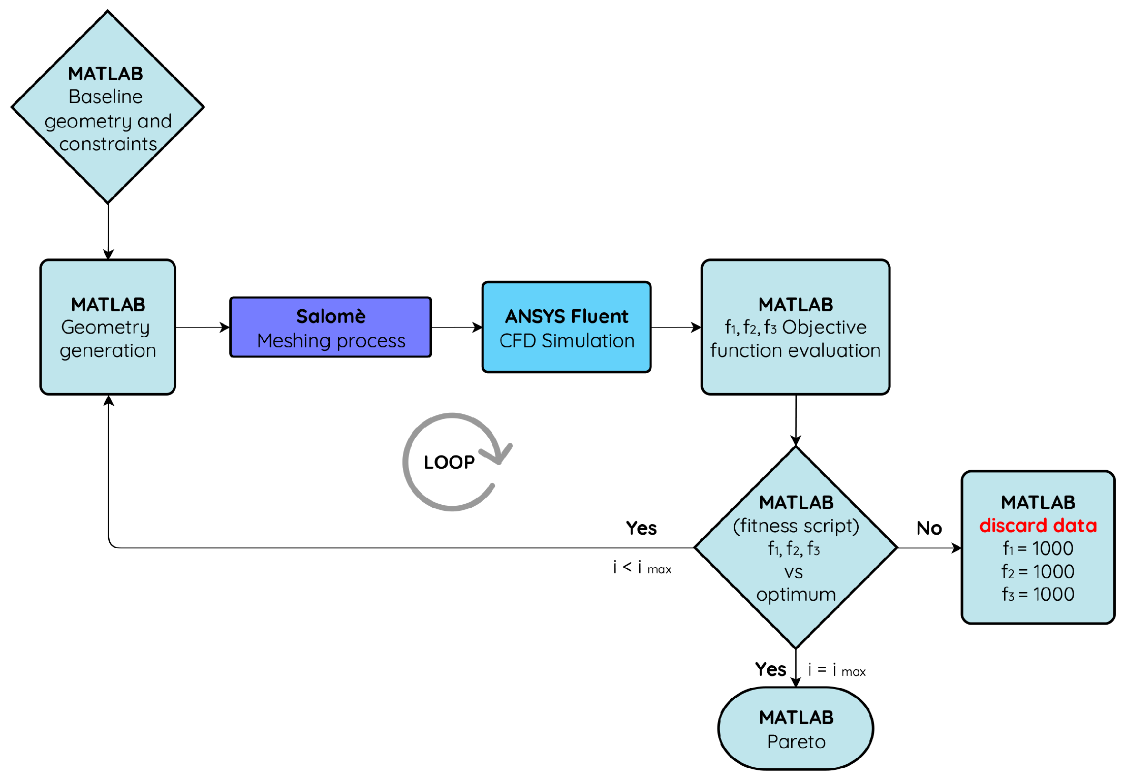
2. Computational Setup and Numerical Methodology

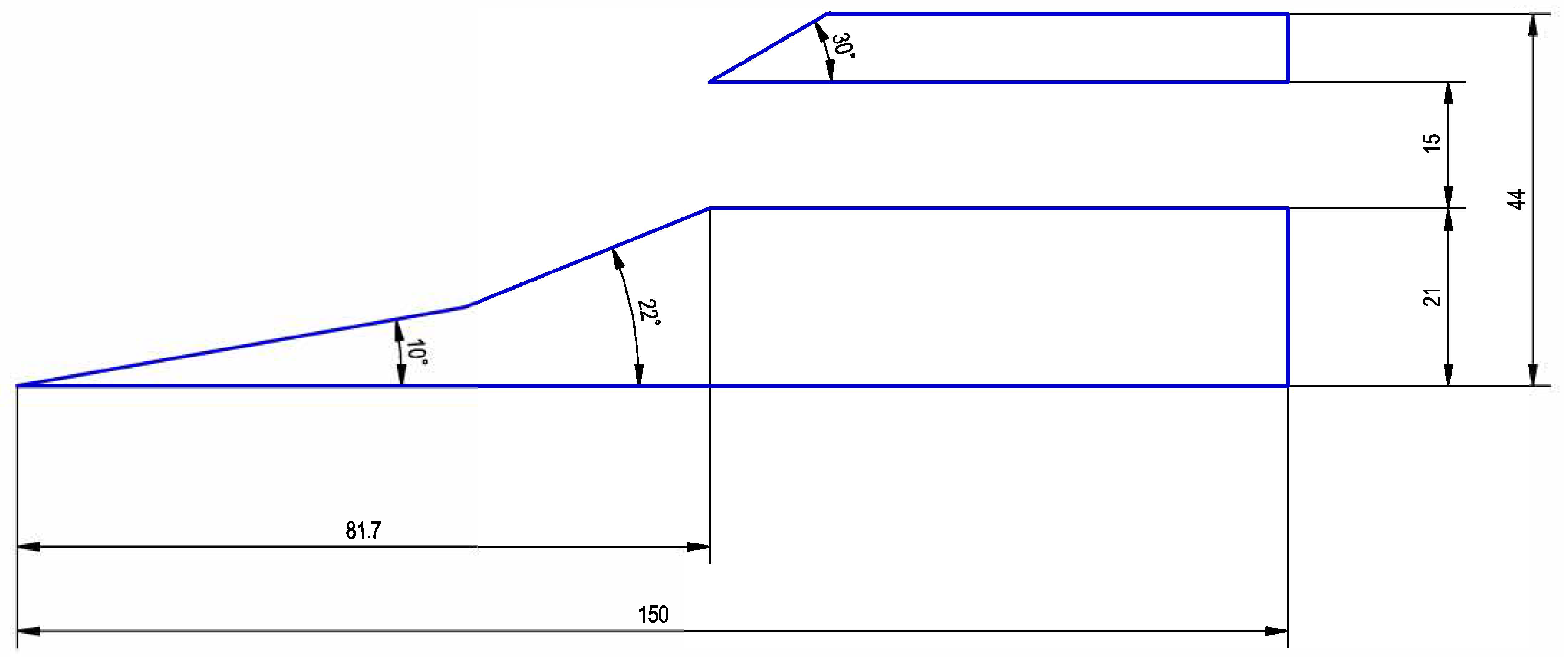
The current work combines commercial and open-source platforms, including Ansys Fluent, Salome (https://www.salome-platform.org), Matlab${}^{\mathrm{TM}}$ (The MathWorks Inc., Matlab, Natick, MA, USA), and Python scripts. Figure 1 reports the intake model’s geometrical properties. The model is precisely equal to that previously analyzed by De Vanna et al. [19]. Unlike [19], the geometry is here reduced to two dimensions, making use of the flow homogeneity and spanwise direction, as customary for RANS models. The intake is divided into two distinct sections: the ramp portion and the cowl lip. The ramp portion, which also corresponds to the intake chord $L_0$, is 150 mm longer and consists of two ramps oriented at ${10}^{\circ }$ and ${22}^{\circ }$ to the horizontal axis, respectively, and an inlet with a height of $2.1$ mm. The cowl lip portion begins vertically at the channel entrance and is defined by a tiny ramp slanted in the streamwise direction by ${30}^{\circ }$. At $0.44$ mm height, a straight roof covers the intake channel. The system dynamics are simulated using a $L_x\times L_y=(1.05\times 0.4)L_0$ mm domain. The fluid domain is subtracted by the intake’s components using boolean operations and divided into six blocks to apply simulation boundary conditions.

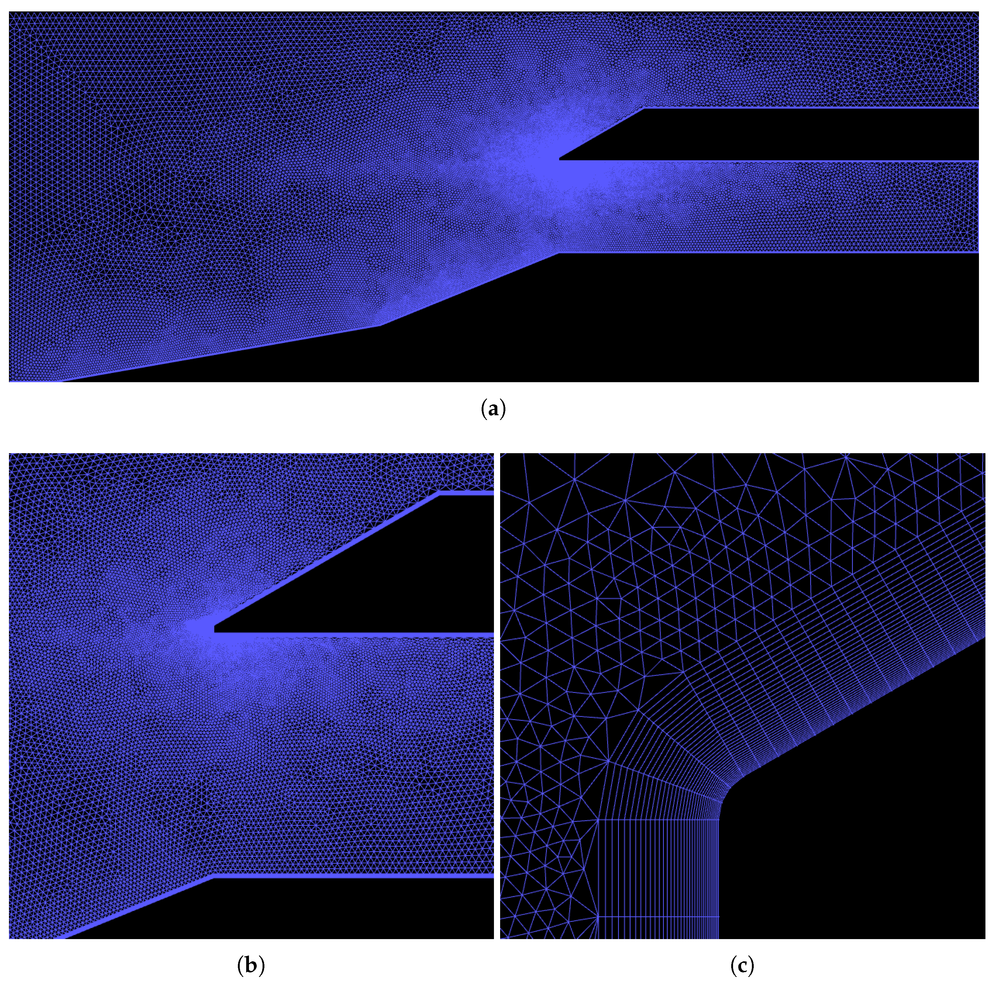
A total of three hybrid and increasingly refined meshes of size roughly 75 k, 150 k, and 300 k elements are used; these are referred to as Coarse (C), Medium (M), and Fine (F). The meshing process is carried out using the open-source Salome platform. Each computational grid is quality tested using the internal software suites, resulting in a mean skewness of $0.22$, a mean inflation growth rate of $1.05$, and a mean orthogonality of 8 for each computational grid. As previously stated, the meshing technique uses a hybrid structured/unstructured approach, with structured cells being employed in the near-wall flow areas. As a result, inflation is set up along the walls in order to improve resolution in the boundary layer and ensure that proper $y_w^{+}=y_w/{\delta }_{\nu }$ values are kept. In particular, we want to address the $y_w^{+}<1$ threshold in order to ensure the quality of boundary layer resolution and to guarantee that the correct resolution is maintained even for trial geometries throughout the optimization process. Here, $y_w$ denotes the first off-the-wall cell distance, while ${\delta }_{\nu }={\mu }_w/\left({\rho }_w{u}_{\tau }\right)$ is the wall local viscous length, ${\rho }_w$ is the wall density, $u_{\tau }=\sqrt{{\tau }_w/{\rho }_w}$ is the friction velocity and ${\tau }_w={\mu }_w\partial u/\partial y$ denotes the wall shear stress. The thermodynamics variables are linked with the ideal gas equation of state, $p/\rho =RT$, where p denotes the thermodynamic pressure, $\rho$ is the fluid density, and T denotes the temperature. $R=\mathcal{R}/\mathcal{M}$ denotes the specific gas constant, with $\mathcal{R}$ = 8.314 JK${}^{-1}$ mol${}^{-1}$ denoting the universal gas constant and $\mathcal{M}$ = 28.965 g mol${}^{-1}$ denotes the air molecular mass. Sutherland’s two coefficients law is used to correlate temperature and laminar viscosity. Figure 2 reports an overview of the mesh as well as some enlargements in the most critical areas (Figure 2b,c).

The system dynamics are simulated in a steady-state framework by solving the compressible RANS system of equations. Three increasingly sophisticated turbulence models are used, with the expected dynamics in terms of flow fields and near-wall performance metrics compared: the one equation Spalart-Allmaras (SA) model by Spalart and Allmaras [45], the two equations k-$\omega$ Shear Stress Transport (SST) model by Menter [46], and the four equations Transition SST (TSST) model by Menter et al. [47]. The spatial components of the Navier-Stokes equations are treated using the 2nd-order Monotonic Upstream-centered Scheme for Conservation Laws (MUSCL) scheme by Van Leer [48], while gradients are reconstructed using the Ansys Fluent standard implementation of the Least Squares Cell-Based technique. A precomputed tolerance of ${10}^{-6}$ is set as a stopping point for the iterative Navier-Stokes residuals dropping. Each analysis requires around 300 iterations to get the convergence.

In terms of boundary conditions, the following are specified: pressure-far-field is enforced on the domain’s left side, where a free-stream Mach number of $M_{\infty }=u_{\infty }/c_{\infty }$ equal to 5 is imposed. Furthermore, the total pressure, $p_{\infty }^{\circ }$, and total temperature, $T_{\infty }^{\circ }$, are set to 820 kPa and 390 K, respectively. Here, $u_{\infty }$ is the free-stream velocity, whereas the undisturbed speed of sound is denoted by $c_{\infty }$. The inflow condition corresponds to a free-stream Reynolds number $R{e}_{L_0}={\rho }_{\infty }{u}_{\infty }{L}_0/{\mu }_{\infty }=2.3\times {10}^6$. Concerning the inflowing turbulence intensity, some considerations are required. In particular, we observed that the system dynamics is widely affected by the freestream flow character. During the previous LES campaign [19], in particular, it has been observed that the big buzz phenomenon mostly disappears when the undisturbed flow is laminar, while even small percentages of freestream desymmetrization induce intense instabilities in the channel intake, promoting the buzz buffeting. However, big buzz phenomena are not and must not be present in nominal operating configurations such as those investigated in the current work, while little buzz events, i.e., high-frequency fluctuations of the frontal shock system caused by SBLI, can appear even in design conditions. Nonetheless, RANS models can not capture little buzz events but require a turbulent intensity level to be specified. Thus, a turbulent intensity of 1.5% is enforced to ensure compatibility between RANS results and experimental tests, the value being the measured freestream turbulence in the wind tunnel. In terms of the domain’s other sides, on the right, a pressure-inlet condition is imposed, while symmetry is used to represent the upper bound. The whole numerical setup reproduces the previous experimental campaign by Berto et al. [49].

Table 1. Models parameters resume and line styles.

Case	Line Style	Marker	Number of Elements	Turbulence Model
Coarse A			75 k	Spalart-Allmaras [45]
Coarse B			75 k	k-$\omega$ SST [46]
Coarse C			75 k	Transition SST [47]
Medium A			150 k	Spalart-Allmaras
Medium B			150 k	k-$\omega$ SST
Medium C			150 k	Transition SST
Fine A			300 k	Spalart-Allmaras
Fine B			300 k	k-$\omega$ SST
Fine C			300 k	Transition SST

resumes the numerical arrangements concerning the various models and provides the line styles to interpret the following of the paper.

3. Model Validation and Baseline Analysis

The previous section’s numerical model is assessed using global and local flow quantities. The study seeks to establish the best grid level and investigate the influence of the turbulence model on system behaviour to select the most appropriate numerical arrangement for the subsequent optimization.

First, we remark the flow field macroscopic configuration by comparing the experimental Schlieren density field and the numerical solution to the baseline setup. Figure 3 reports the experimental instantaneous Schlieren density field (Figure 3a) as obtained during the experimental campaign (see Berto et al. [49] for details) compared to the grey-shaded density field obtained with present RANS computations (Figure 3b). Numerical results refer to the highest resolution mesh and the TSST model. Regardless of the resolution or turbulence model, the whole set of tested configurations accurately depicts the problem’s macroscopic behaviour. Thus, we skip over characterizing flow concerning the various numerical formats since the intake predicted dynamic exhibits similar behaviour regardless of the numerics. We observe high compatibility between the experimental snapshot and the computational results. In particular, the intake provides a system of somewhat intense oblique frontal waves well resolved by the numerical model. These are caused by the two ramps, with slopes of ${10}^{\circ }$ and ${22}^{\circ }$, which divert the flow into the channel and progressively compress it.

A shock wave with a hybrid oblique/normal character may also be noticed on the cowl lip. The interplay of these three frontal waves results in a complicated structure that includes a normal shock, a triple point, and a flow detachment at the cowl lip. Both the numerical and experimental arrangements show such complex shock behaviour. Despite this, the experimental setup reveals that the normal shock at the channel entry is somewhat ahead of the projected location at the RANS level. This is due to the fact that the experimental apparatus embeds sidewalls, the boundary layer of which provides a non-negligible blockage effect, increasing back-pressure and so maintaining the wave system closer to the cowl lip. Despite this minor discrepancy, the RANS model accurately describes the global field. A strong low-density bubble, in fact, is seen on the channel’s bottom surface. This is enclosed between the right-running shock branch from the triple-point and its reflection toward the channel bottom surface. In both the computational and experimental setups, an expanding fan formed by the abrupt geometrical change between the second ramp and the channel bottom surface is ascending the low-density bubble. Instead, the left-running branch from the triple point consists of a slip line that keeps separate the recirculation zone from the flow core. Again, the RANS solution gives considerable insight even in this flow region compared to the experiments. Finally, it is not worthless to mention that the complexity of the shock structures and discontinuities occurring in the system are distinct and well-resolved by the computational grid, indicating that the selected resolution is sufficient to prevent the waves smearing or other adverse effects due to numerical diffusion. Therefore, based on the compatibility between the experimental flow field and that obtained numerically, we have reasonable ground to believe calculation results are highly reliable.

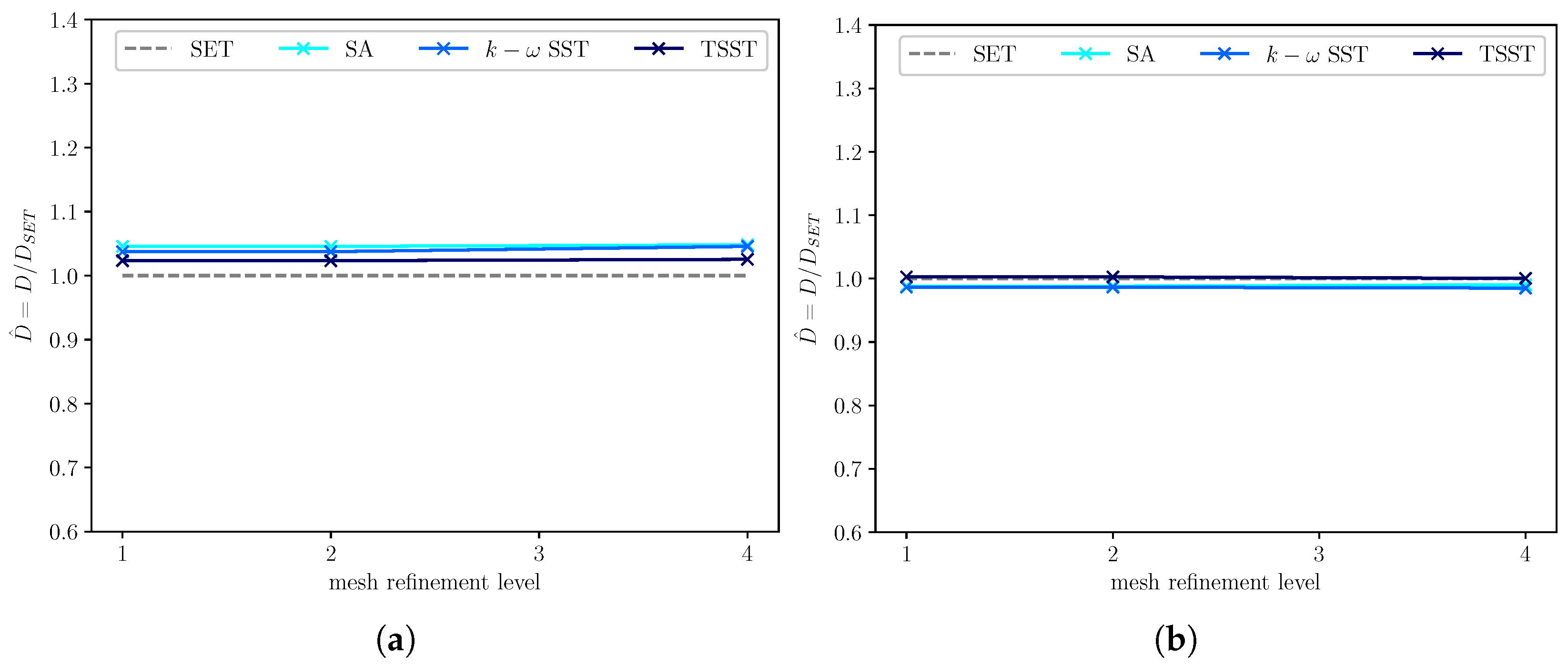
Figure 4 illustrates the ramp SET-scaled drag force, $\widehat{D}=D/D_{SET}$, as a function of the turbulence model and grid refinement. Here, D is the drag force per unit length calculated by integrating the pressure and friction loads over the two ramps, while $D_{SET}$ is the drag force forecast computed using SET formulae. The drag force calculation is confined to ramp surfaces because this area is the only one that can be compared to quasi-two-dimensional predictions based on the SET. According to the rescaling procedure, a $\widehat{D}$ value close to one equals the SET prediction; conversely, the farther the value is from the unit, the larger is the difference between the CFD and SET predictions.

Looking at Figure 4, the compatibility between the two methodologies is very high, even if the CFD data is always somewhat overstated relative to the SET estimation. This behaviour is evident due to SET’s failure to account for viscous terms instead of focusing only on the wall-pressure contribution. However, since shape drag is prominent in the arrangement under evaluation, the consistency between the SET and CFD estimations is extraordinary. The two findings, in fact, differ by no more than 5% independently on the grid level and turbulence model. This indicates that the numerical configurations are resilient and compatible with the physics of the problem at the global level.

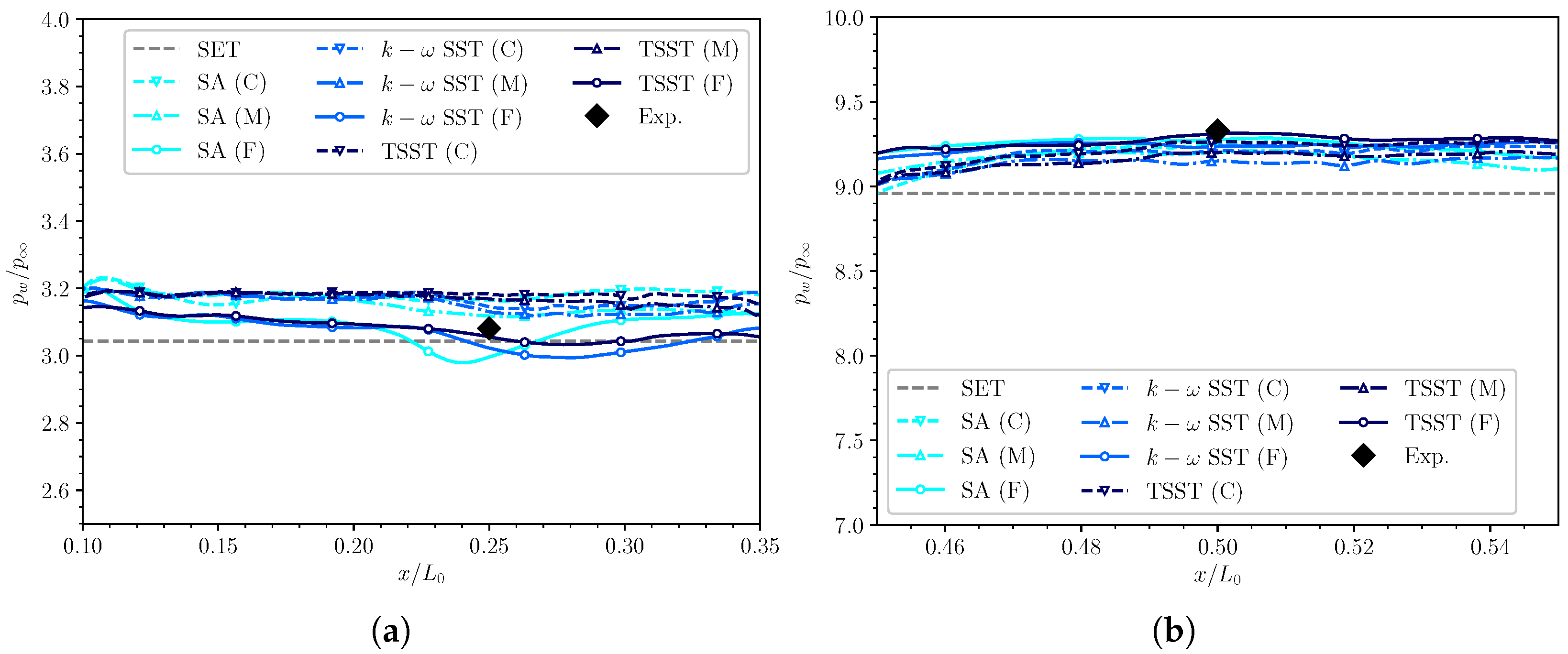
To additionally verify the numerical model, Figure 5 depicts the trend of the freestream scaled wall pressure, $p_w/p_{\infty }$, over the first (Figure 5a) and the second ramp (Figure 5b), respectively. The results, in particular, reflect on the pressure data forecast as a function of grid resolution and parametrically to the turbulence model. Lighter blue tones represent the data acquired with the SA one equation model, whereas deeper blue lines represent the solutions obtained with the k-$\omega$ SST two equations and the TSST four equations models. The grey dashed line still denote the SET wall pressure prediction, whereas the black dot denotes the mean pressure value acquired along the two ramps according to the experiments by Berto et al. [49]. As can be seen, the CFD data are all confined to a relatively tight range and are only moderately affected by the turbulence model used and the refinement level. Furthermore, compliance with the SET data and experimental results assures that the pressure field is appropriately captured by the CFD model, demonstrating the quality of the current numerical model also via local quantities.

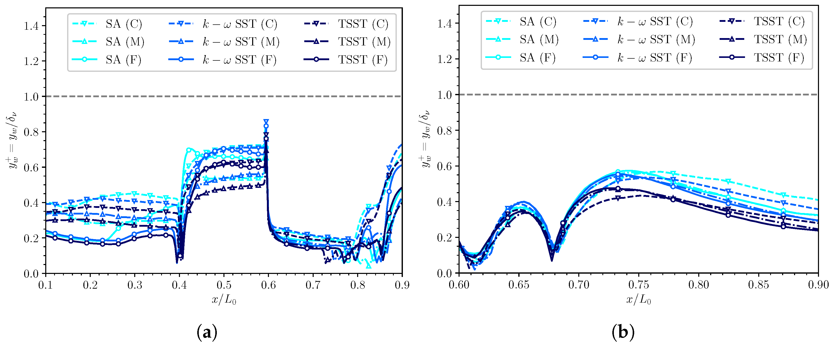
By gradually improving the analysis and being aware that the suggested numerical models are compatible with the physics of the problem, we are now interested in determining whether the proposed computations grids can capture gradients of the fluid quantities adequately. Thus, Figure 6 illustrates the trend of the $y_w^{+}$ wall value, $y_w^{+}=y/{\delta }_{\nu }$, i.e., the inner-scaled distance of the first off-the-wall computational cell. In particular, Figure 6a illustrates the trend relative to the ramp body and the channel’s lower surface, whereas Figure 6b shows the upper wall’s interior surface trend as a function of the chord-scaled streamwise coordinate, $x/L_0$. As the reader can see, all of the chosen meshes provide results close to the suggested threshold for wall-resolved RANS simulations (i.e., $y_w^{+}\simeq 1$), indicating that there are sufficient points inside the boundary layer to capture temperature and velocity gradients near the walls correctly. All grids and the turbulence model, in particular, provide $y_w^{+}$ values considerably below the suggested threshold, resulting in an average $y_w^{+}\simeq 0.5$. Even though such resolution is regarded well resolved concerning wall-turbulence predictions in a RANS framework, we cannot claim a priori that the wall dynamics of the optimization scenarios do not need much higher resolutions than the baseline setup. Thus, since the optimized solutions may result in different wall conditions than the baseline arrangement, such $y_w^{+}$ level give a safety buffer.

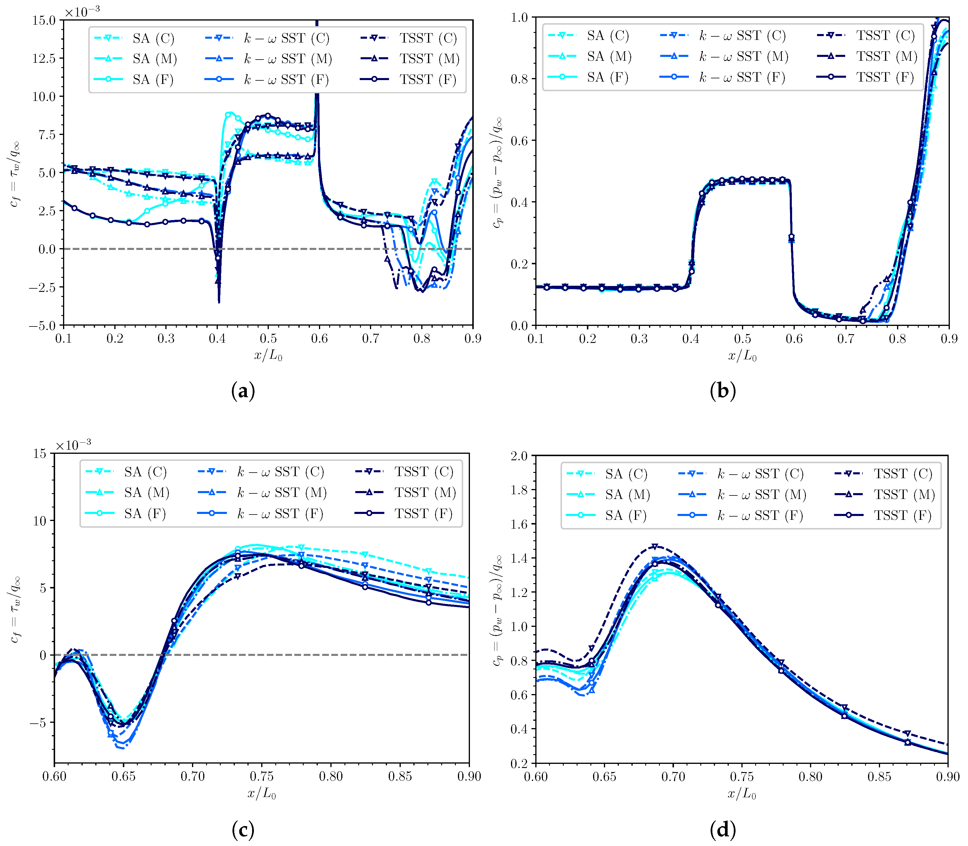
Having understood in quantitative terms that the grid can properly capture the velocity and temperature gradients at the wall, Figure 7 reports the comparison of the results obtained in terms of friction, $c_f={\tau }_w/q_{\infty }$, and pressure $c_p=(p_w-p_{\infty })/q_{\infty }$, coefficients as a function of the grid level and the turbulence model. Here $q_{\infty }=1/2{\rho }_{\infty }{u}_{\infty }^2$ is the freestream pressure load. In particular, Figure 7a,c show the trend of the friction coefficients, while Figure 7b,d show the pressure coefficient along the bottom and the upper channel surfaces, respectively.

Looking at Figure 7a, the findings show that the friction coefficient is reliant on both the grid level and the turbulence model. Even though the friction coefficient values change a bit from model to model and grid to grid, each numerical setup accurately represents the system’s macroscopic behaviour. The flow on the first ramp, in fact, consistently exhibits a flat friction trend caused by a mild transitional boundary layer. Again, all models indicate a significant reduction in wall speed gradient at the ramp junction due to a tiny recirculation bubble. Subsequently, the boundary layer becomes fully turbulent, as seen by the abrupt rise in the friction coefficient at the second ramp. Thus, the sudden geometric transition causes a second velocity wall-gradient discontinuity downstream of the second ramp. All models predict a very consistent pattern with a comparable collapse, the following plateau, and a recirculation zone even in this area. The extension of the latter is highly reliant on the turbulence model and resolution, which is a well-known problem in RANS modelling.

Figure 7c shows the findings in terms of friction coefficient concerning the inner top surface. We see that the flow exhibits an extreme separation in correspondence with the cowl lip, owing mostly to the frontal shock wave, which has a nearly normal nature. The separation causes an extensive recirculation bubble, which rebalances mostly in a $x/L_0=0.1$ space. Compared to the lower surfaces, the friction coefficient trend is significantly more consistent model by model and grid by grid, supporting the accuracy of the various numerical setups again.

Arguing about the pressure coefficient trend along the lower surfaces (Figure 7b) and the inner side of the top surface of the duct (Figure 7d), the wall pressure is very reliable, regardless of the resolution used or the turbulence model. The top internal surface, in particular, has a peak pressure coefficient ranging between $0.675÷0.7x/L_0$ that is accurately headed by all models, practically independently of the grid level. As a result, the pressure coefficient collapses into a relatively narrow range for all the numerical settings, unlike the friction coefficient, which has a more substantial dependence on the turbulence model and the grid.

Gathering the strings of the validation process, the latter reveals that the numerical results are nearly independent of the grid used and the turbulence model employed. As a result, the Fine B model is employed for the following optimization. The model comprises the highest resolved grid-level and the k-$\omega$ SST model. The decision is influenced by the tradeoff of having an efficient numerical arrangement and a flow description almost equivalent to all of the other examined models.

4. Optimisation Procedure

As stated in the introduction, the current work intends to provide an integrated optimization environment suited for the automated design of inlet intakes under super/hypersonic conditions after tuning a suitable numerical model. The stages of the process are as follows. To begin, a baseline intake geometry must be established using experimental criteria or quasi-two-dimensional design techniques. The latter is rebuilt using parametrical approaches, as described in Section 4.1. The baseline geometry is employed as an input for the multi-objective optimization claiming optimal designs concerning a priori defined goals. The definition of the objective functions and the optimization loop is covered in Section 4.2. The geometries, automatically generated by the optimization algorithm, are gradually recombined to the most promising parameters. The assessment of the goal functions using CFD simulations guides the recombination job. As a result, at the conclusion of the process, the algorithm generates a collection of geometrical solutions capable of maximizing/minimizing the design objectives until a certain number of evaluations are completed. Many computational tools are gathered inside the optimization loop through an automated method performed by scripting the individual packages. In particular, the optimization code, written in Matlab, serves as the loop’s driver, creating journal files for Salome and Ansys Fluent throughout loop iterations. A schematic of the whole technique is reported in Figure 8.

4.1. Geometry Parametrisation and Baseline Reconstruction

The parametrization strategy menages the novel shapes by parametrically regulating the geometry aspects (i.e., curves in 2D, surfaces in 3D). At first, the geometric components of the most critical interest must be chosen. In the present study, the ramp portion is selected as the goal of the optimal designing process. This area has the most significant impact on intake performance since the ramp shape determines the whole fluid dynamics in the channel as well as the assessment of the frontal shock system. For the geometrical reconstruction, Bézier splines are adopted. The splines’ parametrization is carried up from the intake leading edge up to the intake channel’s entrance using the following equation:

$$\mathbf{x}\left(t\right)=\sum _{i=0}^n\left(\genfrac{}{}{0pt}{}{i}{n}\right){(1-t)}^{n-i}{t}^i{\mathbf{x}}_i$$

(1)

Here $\mathbf{x}\left(t\right)={\{x\left(t\right),y\left(t\right)\}}^T$ denotes the spline coordinates, ${\left\{\mathbf{x}\right\}}_{i=1}^n={\{x_i,y_i\}}_{i=1}^n$ is the spline control-points set, $t\in$ [0:1] is the curve parameter and n is the spline order. The baseline geometry reconstruction is accomplished out using an in-house developed Matlab program. The algorithm, in particular, takes a baseline geometry and randomly associates a certain number of Bézier splines in the ramp area. The curves are determined by applying a relaxed functional metric logic which holds:

$$\mathcal{I}=\frac{1}{x_1-x_0}{\int }_{x_0}^{x_1}{[{\mathcal{F}}_R\left(\mathbf{x}\right)-{\mathcal{F}}^{*}\left(\mathbf{x}\right)]}^{2}dx$$

(2)

Here $\mathcal{F}{\left(\mathbf{x}\right)}_R$ is a randomly selected spline while $\mathcal{F}{\left(\mathbf{x}\right)}^{*}$ denotes the baseline curve; $x_0$ and $x_1$, with $x_0<x_1$, are the integration extrema. Equation (2) is used as a guideline to determine the initial control point population, ${\left\{{\mathbf{x}}_{0,l}\right\}}_{l=1}^N$, accounting for the distance (in the sense of the function norm) between the randomly selected spline and the baseline geometry. In theory, the technique might be used to find the spline control points, ${\mathbf{x}}_{\mathrm{opt}}$, that best matches the baseline curve by minimizing $\mathcal{I}$. However, such an approach was not pursued since it would lead to confine later optimization to seek solutions around the starting condition. Thus, the optimal reconstructing curve is relaxed concerning randomly generated disturbances. In this work, we employed fifth-order splines, setting $n=5$. Therefore, we use the $N=\mathtt{nInd}=6$ initial individuals. Depending on the number of design goals, the latter are evolved for the $\mathtt{nGen}=40$ and $\mathtt{nGen}=80$ generations for two- and the three-objectives problems, respectively. GA, in fact, suffering from slow convergence to the Pareto front, require hundreds of fitness function evaluations to get decent approximations of the optimum surfaces [26,27,28]. Thus, 240 and 480 trials are tested, respectively, combining the initial N designs up to the convergence of the Pareto front. Such evaluations proved sufficient to populate the Pareto front with satisfactory distributed solutions.

4.2. Definition of the Optimisation Problem and Objective Functions Selection

Once the geometry is parametrized, the current technique aims to determine the optimal geometrical solutions for critical design characteristics. Thus, a multi-objective optimization problem is specified as follows:

$$\left\{\begin{array}{cc}\mathit{minimise}{f}_i\left(\mathbf{x}\right)\hfill & i=1,\cdots ,l\hfill \\ \mathit{subjected}\mathit{to}{g}_j\left(\mathbf{x}\right)\le 0\hfill & j=1,\cdots ,m\hfill \end{array}\right.$$

(3)

here ${\left\{f\right\}}_{i=1}^l$ is the fitness functions set, ${\left\{g\right\}}_{j=1}^m$ denotes the constraints and $\mathbf{x}={\{x_1,\cdots ,x_n\}}^T$ is the decision variables describing the system geometry (i.e., the Bézier control points). The solution of Equation (3) is the Pareto front, which collects the sample of non-dominated designs. In particular, a ${\mathbf{x}}_1$ design is said dominating another ${\mathbf{x}}_2$ if and only if

$$\begin{array}{cc}\hfill \forall i\in [1,l]& f_i\left({\mathbf{x}}_1\right)\le f_i\left({\mathbf{x}}_2\right)\hfill \end{array}$$

(4a)

$$\begin{array}{cc}\hfill \exists j\in [1,l]& f_i\left({\mathbf{x}}_1\right)<f_i\left({\mathbf{x}}_2\right)\hfill \end{array}$$

(4b)

Such a mathematical formulation indicates that no other geometries dominate any Pareto front designs, with the latter gathering the best geometrical compromises. As a result, the Pareto front offers a wealth of information for engineers who practice optimization. The set gathers the best designing solutions in terms of goal functions and constraints, and it provides the best compromise between the various geometries. Thus, within the Pareto front, performance can only be increased at the price of a loss in another.

In the case of a hypersonic intake, the design demands the component to be as little intrusive as feasible in terms of total vehicle drag. Furthermore, the inlet intake must compress the flow, resulting in diffusion and slowing down the stream to the combustion chamber. Finally, systems with oblique compression trains are often selected to avoid energy losses caused by normal shock generation. These ideas are converted into the following three objective functions that must be minimized:

$$f_1=C_d{f}_2=\frac{p_0}{p_1}{f}_3=\frac{p_0^{\circ }}{p_1^{\circ }}$$

(5)

Here $f_1$ is the drag coefficient, $f_2$ is the inverse of the Static Pressure Ratio (SPR) while $f_3$ is the inverse of the Total Pressure Ratio (TPR). In Equation (5) $p_0$ and $p_1$ are the area-weighted static pressures at the intake channel’s entry and exit, respectively, whereas $p_0^{\circ }$ and $p_1^{\circ }$ are the area-weighted total pressures collected at the same places, with $p^{\circ }=p+1/2\rho u^2$. The fitness functions are limited to avoid selecting unphysical designs or flow circumstances. Thus, $f_2$ is restricted to $f_2<1$. All solutions that fall outside this range are flagged with $f_i$ values equal to 1000. The technique does not explicitly constrain operational research but rather penalizes less promising research routes, avoiding selecting unphysical geometrical solutions.

Three distinct optimization campaigns are undertaken to examine the impact of the three goals together and separately. The first includes $f_1$ and $f_2$ goals, which entail searching for solutions with the least drag and the highest SPR. On the other hand, the second campaign provides for the minimization of $f_1$ and $f_3$, intending to find solutions that have the least friction while also the highest TPR. The final set of operational studies is carried out by simultaneously reducing the three goals; thus, seeking solutions with the least drag and the highest static and dynamic pressure ratios.

The multi-objective GA package offered by Matlab is used for optimization. The decision variables are transmitted to a dynamic journal file developed in Python that pivots the Salome meshing algorithm. The Matlab driver script automatically sends the mesh to the Ansys Fluent CFD solver when the mesh is complete. As a result, a new geometrical trial is produced together with a novel set of goals $f_i$. Once the fitness functions are calculated, the GA technique uses their values to generate a new set of geometrical control points, resulting in a new trial design. This new shape is created by combining previously produced geometries and strives to minimize fitnesses. The process results in the Pareto front by iterating up to the maximum number of generations, $\mathtt{nGen}$. The NSGA-II multi-objective genetic algorithm is employed in this work. In particular, the method combines tournament selection, distributed crossover, and Gaussian mutation, with shrink and scale factors set to one. Thus, compared to other optimisation strategies (see, e.g., [31,50]) NSGA-II provides reduced uncertainty in terms of the obtained optimal solutions [32]. The interested reader is addressed to Yijie and Gongzhang [51], Konak et al. [52], Deb et al. [53] for a thorough discussion of the algorithm.

5. Optimization Results

This section displays the results of the optimization approach. To enhance the clarity of the text, the discussion is divided into two subsections. Section 5.1 discusses the bi-objective approach findings, dividing the drag coefficient and the inverse of the SPR minimization ($f_1/f_2$) from the drag coefficient and the inverse of the TPR optimization loop ($f_1/f_3$). Section 5.2 presents the findings of the tri-objective strategy obtained by reducing the drag coefficient while boosting the static and dynamic pressure ratios at the same time $(f_1/f_2/f_3)$.

5.1. Bi-Objective Optimization Results

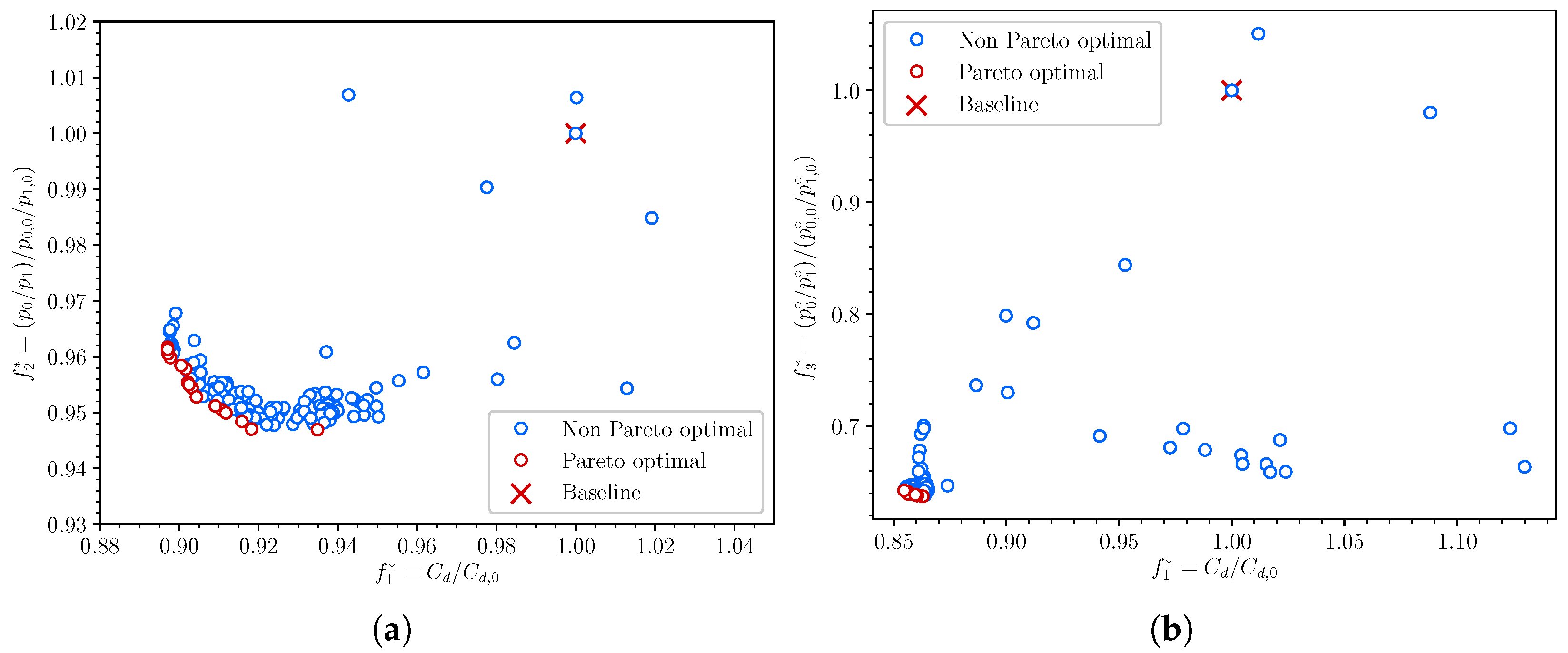
The solutions to the bi-objective optimization problems are shown in Figure 9. In particular, Figure 9a reports the $f_1/f_2$ optimal dataset while and Figure 9b shows the $f_1/f_3$ goals solutions. The plots are made non-dimensional concerning the baseline $f_1$, $f_2$, $f_3$ values so that any point in the plots in the interval $[0:1]\times [0:1]$ represents an improvement compared to the baseline. Blue dots denote the non-optimal findings, while the red dots represent the Pareto optimal collection. In both instances, 240 configurations are evaluated and recombined by merging 6 initial individuals for a number of 40 generations.

5.1.1. $f_1/f_2$ Optimization

Starting with Figure 9a, the Pareto front collects 17 optimal designs and exhibits the typical hyperbolic trend, which is characteristic of a minimum/minimum optimization problem. Nonetheless, the Pareto front is not very extensive, and the extremal instances are different just for a few percentages. In any case, the improvement obtained compared to the baseline case (denoted with a red cross) is significant, offering a reduction of more than 10% for $f_1$ setup and of about 5% for $f_2$. Details are reported in

Table 2. Improvement percentages for the bi-objective optimal designs.

Case	Opt. Loop	$({\mathit{f}}_1-{\mathit{f}}_{1,0})/{\mathit{f}}_{1,0}$	$({\mathit{f}}_2-{\mathit{f}}_{2,0})/{\mathit{f}}_{2,0}$	$({\mathit{f}}_3-{\mathit{f}}_{3,0})/{\mathit{f}}_{3,0}$
Opt. $f_1$	($f_1,f_2$)	−10.3%	−3.87%	-
Opt. $f_2$	($f_1,f_2$)	−6.51%	−5.35%	-
Opt. $f_1$	($f_1,f_3$)	−14.62%	-	−35.8%
Opt. $f_3$	($f_1,f_3$)	−13.68%	-	−36.6%

.

Concerning the $f_1$ and $f_3$ optimization, 7 optimal individuals are gathered in the Pareto set (Figure 9). In this case, the optimal solutions collapse into a single minimal configuration that offers a group of optimal options clustered around a minimum. This should be examined concerning the meaning of the established goals: the drag coefficient and the TPR. Because the TPR highlights the influence of mechanical losses due to turbulent flow areas or regions where the boundary layer recirculates or detaches, the measure indicates comparable performance characteristics to the drag coefficient. Thus, the two pieces of information are not too different, the reason why the Pareto solutions collapse to a single optimal configuration. However, compared to the previous setup, we observe optimizing the drag coefficient together with the TPR produce improved solutions compared to the baseline case, with a $f_1$ reduction of over 10% and a $f_3$ improvement of about 30%. Details are still reported in Table 2.

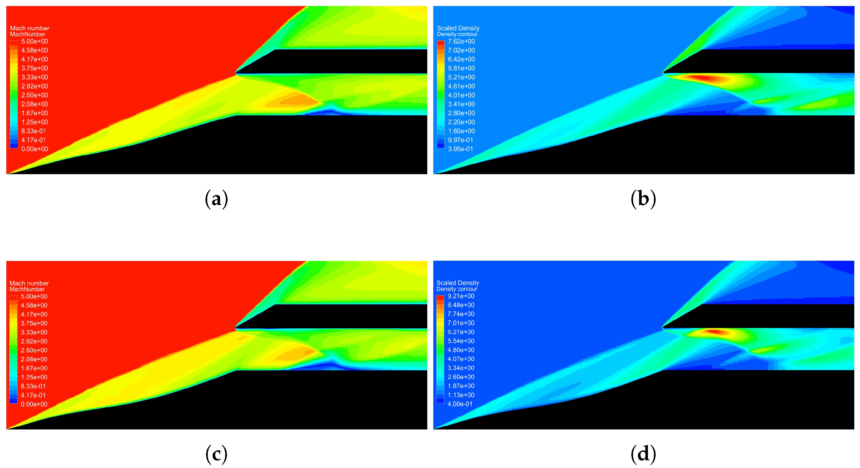
Going through the physical reasons of the gains, we can have a look at the Mach and scaled density fields as reported in Figure 10. The latter collects the two extremal instances corresponding to the $f_1/f_2$ optimization, i.e., the minimal drag design (Figure 10a,b) and the maximum SPR shape (Figure 10c,d). At first glance, the two arrangements do not seem to be much different. The ramps are compressed into a continuous surface that progressively leads the flow from the leading edge to the channel entry. Both solutions show the first ramp with a prominent bulge, causing the oblique wave to shift slope and arrange itself to cross the cowl lip. This shock wave configuration performs very well because it removes the system of the many interactions/reflections that defined the baseline geometry as well as the normal shock wave at the duct entry, resulting in a more stable boundary layer in conjunction with the cowl lip.

However, some substantial differences can be detected between the two optimal designs. The case with minimum drag, in fact, offers an almost linear ramp system, with a very slight curvature between the first and second ramp and a gradual flow compression. This induces a nearly perfect incidence between the oblique wave coming from the leading edge and the upper lip, minimizing the subsequent reflection and considerably reducing the recirculation bubble inside the duct. On the other hand, the setup with the maximum SPR favours the flow rotation between the first and second ramp. The latter shows a decidedly more marked tightening trend with a consequent increase in static pressure according to the intent prescribed by the objective. Therefore, it offers a higher SPR than the previous arrangement but realistically a decidedly narrower envelope due to the difficulty of accommodating flow conditions far from the design for which ramps with marked rotation struggle properly.

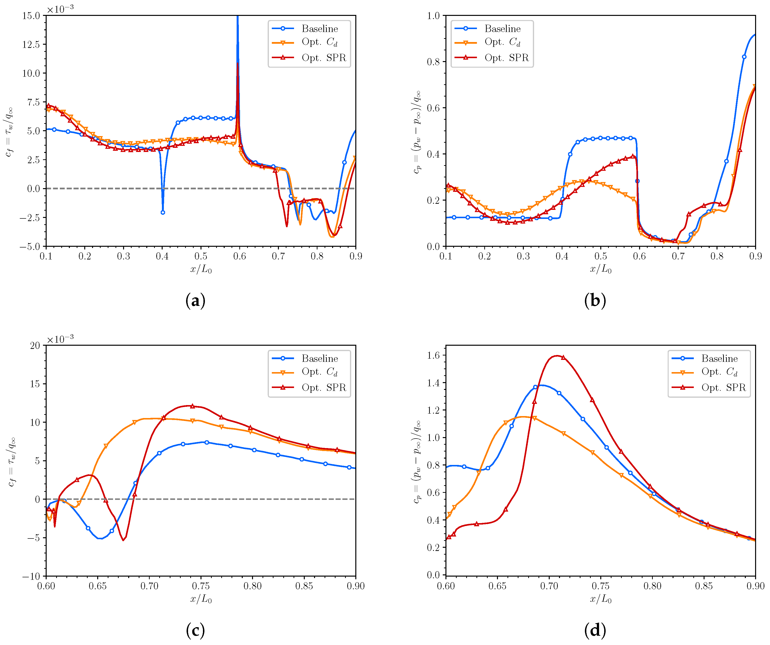
We increase the level of details by comparing the trend of the friction and pressure coefficients for optimal and the baseline solutions, respectively. The results are reported in Figure 11. In particular, Figure 11a,c report the trend of the friction coefficient along the lower and upper surfaces, respectively, while Figure 11b,d report the trend of the pressure coefficient along the same walls.

Figure 11a shows that the friction trend between the ramp body and the bottom surface of the channel is not distinct from the two optimal cases. Thus, a decreasing trend is detected along the first ramp, with a small discontinuity at the duct’s entry. Except for the region associated with the second ramp, where it is significantly decreased, the friction coefficient is similar to the reference case and readjusts to baseline values at the ramp and the channel exit. The recirculation bubble at the exhaust is somewhat more intense for the optimum SPR scenario than in the minimal drag case.

The friction behaviour over the channel’s top surface is much different between the two extremal configurations, as reported in Figure 11c. In particular, the baseline example shows a stagnation zone characterized by a large bubble, while, in both best scenarios, such circumstances are significantly mitigated. In particular, the minimal drag configuration results in an almost disappearing recirculation bubble, condensing it into a small piece at the top lip’s stagnation point. On the other hand, the scenario with maximal SPR allows for a more intense partial detachment and recirculation to the cowl lip, even if it is much more confined than the first attempt solution.

The pressure coefficient’s trend leads to similar conclusions to those reached so far. In Figure 11b, we see a comparison of the baseline pressure coefficient with the least drag and the greatest SPR. When the drag coefficient is kept to a minimum, we maintain a progressive rise in wall pressure up to the duct’s entry. Thus, the pressure level on the ramps is shallow compared to the baseline solution, despite the device’s greater global compression.

Finally, the baseline scenario is halfway between the two optimized cases in terms of the pressure coefficient trend over the top surface (Figure 11d). Indeed, the pressure peak is advanced in the minimal drag design and slightly delayed for the maximal SPR. This is due to the location of the frontal shock wave’s interaction with the top lip.

5.1.2. $f_1/f_3$ Optimization

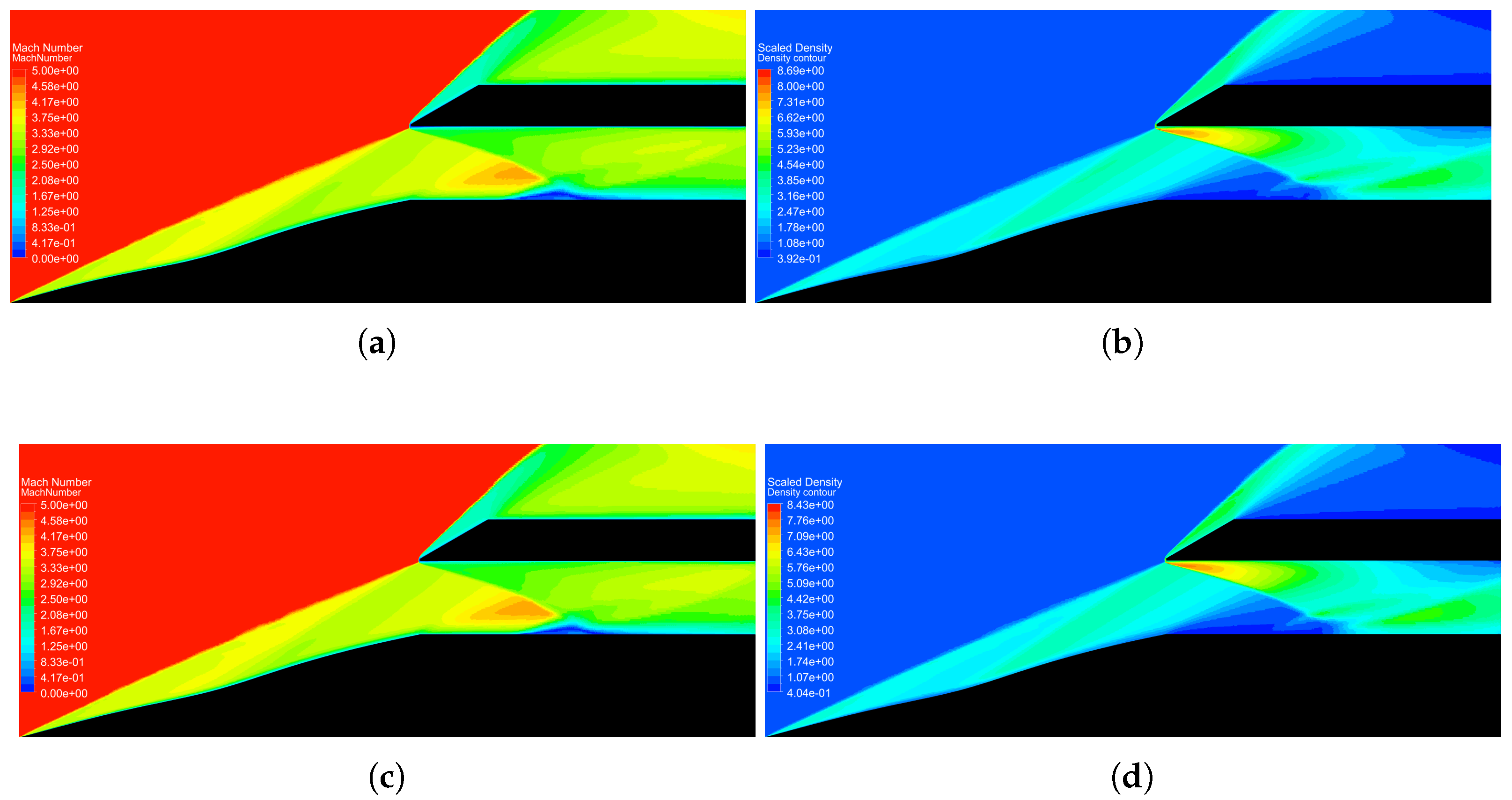
We now discuss the outcomes of the bi-objective optimization using the fitness functions $f_1$ and $f_3$. As previously stated concerning the Pareto front, the collection of optimum solutions collapses into a single minimum. However, the least drag optimal solution (minimum $f_1$) and the best TPR shape (minimum $f_3$) are presented for completeness and following the previous paragraph. The Mach and scaled density contours for these two configurations are shown in Figure 12. In particular, Figure 12a,b report the optimal drag solution while Figure 12c,d show the maximum TPR configuration. We instantly notice how nearly alike the two geometries are. As observed while commenting the $f_1/f_2$ optimization, the optimized ramp body is collapsed into a single continuous and regular surface, with the first ramp retaining the bulge and the second ramp exhibiting a slightly negative convexity. In contrast to the SPR optimum, improving the TPR promotes compression regularity and reduces the pressure jump between the ramp system and the duct entrance. Additionally, this example shows that the oblique frontal wave impinges nearly exactly on the cowl lip, thus minimizing normal shocks at the duct’s entry and recirculation/vein separation in this region. Examining the fluid dynamics inside the channel more in-depth, we see that the oblique wave reflection from the cowl lip impinges on the duct’s bottom surface and produces a tiny recirculation bubble. Nevertheless, this is restricted to a small region and the boundary layer may self-balance in a bit of space, indicating that the wave system is genuinely optimal and that detachments and recirculations result in confined and marginal occurrences relative to the system’s overall performance.

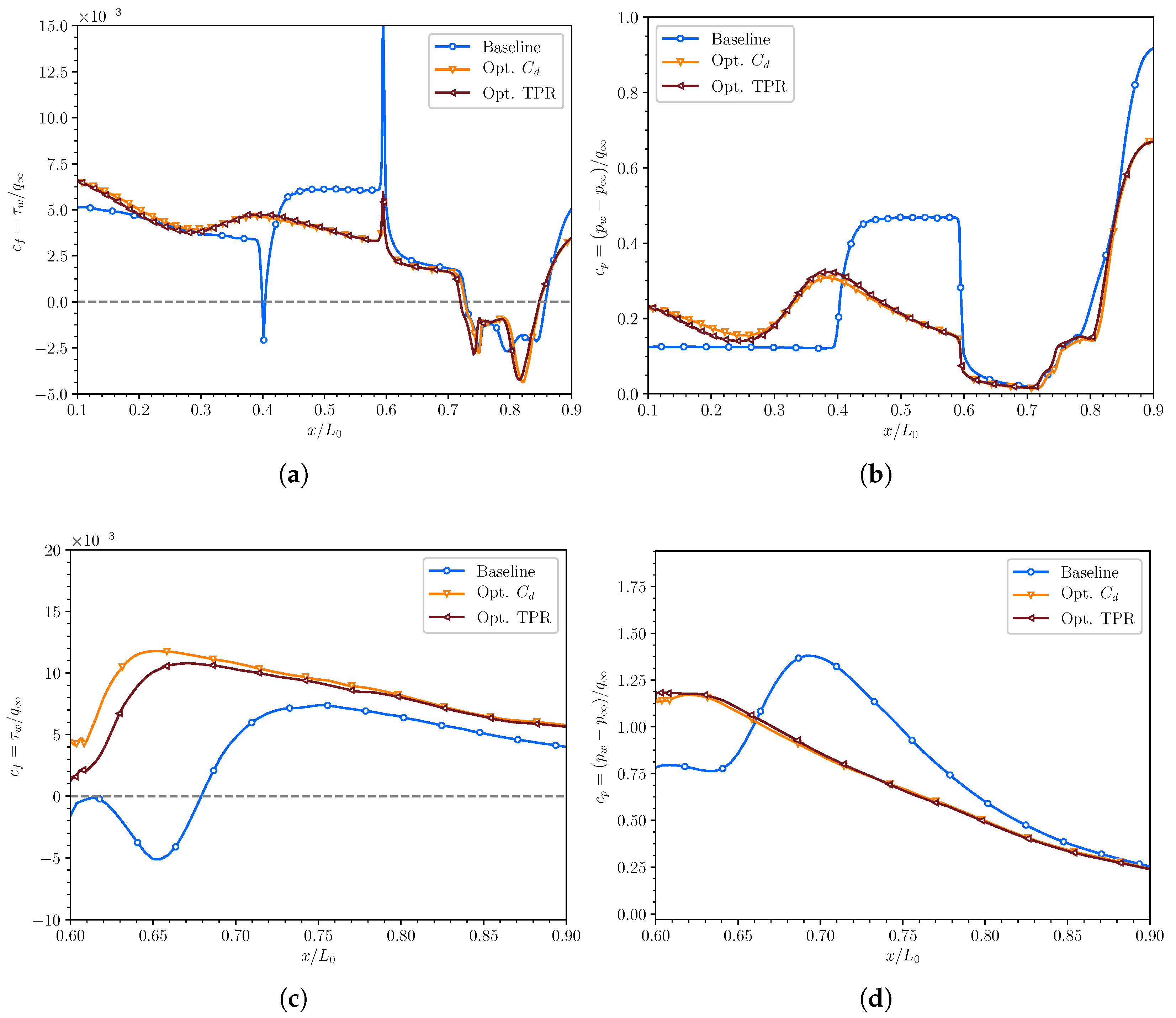
As usual, proceeding incrementally, we comment on the fluid dynamics improvement at the local level. Thus, Figure 13 shows the trend of the friction and the pressure coefficients along with the ramps and the lower surface of the intake channel (Figure 13a,b) as well as for the entire length of the upper internal surface (Figure 13c,d). The lines in shades of red still describe the trend for the optimized cases, while the blue curve reports the reference baseline values.

By examining the friction coefficient’s trend in Figure 13a, we see that the two optimal shapes provide identical outcomes. The wall speed gradient, in particular, stays almost consistent with the baseline scenario for the first segment of the first ramp. The bulge region then experiences a steady rise in friction, resulting in the boundary layer re-stabilization in a conventional turbulent configuration. Thus, the friction coefficient continues in a very delicate and regular manner up to the duct’s entry, when a slight speed gradient leap is noted due to the geometric discontinuity. In either scenario, the ramp’s trend is instantly restored up to the recirculation region due to the interaction between the oblique wave coming from the cowl lip and the boundary layer. In general, the recirculation region between the two ramps vanishes entirely, but friction stays much reduced over the whole length of the lower surface, particularly in the second ramp area. This results in a more gradual shift in the wall dynamics and, therefore, a more stable and efficient dynamic intake functioning.

The pressure coefficient’s trend related to the bottom surface (Figure 13b) is fascinating. We see that the dynamics have shifted dramatically compared to the baseline situation. The initial ramp experiences an expected pressure rise owing to the bulge, with a pressure peak on the wall about $0.4x/L_0$ as a result. The peak is rapidly evacuated due to the geometry of the second ramp, which in this instance has a little negative curvature, resulting in the flow gradually expansion. The trend is usually broken at the duct’s entry, where a net pressure decrease is recorded, although far smaller than in previously optimized circumstances. Pressure recovery is focused as necessary near the channel’s end, where the reflected shock wave causes the static pressure rise.

Rather than that, let us watch what occurs at the top surface. According to the friction coefficient (Figure 13c), any trace of flow separation is disappeared, and the flow may stay stable and adherent to the wall due to the impinging wave’s ideal location on the cowl lip. This is due to the wave potion being significantly advanced, as seen by the pressure coefficient trend (Figure 13c), which demonstrates how the pressure peak is greatly anticipated compared to the baseline setup, as well as of lower intensity.

Thus, on average, the geometric solutions produced by optimizing $f_1/f_3$ objectives exhibit features that are much superior to the baseline scenario and include elements of primary interest even when compared to the $f_1/f_2$ goals. We will proceed with the study by presenting the findings of the tri-objective optimization process, which prioritized the three factors simultaneously to identify the ideal geometries for the device under consideration.

5.2. Tri-Objective Optimization Results

Because the drag coefficient, the static pressure ratio, and the dynamic pressure ratio are all relevant characteristics of a hypersonic intake, the current section attempts to discuss the optimization outcomes that simultaneously includes all these three parameters; thus, providing a truly tri-objective optimal designing approach. It is important to note that, although bi-objective analyses have proven that drag and TPR are two entirely identical targets, nothing can ensure that a three-objective optimization would not provide contrasting designs by minimizing $f_1,f_2$ and $f_3$ at the same time. 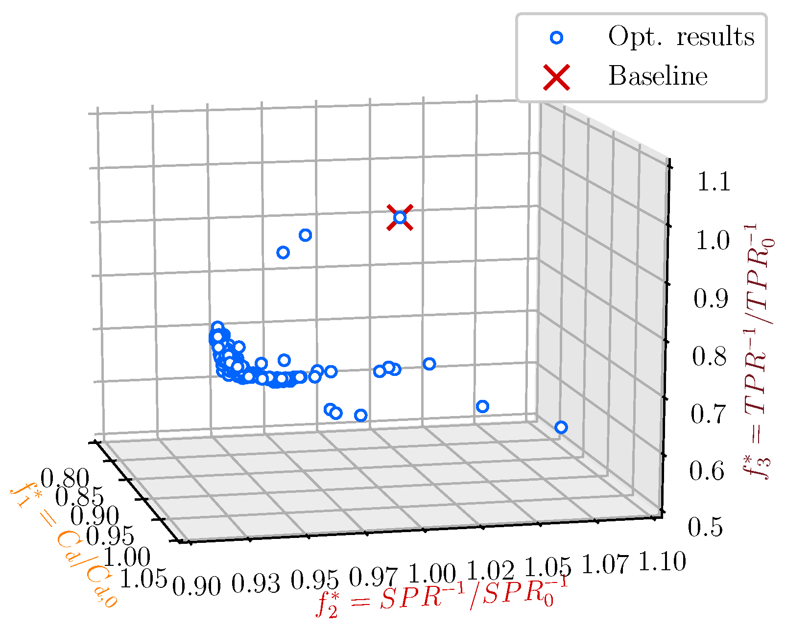Figure 14 shows the set of solutions obtained by solving Equation (3) while pursuing the objectives $f_1$, $f_2$ and $f_3$. For the purpose of completeness, Figure 14 report the result. The results compete with nInd = 6 evolved individuals for a number of nGen = 80 generations. Along the first coordinate the objective function $f_1$ scaled by the baseline geometry fitness, $f_{1,0}$, is reported as well as the $f_2/f_{2,0}$ and $f_3/f_{3,0}$ values are provided along the second and third axis, respectively. As a consequence, the three-dimensional box $[0:1]\times [0:1]\times [0:1]$ includes the set of Pareto-optimized solutions compared to the baseline setup.

We may quickly draw some conclusions based on these findings. Generally speaking, a three-objective problem yields a three-dimensional Pareto surface as a solution. Present computation, instead, clusters the optimal designs along a curve. Thus, results show that, even in a three-objective framework, one goal is redundant, and the optimization problem is genuinely bi-objective. In particular, as we noted in the bi-objected analyzes, we observe that the drag coefficient and the TPR allow for equivalent performance concerning the current device. Thus, minimizing the global drag or boosting the TPR yields comparable designs. Even if this behaviour had been observed in the previous bi-objectives analyses, the fact could not be asserted a priori for a tri-objective approach since non-linearity inherent to the system might have triggered the decoupling between the $C_d$ and the TPR parameters. However, the exceptionally high correlation between the two variables is easily explained. As previously stated, the drag coefficient and TPR are comparable pieces of information. The first describes how efficient a device is concerning the aerodynamic friction; the second is equal to one in the limit of inviscid and incompressible flow circumstances. Thus, optimal design options minimize recirculating flow portions or boundary layer thickening zones (drag information), probing the difference between an ideal and real viscous flow with shock waves (a TPR goal).

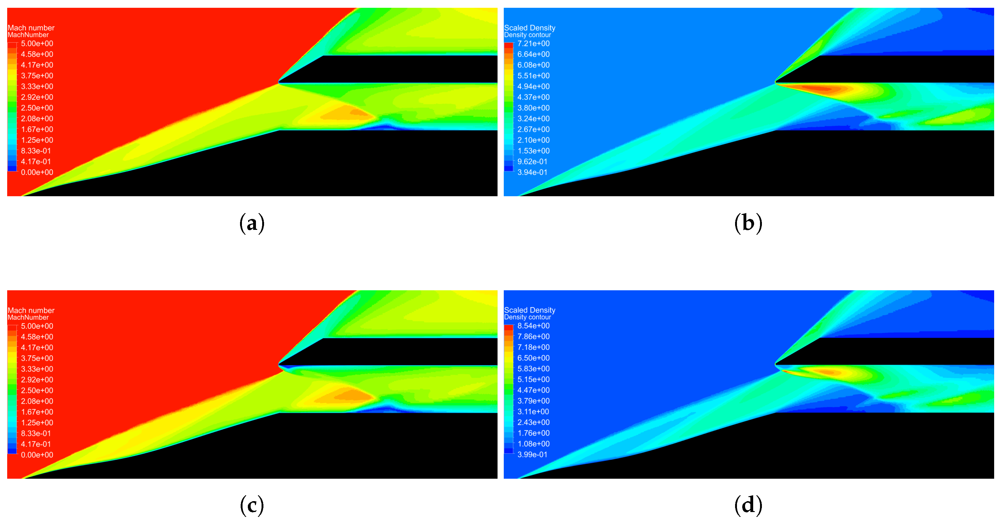
Let us now discuss the factors that contributed to the performance improvement. For conciseness, when it comes to fluid fields, we will look only at extremal instances with the least drag and the optimal SPR configurations. Figure 15 reports the Mach and scaled density fields associated with the extremal Pareto front solutions. Specifically, Figure 15a–d depict the stationary dynamics with the least drag and highest SPR, respectively. As the reader can notice, both cases show a relatively uniform and smooth ramp system, with a bulge in the initial ramp section and a subsequent negatively-convex second ramp. Such finding is a crucial difference between the two- and tri-objective approaches since the former optimization produced negative ramp curvature based only on the $f_1/f_3$ design objectives, while a positive convexity was reserved to the SPR boosting.

Both cases deflect the principal oblique wave to the cowl lip. The lowest drag design, in particular, reveals the primary oblique shock impingement location to exactly coincide with the cowl lip, whereas the maximum SPR configuration tends to shift it somewhat downstream in the channel, at the price of boundary layer stability. As already observed, both designs favour oblique reflections inside the channel. Such an arrangement minimizes losses due to entropy formation induced by normal waves and significantly reduces vein separation and boundary layer recirculation produced by the interaction of strong waves and solid walls. In comparison to the previous paragraph’s (especially concerning the lowest $C_d$ and highest TPR configuration), we can see that the geometry produced here is less exasperated in terms of the negative curvature of the second ramp, even though the position of the shock waves and the overall fluid dynamics are very similar.

We conclude by discussing the wall features associated with extremal instances. Figure 16, in particular, depicts the trend of the friction and the pressure coefficients along the dynamic intake’s bottom and upper surfaces, respectively. The blue line competes with the baseline reference, whereas the curves in shades of red reflect the parameter trends for the optimal configurations. We instantly see that, even on a quantitative level, curves corresponding to the least drag and the highest TPR are precisely overlaid, verifying our prior arguments.

The absolute eradication of the recirculation bubble between the ramps is still confirmed even for the tri-objective analysis, and a significant congruence between the different designs in the friction coefficients over the bottom surface is detected (Figure 16a).

The pressure coefficient trend over the lower surface (Figure 16b), instead, reveals a slightly higher pressure level for the SPR scenario compared to the other two configurations. The event is confined only in the second ramp region while externally curves overlap for all designs. We also notice that, when compared to the $f_1/f_3$ optimal setup, the pressure jump between the second ramp and the channel entrance is here more intense, indicating that the SPR objective plays a role in the geometries’ shaping, supporting the pressure level along with the ramp surface and keeping flat the pressure coefficient in this region.

By monitoring the trend of the friction coefficient over the top internal surface (Figure 16c), we draw similar conclusions to the two-objective analyses. In particular, optimizing the impingement location of the shock wave ensures that the flow stays fully attached to the wall, with only the configuration at maximum SPR exhibiting a tiny recirculation at the leading edge of the top lip. As it exits the channel, the trend of the optimized instances follows that of the baseline case.

Finally, the pressure coefficient on the lower surface (Figure 16d) exhibits the typical peak at an advanced position compared to the baseline scenario. The peak intensity is much lower for the least-drag/maximum-TPR case than those with maximum SPR.

5.3. Role of Cowl Lip Location

In earlier sections, we discussed the role of compression ramp design without looking at the influence of the intake cowl lip. Indeed, we are well aware that the lip location and shape heavily impact the aerodynamic efficiency of such devices. Thus, the present section aims to parametrically explore the lip location’s role concerning the tri-objective optimized designs obtained in the early campaign: therefore, looking at the role of the lip location concerning the optimal $C_d$ and the optimal SPR cases. In particular, we attempt to shift the lip back with respect to the baseline geometry and we compare three different configurations, namely moving the lip by 1%, 3% and 5% downstream the original location. Percentages refer to the intake chord length.

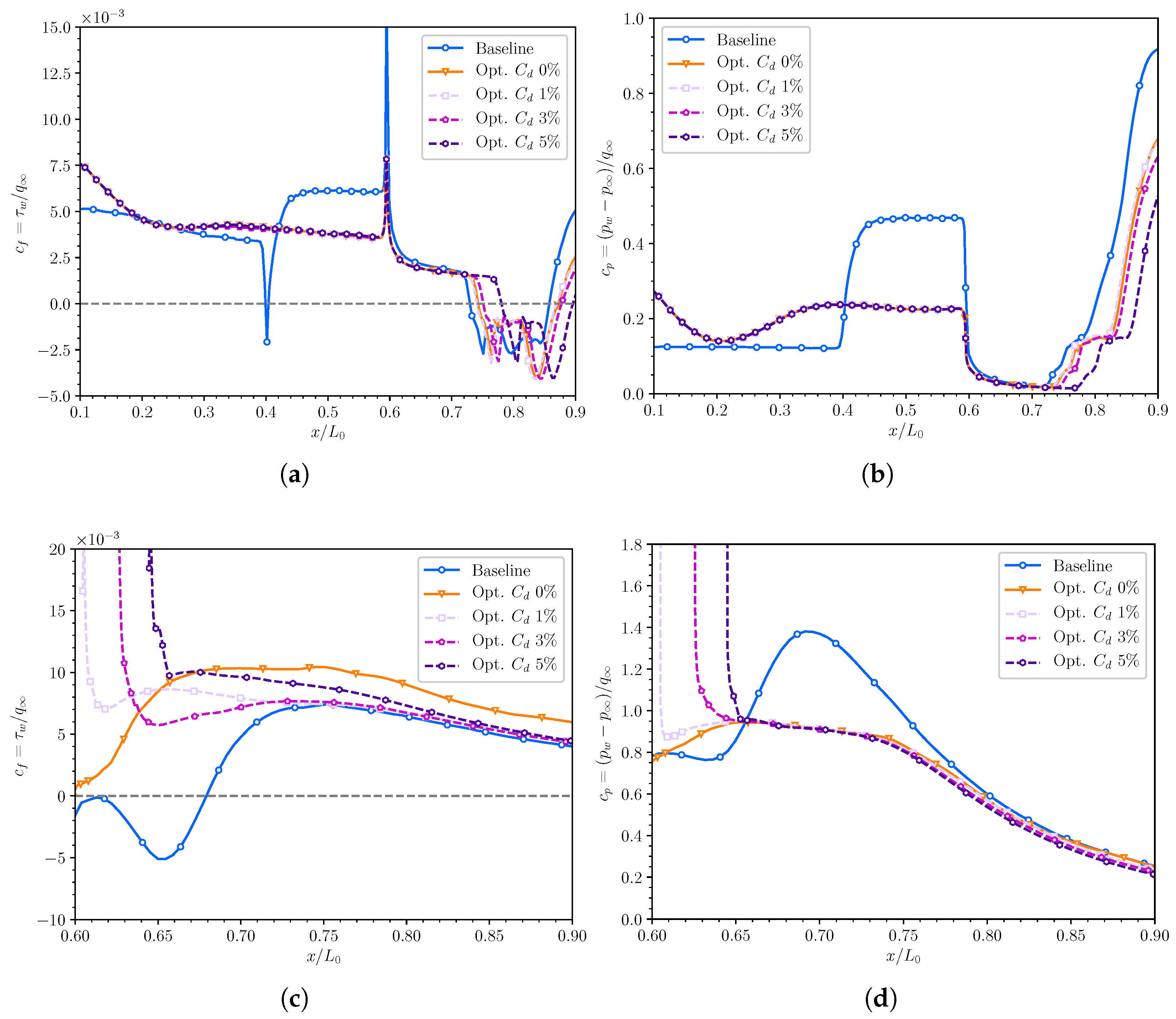
Figure 17 reports the aerodynamics coefficients results, $c_f$ and $c_p$, concerning the three optimal-drag-derived geometries with backward lip. In particular, figures still provide the baseline solution in blue while the optimal reference is reported with its orange line. Lip-backwards designs are reported in shades of purple. As the reader can notice, minimal discrepancies can be detected between the reference and the lip-shifted solution concerning the lower surface aerodynamics (Figure 17a,b). In this respect, we remark that when the cowl lip is retracted, the recirculation bubble naturally moves downstream since the flow separation due to the oblique shock propagating from the cowl lip moves accordingly with the lip. The location of the incident wave’s also has a negligible effect on pressure recovery, which is somewhat advanced relative to the configuration with the lip in the nominal position.

On the other hand, the top lip location influence is less negligible on the upper surface. The friction coefficient (Figure 18c) shows that retracting the lip stabilizes the boundary layer. A monotonically decreasing $c_f$ trend, in fact, is detected, mostly regardless of the amount of retraction. The lip shifting also allows the boundary layer to transit immediately to a fully turbulent regime, while the nominal location exhibits a partial friction rise owing to a laminar-to-turbulent boundary layer transition. The pressure coefficient’s behaviour (Figure 18d) confirm such behaviour, exhibiting a constant monotonous trend where the lip is set back. Thus, the arrangement avoids pressure gradient inversions resulting in detachment phenomena, thereby increasing the intake’s operating envelope, particularly in off-design conditions.

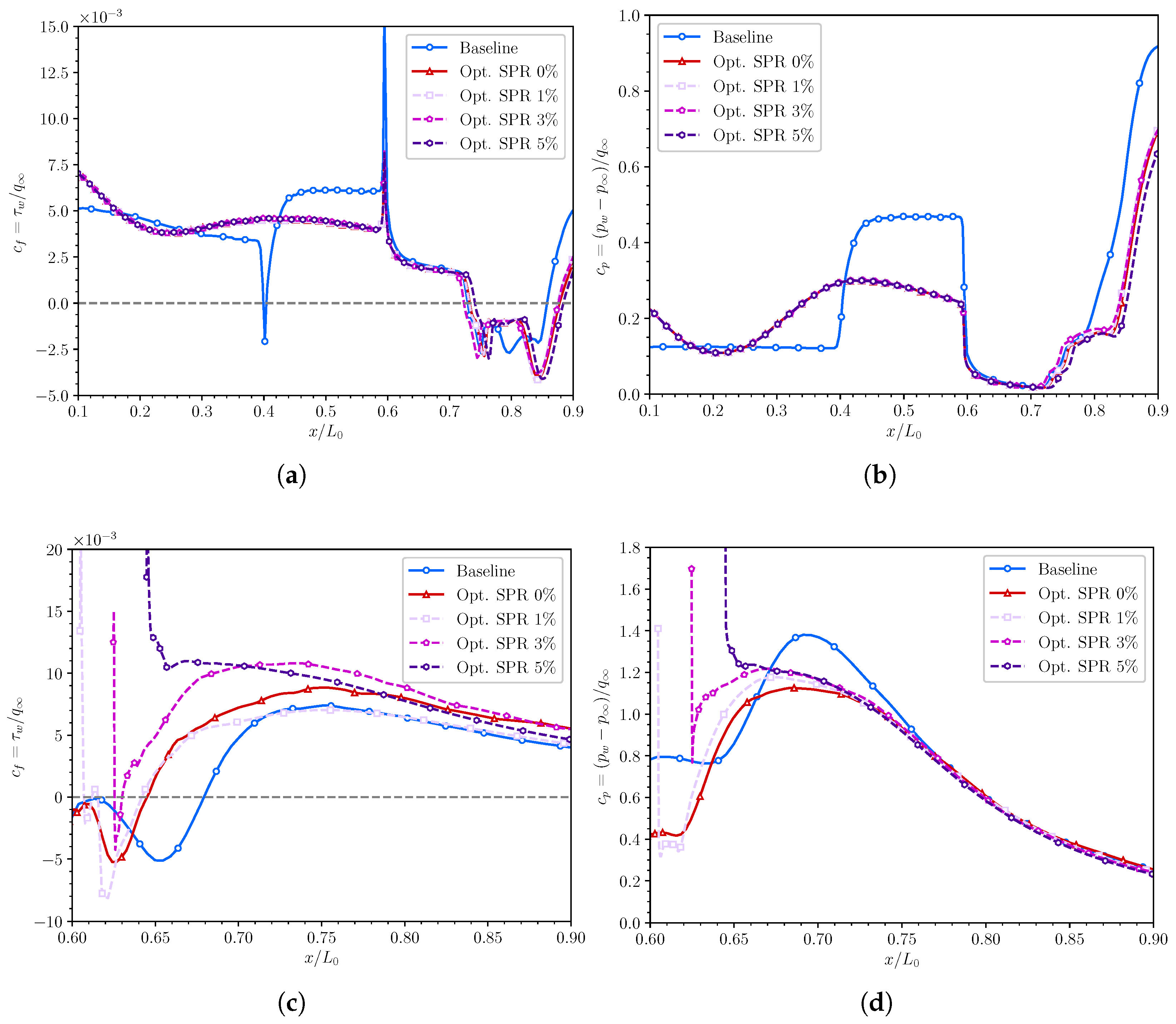
For completeness, lip retraction is also investigated for the SPR-optimal design case. The trend of the aerodynamic coefficients along the surfaces of interest is reported in Figure 18. Again, the baseline solution is drawn with a solid blue line, the SPR optimal solution recovers its red tone while shades of purple present the SPR-optimal-derived configurations with the top lip at a rearward position of 1%, 3%, and 5% of the intake chord, respectively. Again, the lip location induces negligible effects in the lower wall aerodynamic coefficients (Figure 17a,b), with findings that are entirely consistent with those previously explained. Top wall performance is much more intriguing (Figure 17c,d). Even in this scenario, in fact, the location with the greatest retraction, i.e., 5%, removes any trace of boundary layer separation or transition, resulting in a perfectly monotone trend of the friction coefficient. Similarly, the pressure coefficient is exceedingly regular, avoiding adverse flow pressure gradient components.

Finally, in terms of the analyzed intake geometry, retracting the cowl lip favourable influences flow. In particular, for both the studied configurations, it is observed that the rear position of the upper lip minimally influences the lower channel surface fluid dynamics while it acts more markedly on the boundary layer relative to the upper wall. More rearward positions show friction and pressure trends of a more markedly monotonous character with consequent optimization of the intake envelope regime in off-design conditions. However, a more systematic quantification is required to make solid conclusions.

6. Conclusions

The present work presents a systematic and straightforward numerical approach for the automatic design of super/hypersonic inlet intakes in a multi-objective optimization framework. The compressible RANS equations forecast system dynamics in various configurations, the latter built up via genetic algorithm combinations. CFD databases enable novel inlet shapes based on precomputed design objectives. The process embeds non-linear flow characteristics and viscous phenomena as crucial aspects of engineering prototyping from the beginning of the design process.

First, the numerical model is validated in grid resolution and turbulence model sensitivity to establish the optimal numerical assessment. As a result, an extensive validation campaign is reported for global and local quantity convergence, determining the minimal mesh size and the appropriate turbulence model for system dynamics prediction. According to our analyses, 300 k elements coupled with k-$\omega$ SST provide a good balance between computational time and accuracy.

The optimization process minimizes the drag coefficient while boosting the static and total pressure ratios. The first parameter concerns the geometric interference of flying vehicles with respect to the freestream flow, the second targets flow compression for the inlet intake, the latter disfavors normal shock waves and viscous phenomena due to the incremental contribution of oblique wave trains and adherent boundary layer. The three parameters’ role is systematically investigated by first attempting a series of bi-objective optimizations and then integrating them into a single designing process. The analyses revealed that the drag coefficient and the total pressure ratio are completely equivalent performance parameters so that the minimization of the first or the maximization of the second lead to identical designing shapes.

Numerous comparisons and comments are made between the optimal shapes configurations. The analyses, in particular, focused on the physical reasons underlying the obtained improvements, attempting to understand the benefits introduced by the optimized geometries compared to the baseline setup. Qualitative (i.e., observation of fluid fields) and quantitative results (i.e., analysis of the friction and pressure coefficients along the walls) are provided.

Finally, the effect of cowl lip placement is explored at a basic level by examining the influence of a rearward position for optimum drag shape. The investigations revealed that retracting the cowl might increase the boundary layer stability over the surfaces within the intake channel.

Based on the limitation of RANS modelling, future research aims at performing wall-resolved LES of the optimal intake designs here determined. LES modelling, in particular, has been already successfully employed by the research group and the reader should refer to De Vanna et al. [19] for a complete characterization of the methodology. In addition, combining GA with high-fidelity computational fluid dynamics methods such as the wall-modelled LES approach proposed by De Vanna et al. [54] will be a goal in the near future.