Abstract
This work aims to analyse different injection configurations for the analysis of the emulsification process in a Y-junction staggered horizontal pipeline. The case study comprises a multiphase analysis between two liquids, one with high and the other with low viscosity. Through numerical simulations, it is intended to explain the behaviour and describe the mechanism that produces the water–glycerol emulsification process with three supply zones for both fluids. According to the phase injection scheme, six input scenarios or combinations were analysed. Through strain rate and shear velocity analyses, it was possible to describe the early stages of the emulsification process before a flow pattern is constituted. The results show significant variations concerning the high viscosity fluid, mainly because it presents a partial pipe flooding, even in the injection zone of the low viscosity fluid. The fluid ratio varies according to the input position of the phases. Additionally, a smooth blending process was observed in some scenarios, due to the fact that the continuous phase gradually directs the main fluid to the pipeline centre. The analysis revealed that supply configuration has a significant relevance on the development of the main fluid flow and a substantial extent on the emulsification process.
1. Introduction
In the oil and gas industry, there are significant challenges in maintaining hydrocarbon production. Among the most prominent issues, the optimal transport of these products stands out. Due to the implications of long-distance transportation, the flow of oil–water mixtures in pipelines has received a lot of interest. The study of the two-phase and multiphase flow has grown specifically to enhance and make the transportation of the products more profitable [1,2]. In order to optimize production, accurate knowledge of the behaviour of oil and water in pipeline flow is essential [3,4]. This is strictly entailed to the pressure drop caused by their higher viscosity [5,6].
Another reason for this growing interest in this industry is the notable increase in the management of two-phase flow due to the fact that some oil fields are at the end of their useful life and the oil–gas and water ratio changes, so the flow that is conducted in the pipes as well as their composition, are different from the main design.
Water injection is a way of reducing pressure drop that aims to create core annular flow [7], i.e., a flow regime defined by the presence of an oil core enclosed in a water annulus wetting the pipe wall, lowering the apparent viscosity of the mixture significantly. For example, Wang et al. [8] investigated the flow characteristics of two-phase heavy crude oil–water flow. Oil-water emulsion dispersed flow, intermittent flow and partially segregated water layers, water stratified flow, water semi-annular flow, and water annular flow were observed in their study. However, a briefly physical mechanism was explained.
Flow patterns in high viscous oil-water two-phase flow were investigated by Bannwart et al. [9] specifically in the horizontal pipes. They observed stratified, bubbly stratified, dispersed bubbles and annular flows. Within stratified flow patterns, the pipe upper walls were constantly lubricated by water, which was attributed to interfacial phenomena and the wettability effect. A slight reason for this natural behaviour was explained.
This bias in the analysis of results is completely understandable given that the measurements must be made using non-invasive methods, since doing so would compromise the results and contribute to the formation of other types of flow patterns. On the other hand, the oil industry has dedicated a large amount of resources to try to simulate multiphasic flow in pipes, as in the case of the Barcelona Supercomputing Centre [10,11], Schlumberger Research Centre in Cambridge, England and the Schlumberger Riboud Product Centre in Clamart, France, and who has published articles related to this topic.
Computational analysis tools, CFD, have been very helpful in revealing the physical mechanisms that directly influence the formation of these flow patterns. However, to be able to represent numerically the very nature of this type of flow is sufficiently complicated as is the solution of advection–diffusion equation [12]. For this reason, the use of High-Performance Computing [13,14] has been increasingly used. In this area, there are investigations in the open literature, which, although they are very complete, are limited by the computational performance. A proof of this is the investigation of Rodriguez and Baldani [15] who conducted experiments on two-phase liquid–liquid flows. They collected and analysed pressure gradient and holdup data with emphasis on the stratified flow pattern. Using a CFD commercial code, they conducted numerical simulations for a simplified liquid–liquid pipe flow with non-interfacial dispersion. In that study, the numerical simulations captured the interfacial waves observed in experimental video recordings and images. Particularly, the qualitative and holdup predictions of the CFD code were good, however, the pressure gradient predictions were inaccurate.
Y-junction staggered horizontal pipeline is the most common confluence configuration in which the most operative problems have been detected because the mainstream is directly affected by lateral or alternating streams. For this reason, it is of great interest to analyse the effect that alternating streams have on the development of the main flow during the confluence when different types of fluids, as in the case of oil and water, converge. Therefore, the aim of this study is to analyse different injection configurations in a multiphase system that give rise to water–glycerol emulsion mixture, increased fouling and clogging in a Y-junction round horizontal pipe. To conduct the research, it is used the Fluid Volume (VOF) method, which is a popular Computational Fluid Dynamics (CFD) study model for multiphase studies. Through strain rate and shear velocity analyses, it is possible to describe the early stages of the emulsification process before a flow pattern is constituted and describe the above-mentioned effect.
2. Experimental Setup
Figure 1 shows the complete experimental setup rig. The pipeline is located at the Engineering Institute-UNAM and was designed to evaluate the flow properties of liquid–liquid and liquid–air mixtures constituted by high-viscosity liquids, i.e., heavy and extra-heavy crude oil. The data used for this analysis were taken from the experimental rig described in [16,17] under the P1 sensor.
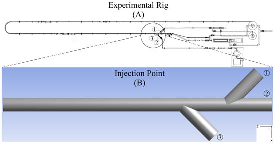
Figure 1.
Top view of the complete experimental rig setup (A), injection point close-up (B). (1), (2) and (3) phases nozzles.
As part of the development of numerical simulations, it is necessary to discretize the geometry or computational domain explicitly to focus computational resources. For this reason, the Y-junction supply system was selected and marked as Injection Point, illustrated in the close-up Figure 1B. Further details are described in [16].
3. Numerical Setup
3.1. Case Study
The numerical model considers staggered Y-joint nozzles with 25 cm of separation between each other and with an inclination of 45°. The pipe diameter, D, for all injectors is 7.62 cm with a total length, L, of 150 cm. A two-phase water-glycerol 3D simulations were performed using a commercial CFD software ANSYS Fluent v13 academic license in a Xeon 32 cores Workstation and two high-performance GPUs, Nvidia Quadro 6000 and a Tesla C2075 to accelerate calculation. The numerical domain is detailed as a horizontal Y-junction pipe with three incorporation zones for both fluids. The inlet mass flow is constant, for both phases is 5 kg/s which is distributed symmetrically between the injection pipes according to the study scenario. All the thermodynamic properties are shown elsewhere [17]. The injection zones have a separation distance to avoid agglomeration or collision between the inlets with the intention of minimizing high turbulence and thus avoiding areas with eddies or swirls over the main flow. According to the phase injection scheme, six input scenarios or combinations were analysed. Three cases for the incorporation of the low viscosity fluid through two alternate supply zones and three other cases for the high viscosity fluid, respectively. The numerical simulations test matrix is listed in Table 1.

Table 1.
Phases injection input scenarios.
3.2. Numerical Domain Details
A hybrid of advancing-front meshing [18] and the Cut-cell method [19] was used to construct the numerical domain mesh. The advancing-front method has advantages over common grids, such as facilitating tessellation in geometrically complex domains and allowing the mesh density to be adjusted. The complexity of the geometry, specifically at the Injection Point, lies in the staggered nozzles, an area to which the Cut-cell mesh must be adapted, as illustrated in Figure 2. The combination of these two methods is used to obtain a constant growth of thin layers and cells from the pipe walls to the domain’s edge, allowing a good representation of the physical phenomenon, particularly when high-order discretization schemes are used.
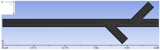
Figure 2.
Refinement of the Cut-cell type hexahedral mesh for the injectors.
The boundary conditions used in the simulations consider adiabatic and non-slip, combined with enhanced wall function to correct any miscalculation near walls treatment. For the phases’ injection, a mass flow condition was used in each nozzle. For the outlet limit, the discharge occurs in atmospheric conditions of 1 atm of pressure and 293 K of temperature.
3.3. Numerical Discretization
The numerical simulations were discretized as follows. For pressure spatial discretization the PRESTO Scheme (PREssure-STaggering-Option) [20], a third-order MUSCL (Monotonic Upstream-centred Scheme for Conservation Laws) [21] for momentum solution and the modified HRIC (High-Resolution Interface Capturing) [22,23] for the volume fraction reconstruction. Furthermore, for the pressure–velocity solution method, a fully coupled scheme was implemented. The results show that the high-order MUSCL method, effectively reduces numerical diffusion, leading to better resolution of multiphase flows compared to first-order methods. Furthermore, the PRESTO and HRIC with the pressure-velocity fully coupled exhibit superior convergence compared to other alternatives.
In addition, an adaptive time step was considered for the numerical simulations in order to ensure that the time step was correct in these types of multiphase simulations. The time interval must be small enough to resolve time-dependent characteristics and guarantee convergence within a maximum number of iterations. The time step, , is calculated using the equation,
and the values considered in the simulations have the order of .
For tracking the surface of the two immiscible fluids, the most suitable multiphase model is the so-called Volume of Fluid (VOF, or surface-tracking technique), mainly due to the consideration of the hydrodynamics of the water-glycerol flow in this study. In this method, the phases are treated as continuous and prevent the phases from being interpenetrating. Furthermore, in this model, the phases are considered as isothermal, transient, without mass transfer or phase change. For this reason, each of the considered fluids shares a single set of momentum equations and the volume fraction of each of the fluids in every computational cell is tracked throughout the domain.
When using the VOF model, considerations must be set forehand to give a suitable numerical representation. In other words, in each control volume, the volume fractions of all phases must sum to unity. As long as the volume fraction of each phase is known at each location, the fields for all variables and properties are shared by the phases and represent volume-averaged values. Thus, depending on the volume fraction values, the variables and properties in any given cell are either purely representative of one of the th-phases, or representative of the phases’ mixture,
Based on the local value of the phase the appropriate properties and variables will be assigned to each control volume within the domain. In this study, the primary phase is water, .
3.4. Governing Equations
The solution of the continuity equation for the phase volume fraction allows the tracking of the interface between the phases, and is given by:
where is the density, the velocity vector, the time and due to the no mass transfer assumption. For the interfacial tracking, glycerol as the secondary phase, , is achieved by finding the solution of the Equation (4) for , thus,
.
Therefore, from the aforementioned considerations, the volume fraction of is computed from the relation .
As the resulting velocity field is shared between the phases, only a single momentum equation is solved for the entire computational domain, which depends on the volume fractions of all phases through and .
where, , , and F are pressure in the flow field, viscosity, acceleration due to gravity and the body force, respectively. On the other hand, and are estimated by using, and .
3.5. Interfacial and Surface Tension Treatment
A piecewise-linear technique is used by VOF to build the interface between the fluids. Within each cell, it is assumed that the interface between two fluids has a linear slope. This linear shape is used in the system to calculate fluid advection via the cell faces. The position of the linear interface relative to the centre of each partially filled cell is computed in the first step of interface reconstruction using the volume fraction and derivatives information in each cell. Then, using the computed linear interface representation and information about the normal and tangential velocity distribution on the face, the fluid advection through each face is estimated. Finally, using the balance of fluxes calculated in the preceding step, the volume flux in each cell is calculated.
In addition, surface tension along the interface between the phases is accounted for in the VOF approach. The model specifies the contact angle between the phases and the wall, and the surface tension coefficient is assumed to be constant. To do so, the continuum surface force model [24] is used in the surface tension model. When the surface tension is included in the VOF calculation, a source term, F, appears in the momentum equation at which the pressure drop across the surface can be calculated using the surface tension coefficient, and the curvature, , of the surface can be estimated using the Young–Laplace equation and two radii in orthogonal directions R1 and R2, defined as . As a result, the pressure drop across the surface may be used to describe surface tension. The source term for two-phase water–glycerol is then written as:
3.6. Turbulence Model
Turbulence models must be addressed in numerical simulations of multiphase flow if one or more of the phases are in the turbulent regime. The Shear Stress Transport (SST) turbulence model [25], which is based on the Reynolds Averaged Navier–Strokes (RANS) technique, was utilized in this study because it has some advantages referring to high viscosity water–glycerol flow [26]. Specifically, it is implemented to facilitate the prediction of the initiation and magnitude of flow separation under unfavourable pressure gradients by including transport influences into the eddy–viscosity representation over the turbulence models. It also gives some improvements on the free-stream independence in contrast to the model. The model is given by,
The term represents the production of turbulence kinetic energy due to mean velocity gradients; the generation of : and the effective diffusivity of and , respectively; and the dissipation of and due to turbulence, respectively; the cross-diffusion term; and are user-defined source terms. The effective diffusivities for are the same as in the standard model.
3.7. Sensitivity Analysis and Validation
Finally, four versions of the mesh were built in order to obtain numerical results independent on the mesh. In Figure 3, it can be observed the deviations of the results for every mesh version. The data were taken from the results obtained through a central line or central marker of the pressure gradient along with the calculation domain and thus, the sensitivity analysis could be carried out.
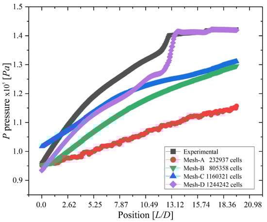
Figure 3.
Pressure plot, values along the central marker. Experimental data obtained from [17].
It is observed that Mesh-A greatly underestimates the pressure values, indicating that the representation of flow, that is, hydrodynamics, was correctly modelled, but the precision of the values is precarious compared to Meshes -B, -C and -D. On the other hand, Mesh-B still underestimates the pressure values in comparison with the experimental data. Although the number of cells is just over three times the number of cells in Mesh-A, 44% less than Mesh-C and 54% less than that of Mesh-D, the results are still far from those of experimental. In the case of Mesh-C, it shows an area with values already close to the experimental ones with a deviation of 22%, which is still unacceptable due to the required precision of the results.
Finally, Mesh-D shows a deviation of 9.98% with respect to the experimental results just in the area of the injectors and as the flow develops it stabilizes, obtaining a deviation of 0.23% before . It is noteworthy, that a more refined mesh beyond this Mesh-D number of cells is not feasible due to the computational resources, which could derive in unreachable time convergence, entering on the LES refined meshes type, for which another type of model and discretization is needed to get convergence. Therefore, Mesh-D was used, since the greatest precision of the results is necessary and convergence time reachable to be able to describe the mechanism that gives rise to the emulsion mixture.
4. Results and Analysis
For this particular water-glycerol study, water is considered as the transport phase or continuous phase, while glycerol is the dispersed phase. The evaluation of the fluid will depend on the properties of the continuous phase within the VOF model. With the aforementioned, the study of the evolution of the water–glycerol emulsion will depend on the calculation and the results obtained from the behaviour along with the calculation domain of the continuous phase. Therefore, three stripes called markers were selected within the computational domain, which are represented by three straight lines starting at the inlet of the numerical domain until the outlet boundary, which are named as: right lateral line located at ; left lateral line at and; centre line at. The location was selected because, in general, they are located where emulsification might arise and especially because the central marker cannot give enough information about what occurs in the injection zones. For the analysis of results, the strain rate, , and the shear velocity, also called friction velocity, , were selected.
4.1. Strain Rate Analysis
In multiphase systems, is often used to quantify the intensity of mixing and the behaviour between fluids when they interact. The strain that fluid layers undergo due to impact, collision or rubbing reveals the nature of mixing. When has several orders of magnitude compared to of the global development of the fluid, it is known that there is a mixture or mixture in development and the amount or value of that magnitude gives the hint of being a mild or violent mixture. For each case analysed (Figure 4), it can be seen that the phases’ injection scenarios play an important role to achieve emulsion since changes substantially.
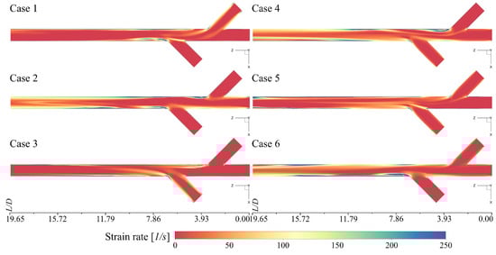
Figure 4.
Strain rate contours of the different injection scenarios.
The contours of are shown in Figure 4. These contours are arranged on the ZX central plane to better appreciate the development and evolution of the phases and their own interaction. There is high inherent to the geometry corners, specifically those that intersect with the main pipe. Since the lateral tubes have the function of injectors towards the main pipe, the intersections are those that present the highest regardless of the geometry. In this study, the junctions are not the exception, for this reason, they show sufficiently large values with which the analysis of the fluids and their development is neglected since they are produced exclusively by geometry.
However, when analysing the values obtained from the contours of , the path that the conjunction of the fluids has (before emulsion) is better distinguished. Although the emulsification process is given only by the properties of the fluids and their interaction in the injection zone, it is no ruling out the influence it receives from the geometry, in particular of the staggered injectors.
In every case, the strain rate reveals the bulk fluid trajectory, but cases with major differences are noted. At a first glance, two scenarios can be differentiated, 1 and 3. After , the deformation that comes from the geometry corners starts to diminish, giving the appearance of a smooth phases blend. Nevertheless, in Case 3, higher values >250 [1/s] can be distinguished. These can be products of the swirl, eddies, or turbulence within the fluid interacting with the pipe walls as studied Soleimani et al. and Meher [27,28].
In Case 2 and 5, a straight bulk fluid development can be observed from the inlet boundary until the outlet boundary with no perceivable major changes in the main flow direction. This behaviour is due to the fact that the injection of the same phase through the lateral pipes or nozzles pushes the central fluid, resulting in a directed flow. However, the values are different because the lateral input fluid is different, therefore Case 2 shows higher values. This indicates that the glycerol diffuses or disperses over the water flow, while in Case 5, the water that enters through the main or central pipe only directs, in general, the development of the bulk fluid.
Now, the values of in Cases 4 and 6 are greater than Cases 1 and 3, respectively, since the injection of the phases is the inverse. The change in the procedure in which the fluids are supplied has a great influence on the mixing process and in these cases the manner in which the bulk fluid is transported and diffused along the pipeline. Furthermore, in all cases, values of indicate that a swirl might be developed driven by a greater quantity of the same phase loaded on one side of the main pipe, specifically Cases 1, 3, 4 and 6.
In Figure 5, the values of the markers are shown in the scatter plot. In the same way as in the analysis of the contours of , in the scatter plots, it is possible to recognize differences between the case studies. In the first place, Cases 2 and 5, the shear velocity does not exceed , indicating that, at least in the location of these three markers, the mixture is smooth which is characterized by the amount of fluid coming from the lateral injectors and directs towards the centre of the main pipe concentrating the bulk fluid. Secondly, Cases 1 and 4, whose development is influenced by the left-loaded fluid. As there is more of the same fluid on that side of the pipe, it is noted that the fluid behaviour will be substantially affected until there is sufficient development and distribution along the pipe. This is demonstrated because just after is when the disturbances occur. Finally, although in Cases 3 and 6 the disturbances also begin at , they are of greater magnitude . This is essentially due to the fact that, regardless of the fluid that enters through injector 3, it receives the direct impact from the other inlets.
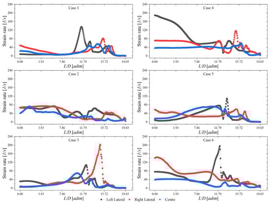
Figure 5.
Strain rate values over the three different markers of the distinct cases.
4.2. Shear Velocity Analysis
When the mixing mechanism involved occurs between thin layers, the analysis of the density profile is not sufficient for the accurate identification of disturbances attributed to the behaviour and interaction of the phases. A second analysis should be performed using a relation between the shear rate of these layers and their location to identify instabilities. A shear velocity is used in its simplest form to understand the development of bulk fluid flow. A velocity scale to represent shear strength is called a shear velocity, . This velocity scale or friction velocity characterizes the shear in a boundary or in a layer. In this analysis, the shear rate of the mixing/blending layer [29,30] is defined as , where is the shear stress and is the mixture density.
The identifies the disturbances or in this case the relative displacement between the phases that give rise to the water–glycerol mixture as an emulsion. In this way, by taking into account the , it is possible to identify at what intensity it is that the fluids collide and diffuse among themselves. The disturbances’ intensity is a direct reflection of the emulsification process, which helps to locate the area with the dominant relevance for diffusion along the pipeline. This process can only be accounted for when the fluids are assumed immiscible since otherwise, the inter-diffusion for the mixing process prevents the intensity of the mixing mechanism from being appreciated.
Most of the correlations for obtaining the mixture assume the complete or developed emulsion and account for the proportion of glycerol in water, but do not indicate how this process is or the intensity with which such mixing is carried out.
If the is large, this indicates that the upper layer, or in this case, the layer furthest from the walls of the pipe, is sliding on itself and towards the centre of the pipe, since there is resistance to flow either due to adhesion, friction due to roughness or because there is an obstruction pressure. This development can be observed in the central section of the numerical domain in the form of an annular flow. This is mainly due to the fact that when glycerol collides with water, the latter drives the more viscous fluid, forming an instability that gives rise to the first moments of emulsification. On the other hand, when means that both fluids are moving at the same relative velocity.
Figure 6 depicts the contours of . These contours are placed on the ZX central plane to recognize the phases’ advancement, as well as their interaction. When examining the cases by supply configuration of the phases (1, 2 and 3), it was detected that two of the cases had a similar development of the main flow. Cases 1 and 3 stand out because, in both, the is able to stabilize between and with . In these cases, the water supply is loaded towards the sides of the pipe, left and right, respectively, achieving a smooth mixing in early zones after the junctions, also called liquid holdup. Case 3 stands out since it manages to obtain low values of , which indicates that its disturbances are less and the mixing process is driven by the water supply, followed by Case 1. This is due to the fact that the water that is introduced by nozzles 1 and 2 pushes enough glycerol gradually forcing it to flow as shown by the strain rate graph, respectively.
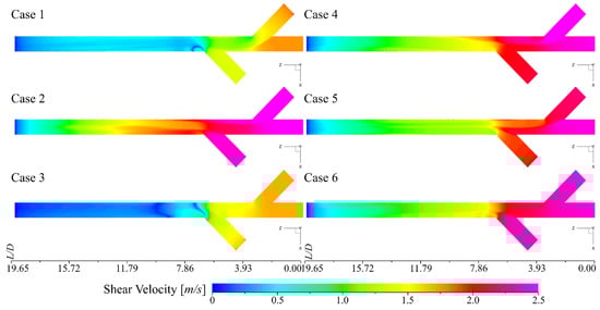
Figure 6.
Shear velocity contours of the different injection scenarios.
For Case 1, this is somewhat more forced since the water is supplied by nozzles 2 and 3. With this change in the water supply, the glycerol flow development is driven by the water coming from the main pipe and subsequently displaced by the amount of water that is supplied immediately after the nozzle 3. This causes two areas of interaction for the emulsification process. In contrast, Case 2 is the opposite.
Case 2 shows a more aggressive development in the sense that the does not stabilize, but almost reaches the outlet boundary of the numerical domain, particularly at . This indicates that the mixture is directed by the central supply, but is forced to flow only through the centre, preventing the glycerol from getting too close to the pipe walls.
On the other hand, Cases 4, 5 and 6 have a very similar development. By carefully evaluating the contours of , it could be observed that there are also traces of the path that the phases follow in the development of the main fluid and before the mixing or emulsification process. In these 3 cases, the gradual stabilization begins from manifested by the rapid decrease in the magnitude of . The behaviour is better recognized by observing the values obtained through the markers.
The scatter plots are shown in more detail in Figure 7. The Case 1 scatter plot shows a staggered behaviour which corresponds to the location of the supply entrances. Then, the values tend to decrease because the main fluid is already mixed or the phases have the same relative velocity, developing a complete emulsification process.
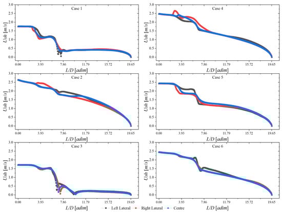
Figure 7.
Shear velocity values over the three different markers of the distinct cases.
The Case 2 scatter plot corroborates the aforementioned contour analysis. The emulsification process is much more aggressive since perturbances decrease while the main flow develops. In Case 3, a suddenly staggered decrease of is observed after and reaffirms the contour analysis. Finally, for the remaining Cases, the progressive decay without major disturbances is inductive that the emulsification process is gradually progressive and to a certain extent, smooth or delicate. These are achieved with a location after in each of the cases.
5. Conclusions
In the present study, different injection configurations were numerically analysed for the description of the emergence of the emulsion mixture development in pipelines. Six different phase supply configurations were described in a horizontal Y-junction pipeline. The results show significant variations concerning the high viscosity fluid, mainly because it presents a partial pipe flooding and clogged by the phase loaded to one or the other side of the pipe, respectively. Cases 2 and 5, show a better fluid development caused by the relative confinement to the pipeline centre driven by the phases’ supply configuration. Case 3 has the smoothest blending process due to the fact that the continuous phase gradually directs the main fluid to the pipeline centre. This behaviour is followed by Case 1. The rest of the cases have a similar development, mainly because the high viscous fluid was supplied by two of the inlet pipes, changing the main flow development. This process was almost identical for these three cases. Therefore, the supply configuration has a significant relevance on the development of the main fluid flow and a substantial extent on the emulsification process. Finally, care must exercise during the supply system in a Y-junction pipeline to achieve a better and smooth blend turning the emulsification process in order to obtain either narrow, medium or wide emulsions.
Author Contributions
Conceptualization, M.D.l.C.-Á.; methodology, M.D.l.C.-Á.; software, M.D.l.C.-Á. and I.C.-M.; validation, M.D.l.C.-Á.; formal analysis, M.D.l.C.-Á.; investigation, M.D.l.C.-Á. and I.C.-M.; resources M.D.l.C.-Á.; data curation, M.D.l.C.-Á.; writing—original draft preparation, M.D.l.C.-Á.; writing—review and editing, M.D.l.C.-Á. and I.C.-M.; visualization, M.D.l.C.-Á.; supervision, J.K., I.C.-M. and J.E.V.G.; project administration, J.K.; funding acquisition, J.K. All authors have read and agreed to the published version of the manuscript.
Funding
This research work described in this paper was funded by European Union’s Horizon 2020 Programme under the ENERXICO Project (Grant Agreement No. 828947) and under the Mexican CONACYT-SENER-Hidrocarburos (Grant Agreement No. B-S-69926).
Institutional Review Board Statement
Not applicable.
Informed Consent Statement
Not applicable.
Data Availability Statement
Not applicable.
Acknowledgments
The authors of this paper are particularly grateful to Laboratory of Applied Thermal and Hydraulic Engineering (LABINTHAP) from the National Polytechnic Institute of Mexico for the contributions made and the computational resources provided, in collaboration with the Engineering Institute of the National Autonomous University of Mexico, IINGEN-UNAM.
Conflicts of Interest
The authors declare no conflict of interest. The funders had no role in the design of the study; in the collection, analyses, or interpretation of data; in the writing of the manuscript, or in the decision to publish the results.
References
- Cabas, J.J.; Ariza, J.D.R. Modeling and simulation of a pipeline transportation process. J. Eng. Appl. Sci. 2018, 13, 2614–2621. [Google Scholar] [CrossRef]
- Wang, B.; Zhang, H.; Yuan, M.; Wang, Y.; Menezes, B.C.; Li, Z.; Liang, Y. Sustainable crude oil transportation: Design optimization for pipelines considering thermal and hydraulic energy consumption. Chem. Eng. Res. Des. 2019, 151, 23–39. [Google Scholar] [CrossRef]
- Khlebnikova, E.; Sundar, K.; Zlotnik, A.; Bent, R.; Ewers, M.; Tasseff, B. Optimal economic operation of liquid petroleum products pipeline systems. AIChE J. 2021, 67, 1–29. [Google Scholar] [CrossRef]
- Yang, K.; Liu, Y. Optimization of production operation scheme in the transportation process of different proportions of commingled crude oil. J. Eng. Sci. Technol. Rev. 2017, 10, 171–178. [Google Scholar] [CrossRef]
- Van Duin, E.; Henkes, R.; Ooms, G. Influence of oil viscosity on oil-water core-annular flow through a horizontal pipe. Petroleum 2019, 5, 199–205. [Google Scholar] [CrossRef]
- Vuong, D.H.; Zhang, H.Q.; Sarica, C.; Li, M. Experimental study on high viscosity oil/water flow in horizontal and vertical pipes. Proc.—SPE Annu. Tech. Conf. Exhib. 2009, 4, 2454–2463. [Google Scholar] [CrossRef]
- Dianita, C.; Piemjaiswang, R.; Chalermsinsuwan, B. CFD simulation and statistical experimental design analysis of core annular flow in T-junction and Y-junction for oil-water system. Chem. Eng. Res. Des. 2021, 176, 279–295. [Google Scholar] [CrossRef]
- Wang, W.; Gong, J.; Angeli, P. Investigation on heavy crude-water two phase flow and related flow characteristics. Int. J. Multiph. Flow 2011, 37, 1156–1164. [Google Scholar] [CrossRef]
- Bannwart, A.C.; Rodriguez, O.M.H.; De Carvalho, C.H.M.; Wang, I.S.; Vara, R.M.O. Flow patterns in heavy crude oil-water flow. J. Energy Resour. Technol. Trans. ASME 2004, 126, 184–189. [Google Scholar] [CrossRef]
- Sigalotti, L.D.G.; Alvarado-Rodríguez, C.E.; Klapp, J.; Cela, J.M. Smoothed particle hydrodynamics simulations of water flow in a 90° pipe bend. Water 2021, 13, 1081. [Google Scholar] [CrossRef]
- Moises Torres, J.K. Supercomputing- 10th International Conference on Supercomputing in Mexico, ISUM 2019, Monterrey, Mexico, 25–29 March 2019; Klapp, J., Ed.; Springer: Monterrey, Mexico, 2019. ISBN 9783030380427.
- Mirzaee, F.; Sayevand, K.; Rezaei, S.; Samadyar, N. Finite Difference and Spline Approximation for Solving Fractional Stochastic Advection-Diffusion Equation. Iran. J. Sci. Technol. Trans. A Sci. 2020, 45, 607–617. [Google Scholar] [CrossRef]
- Cant, S. High-performance Computing in Computational Fluid Dynamics: Progress and challenges. Philos. Trans. R. Soc. A Math. Phys. Eng. Sci. 2002, 360, 1211–1225. [Google Scholar] [CrossRef] [PubMed]
- Gitler, I.; Gomes, A.T.A.; Nesmachnow, S. The Latin American supercomputing ecosystem for science. Commun. ACM 2020, 63, 66–71. [Google Scholar] [CrossRef]
- Rodriguez, O.M.H.; Baldani, L.S. Prediction of pressure gradient and holdup in wavy stratified liquid-liquid inclined pipe flow. J. Pet. Sci. Eng. 2012, 96–97, 140–151. [Google Scholar] [CrossRef]
- Noguera, J.F.; Torres, L.; Verde, C.; Guzman, E.; Sanjuan, M. Model for the flow of a water-glycerol mixture in horizontal pipelines. In Proceedings of the 2019 4th Conference on Control and Fault Tolerant Systems (SysTol), Casablanca, Morocco, 18–20 September 2019; pp. 117–122. [Google Scholar] [CrossRef]
- Noguera-Polania, J.F.; Hernández-García, J.; Galaviz-López, D.F.; Torres, L.; Guzmán, J.E.V.; Sanjuán-Mejía, M.E.; Jiménez-Cabas, J. Dataset on water–glycerol flow in a horizontal pipeline with and without leaks. Data Br. 2020, 31, 105950. [Google Scholar] [CrossRef]
- Seveno, E. Projet Gamma; INRIA: Le Chesnay, France, 1997; p. 105. [Google Scholar]
- Ingram, D.M.; Causon, D.M.; Mingham, C.G. Developments in Cartesian cut cell methods. Math. Comput. Simul. 2003, 61, 561–572. [Google Scholar] [CrossRef]
- Patankar, S.V. Numerical Heat Transfer and Fluid Flow; Minkowycz, W.J., Sparrow, E.M., Eds.; Hemisphere Publishing Corporation: New York, NY, USA, 1980; ISBN 0070487405. [Google Scholar]
- Van Leer, B. Towards the ultimate conservative difference scheme. V. A second-order sequel to Godunov’s method. J. Comput. Phys. 1979, 32, 101–136. [Google Scholar] [CrossRef]
- Muzaferija, S.; Peric, M.; Sames, P.; Schellin, T. A two-fluid Navier-Stokes solver to simulate water entry. Proc. 22nd Symp. Nav. Hydrodyn. 1999, 638–651. [Google Scholar]
- Waclawczyk, T.; Koronowicz, T. Comparison of cicsam and hric high-resolution schemes for interface capturing. J. Theor. Appl. Mech. 2008, 46, 325–345. [Google Scholar]
- Brackbill, J.U.; Kothe, D.B.; Zemach, C. A continuum method for modeling surface tension. J. Comput. Phys. 1992, 100, 335–354. [Google Scholar] [CrossRef]
- Menter, F.R. Two-equation eddy-viscosity turbulence models for engineering applications. AIAA J. 1994, 32, 1598–1605. [Google Scholar] [CrossRef] [Green Version]
- Alagbe, S.O. Experimental and Numerical Investigation of High Viscosity Oil-Based Multiphase Flows. Cranf. Univ. 2013, 323. [Google Scholar]
- Soleimani, A.; Lawrence, C.J.; Hewitt, G.F. The decay of swirl in horizontal dispersed oil-water flow. Chem. Eng. Res. Des. 2002, 80, 145–154. [Google Scholar] [CrossRef]
- Meher Surendra Ravuri, V.K. Investigation of Swirl Flows Applied to the Oil and Gas Industry; Texas A&M University: College Station, TX, USA, 2009; Volume 26. [Google Scholar]
- Wei, T.; Schmidt, R.; McMurtry, P. Comment on the Clauser chart method for determining the friction velocity. Exp. Fluids 2005, 38, 695–699. [Google Scholar] [CrossRef]
- De la Cruz-Ávila, M.; Martínez-Espinosa, E.; Polupan, G.; Vicente, W. Numerical study of the effect of jet velocity on methane-oxygen confined inverse diffusion flame in a 4 Lug-Bolt array. Energy 2017, 141, 1629–1649. [Google Scholar] [CrossRef]
Publisher’s Note: MDPI stays neutral with regard to jurisdictional claims in published maps and institutional affiliations. |
© 2022 by the authors. Licensee MDPI, Basel, Switzerland. This article is an open access article distributed under the terms and conditions of the Creative Commons Attribution (CC BY) license (https://creativecommons.org/licenses/by/4.0/).