Article

Distributed Active Power Optimal Dispatching of Wind Farm Cluster Considering Wind Power Uncertainty

College of Electrical Engineering, Guangxi University, Nanning 530004, China
*
Author to whom correspondence should be addressed.
Energies 2022, 15(7), 2706; https://doi.org/10.3390/en15072706
Submission received: 8 March 2022 / Revised: 30 March 2022 / Accepted: 4 April 2022 / Published: 6 April 2022

Abstract

:
With the large-scale volatility and uncertainty of the centralized grid connection of wind power, the dimensionality disaster problem of wind farm cluster (WFC) scheduling optimization calculation becomes more and more significant. In view of these challenges, a distributed active power optimal dispatch model for WFC based on the alternating direction multiplier method (ADMM) is proposed, and the analytical description of the distribution characteristics of the active power output of wind farms is introduced into the proposed model. Firstly, based on the wake effect, the Weibull distribution of wind speed is transformed by the impulse function to establish an analytical model of the active output distribution of the wind farm. Secondly, the optimization goal is to minimize the expected sum of the deviations of the dispatch instructions and the output probability density function of each wind farm, constructing a WFC active power optimal dispatch model considering uncertainty. Finally, the proposed model is decoupled in space and time into sub-optimization problems, and the ADMM is improved to construct an efficient solution algorithm that can iterate in parallel and decouple a large number of decision variables at the same time. The model is compared with other current classical models through the evaluation of multiple recommendation evaluation metrics, and the experimental results show that the model has a 3–7% reduction in dispatched power shortfalls and a 4–21% improvement in wind power utilization. The optimization algorithm for model construction has extremely high computational efficiency and good convergence. The results show that when the update step size is three, the convergence is the fastest, and when the update step size is six, the convergence is the slowest; in addition, when the number of wind farms is greater than eight, the distributed computing efficiency has an incomparable advantage over the centralized one. It plays a helpful role in wind power consumption and the efficient calculation of the power grid and effectively improves the reliability of the power grid.

1. Introduction

In recent years, with the rapid development of new energy power generation technology, the grid-connected mode of large-scale wind farms presents the characteristics of large grid-connected capacity, high voltage level, and centralized grid connection. On the one hand, the volatility and uncertainty of wind power have a serious impact on the wind power consumption of the power grid. On the other hand, the centralized grid connection of large-scale wind power makes the wind farm cluster (WFC) system dispatch optimization calculation. There is a problem of dimension disaster that cannot be ignored [1,2,3,4,5,6]. Therefore, formulating an accurate active power dispatching strategy for WFC that can solve large-scale and high-efficiency calculations is crucial for the centralized grid connection of ultra-large-scale wind power in the future.
The existing WFC active power scheduling research is mainly carried out from the following aspects: (1) Based on the historical data of wind power output, the probability density model of the active power output of the WFC at different time scales such as day-ahead or intra-day is constructed, thereby reducing the difference between the output of the WFC and the dispatch command caused by the prediction error [7,8]. (2) In large-scale, grid-connected wind power scheduling, a multi-time-scale WFC scheduling model is constructed, and the traditional wind power scheduling model is optimized layer by layer on different time scales [9,10]. (3) The scheduling mode of the WFC is decomposed into multi-layer structure coordinated control scheduling, and hierarchical control and scheduling model for the active power of WFC is proposed [11,12]. (4) Using auxiliary forms such as energy storage to compensate for power fluctuations caused by wind power uncertainty and to smooth the total output of WFC, a new WFC scheduling model is proposed [13,14]. In [15], based on a grid including wind generation and fossil-fuel-fired power plants, a dispatch model was built to account for the cost of fossils fuels and risk factors. In [16], a safety-constrained economic dispatch model for multi-period renewable energy systems was proposed. In the work of [17], an improved general wind power distribution scheme was proposed. In [18], a combined active and reactive power control scheme based on model predictive control was proposed. However, on the one hand, the above research has not fully exploited the spatiotemporal correlation and information coordination of wind power fluctuations caused by wind speed uncertainty in different wind farms in different periods in the WFC. On the other hand, the large-scale calculation dimension and high computational complexity caused by the centralized optimization of WFC and the information security issues in the process of data and information exchange of each wind farm are not considered.
In recent years, the alternating direction multiplier method (ADMM) has been widely used in power grid dispatching problems [19,20,21]. In [22], a multi-microgrid decentralized economic dispatch model with robust optimization participation is proposed based on considering the uncertainty of wind power output. In [23], ADMM is adopted to design a reactive power distributed control scheme that can reduce the computational burden. In [24], a Hierarchical Active Power Control scheme based on Alternating Direction Multiplier (ADMM) was proposed for wind farms based on Doubly Fed Induction Generator for Distributed Energy Storage Systems. In [25], based on ADMM, a new multi-regional power system coordination dispatch optimization model is proposed. However, the above research does not consider the distributed scheduling optimization calculation problem of large-scale wind power integration into the power grid on the generation side. With the rapid development of new energy power generation, the centralized grid connection of ultra-large-scale WFC will become more and more common, and the number of decision variables in the optimization calculation will also increase sharply, resulting in the dimensionality disaster problem of WFC system scheduling optimization calculation. Solving this problem the difficulty lies in the simultaneous decoupling of a large number of decision variables, and all subproblems can be iteratively computed in parallel.
After the above analysis, starting from the uncertainty of wind speed, this paper is dedicated to solving the dimensionality disaster problem in the scheduling optimization calculation of WFC systems and proposes a distributed active power dispatching method for WFC that considers the probability distribution characteristics of the active power output of wind farms.
The contributions of this paper are as follows:
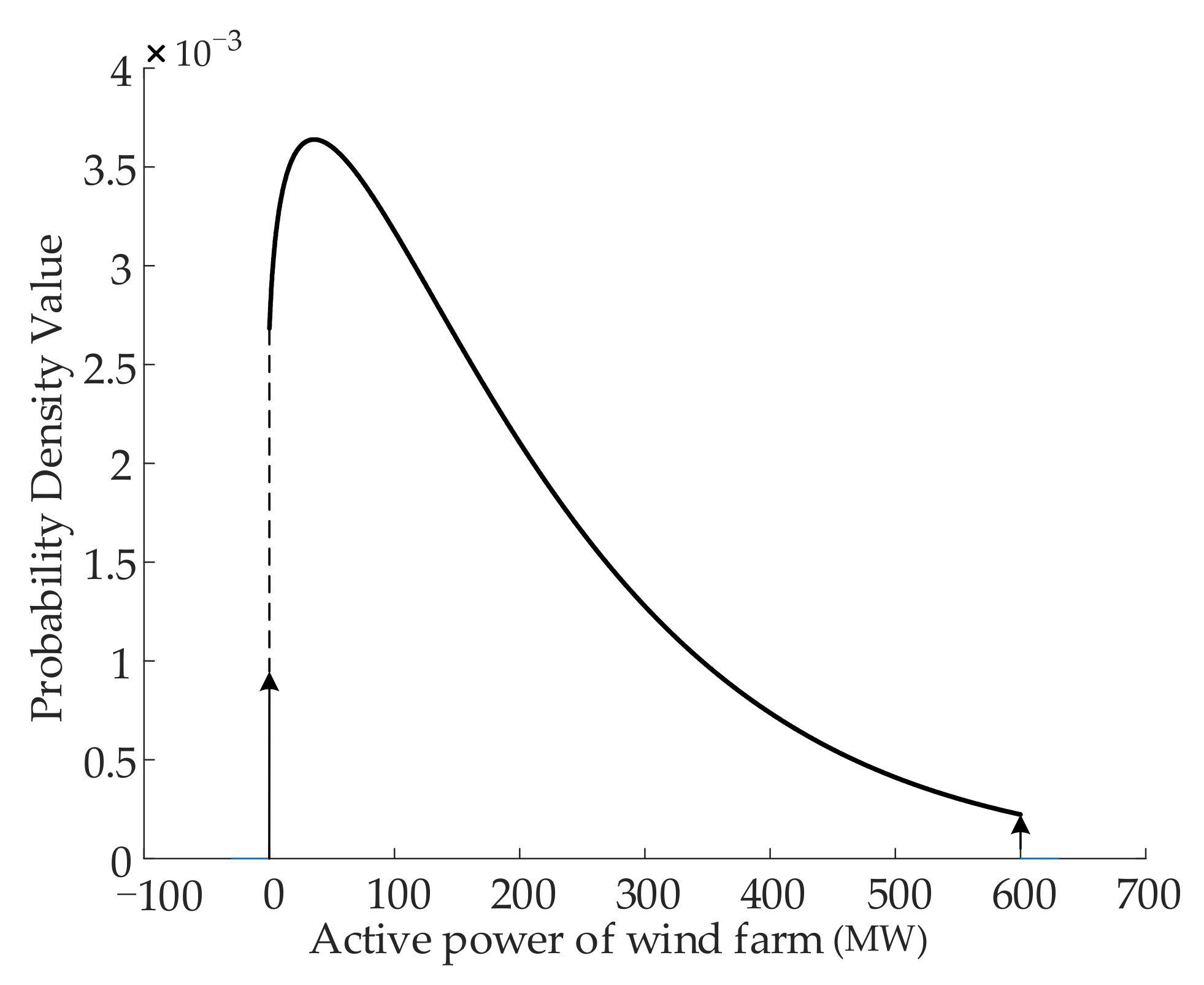
  • Based on the wake effect, we deduced the distribution characteristic model of the active power output of each wind farm by using the statistical fitting method and introducing the impulse function.
  • We considered the correlation between power shortages and curtailed wind volume and established a stochastic optimization model for WFC scheduling to improve wind power consumption capacity.
  • We improve the ADMM to decouple the model in space and time and solve the parallel iteration problem and design a power information interaction module to solve the problem of simultaneous decoupling between a large number of decision variables.
Compared with the contribution of this paper, other current research mainly has the following limitations. In [26,27], Weibull was used to fit the wind speed distribution to obtain the probability distribution of wind power, but the wake effect of the wind turbine was not considered. Papers [1,17,28] are devoted to dispatching optimization strategies for active power in wind power clusters; however, they do not consider the output characteristics of different wind farms and distributed algorithms suitable for large-scale system solving problems. Papers [18,24,29], based on ADMM, formulated an active power optimal control dispatch strategy for multiple wind farms to improve the computational efficiency of wind power dispatch problems but did not consider wind power uncertainty.
The rest of the paper is organized as follows. In Section 2 we derive the wind farm output model and describe the WFC active dispatch model. In Section 3, we derive a distributed model for ADMM application in WFC scheduling. We compare the results with previous studies in Section 4, and finally, Section 5 presents the summary and prospect for the next steps.

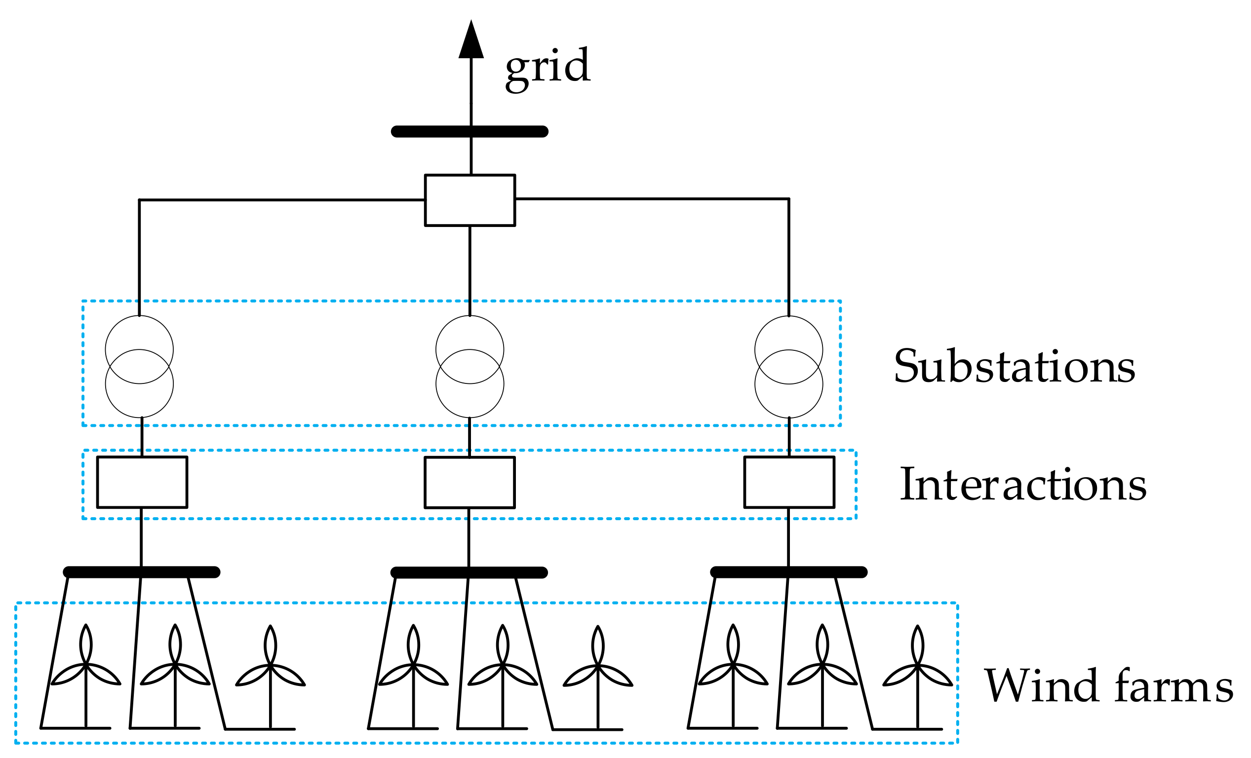
2. Active Power Dispatching Model of WFC Considering Wind Speed Uncertainty

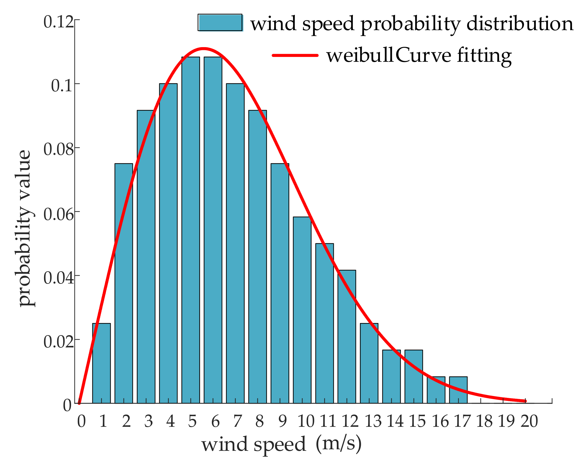
2.1. Probability Density Model of Active Power Output of Wind Farm Based on Wake Effect

We adopt the classical two-dimensional Weibull distribution to describe the wind speed probability density function [26]:
f ( v ) = k γ ( v γ ) k 1 exp [ ( v γ ) k ]
G ( v ) = P ( V v ) = 1 exp [ ( v γ ) k ]
where v is wind speed; k is shape factor; γ is scale factor; f ( v ) is probability density function; G ( v ) is cumulative probability distribution function.
We use the classical piecewise function to represent the approximate relationship between the active power output of the wind turbine and the wind speed [26]:
p = 0 , v < v in   or   v > v off v 3 v in 3 v r 3 v in 3 P r v in v v r P r v r v v off
where p is the active power of the wind turbine; P r is rated power of wind turbine; v in is the cut-in wind speed of the wind turbine; v off is cut-out wind speed; v r is rated wind speed.
The wind turbine gearbox can adopt the material process method of the decomposition strategy [30]. In addition, the conversion of the extremely low speed of the wind turbine into the extremely high speed of the generator needs to be realized by the gearbox. Most of the existing studies ignore the influence of the wake effect, assuming that the active power output of the entire wind farm is equal to the active power output of a single wind turbine multiplied by the number of wind turbines, but in fact, due to the wake effect, the wind speed of each wind turbine is not identical. We use the Jensen model to study the effect of wake effects on the active power output of wind farms, and its wind speed is shown in Equation (4) [31]:
v i = v 0 α d i 1 i = 1 , 2 , , x n α d = 1 ( 1 1 α T ) ( R R + α x d x ) 2
where v i is the wind speed obtained by the first wind turbine; α d is the proportion of wind speed drop between front and rear adjacent wind turbines; α T is thrust coefficient of the wind turbine; α x is wake attenuation coefficient; d x is the distance between the front and rear wind turbines in the wind direction.
According to the principle of the Jensen model, combined with Equations (3) and (4), the relationship between the active power output and wind speed of the wind farm can be obtained as shown in Equation (5):
p w = 0 , v < v in / α w   or   v > v off ( v     α w ) 3 v in 3 v r 3 v in 3 P wr v in / α w v v r / α w P wr v r / α w v v off
P wr = x n y n P r
α w = i = 1 x n α d i 1 / x n
where p w is the active power of wind farms; P wr is the active output of wind farms; α w is the average wake effect coefficient of wind farms; x n and y n are the number of rows and columns of the wind turbine matrix in the Jensen model. The rated power of the wind farm in Equation (6) is determined by multiplying the total number of wind turbines. We use the same row of wind turbines perpendicular to the wind direction to be equivalent to a wind turbine, and calculate the average wake effect coefficient by Equation (7). Finally, Equation (5) can be deduced by combining Equations (3) and (4).
Combining Equations (1), (2) and (5), the cumulative probability distribution function of wind farm active power can be obtained as shown in Equation (8):
H ( p w ) = G ( v in ) + 1 G ( v off ) p w = 0 1 + G ( v ) G ( v off ) 0 < p w < P wr 1 p w = P wr
It can be seen that when the output of the wind farm is equal to 0 and the rated power, the cumulative probability function curve has a step phenomenon, and the values are:
H ( 0 ) = G ( v in ) + 1 G ( v off )
H ( P wr ) = G ( v off ) G ( v r )
According to the relationship between the cumulative probability distribution function and the probability density distribution function, the probability density value is infinite when the active output of the wind farm is equal to 0 and the rated power. In order to solve this problem, this paper adopts the concept of impulse function to construct a unit impulse function δ ( P ) to represent that it tends to infinity at P = 0 . Finally, after the derivation operation, the probability density function of the active power output of the wind farm can be obtained by combining Equations (2) and (5)–(10), as shown in Equation (11):
φ ( p w ) = 0 , p w < 0 ,   p w > P wr H ( 0 ) · δ ( p w ) , p w = 0 H ( p w ) , 0 < p w < P wr H ( P wr ) · δ ( p w P wr ) , p w = P wr
where:
H ( p w ) = k ( v r 3 v in 3 ) 3 γ α w P wr [ p w P wr ( v r 3 v in 3 ) + v in 3 ] 2 3 [ 1 γ α w p w P wr ( v r 3 v in 3 ) + v in 3 3 ] k 1 exp [ ( 1 γ α w p w P wr ( v r 3 v in 3 ) + v in 3 3 ) k ]
In Equation (11), φ ( p w ) is the probability density function of active power of the wind farm composed of four-segment functions, where the independent variable is p w , and the second and fourth segment functions are impulse functions. Equation (12) is calculated by combining Equation (8) with Equations (2) and (5) through derivation. Finally, the four-piece function of Equation (11) can jointly represent the active power output probability density function curve of the wind farm.

2.2. Active Power Scheduling Model of WFC

Due to the intermittent and fluctuating wind speed, the actual output active power of the wind farm shows fluctuating characteristics during operation. Based on the dispatch instructions issued by the WFC to the wind farm, the relationship between the actual active power output of the wind farm and the dispatch instructions can be divided into three types:
  • When the actual output of the wind farm is greater than the dispatch command, it is in the “power saturation mode”, and the wind farm needs to take power curtailment measures at this time.
  • When the actual output of the wind farm is equal to the dispatch command, it is in the “power balance mode”, which is the ideal dispatch state.
  • When the actual output of the wind farm is less than the dispatch command, it is in “power shortage mode”, and the wind farm’s output is not enough to meet the dispatch command.
After the analysis of the above three situations, it is assumed that the dispatching command issued by the grid dispatching center to the WFC at a certain time is P dis , all , the maximum active power output that the wind farm can achieve under the meteorological conditions at this moment is P max , i . The method in this paper is to allocate the dispatching instructions of the WFC to each wind farm as much as possible according to the maximum active power output of the wind farm, and formulate a dispatch plan for each wind farm P dis , i to satisfy P dis , i P max , i as much as possible. Ultimately, the total output of the WFC is made to comply with the grid dispatching instructions as much as possible to reduce the grid power shortage and curtailment of wind power.

Objective Function and Constraints

Based on the predicted power probability density distribution curve of each wind farm in the WFC, and considering the probability of power shortage and curtailment of wind, the objective function is to take the expectation and minimum deviation of each wind farm’s dispatch instruction and the output probability density function as the objective function:
min t = 1 T i = 1 N E i , t E i , t = 0 P i , t , max pre p i , t P i , t pre · f ( P i , t pre ) d P i , t pre
where p i , t is the scheduling decision value; E i , t is the deviation between dispatch instruction and output probability density function; f ( x ) is the probability density function of the active power output of wind farms fitted by Weibull distribution, as shown in Equation (11); P i , t pre is the independent variables of f ( x ) .
There are the following constraints:
  • Scheduling plan value constraints:
    i = 1 N p i , t = P C , t , all dis
  • Wind farm output power limit constraints:
    P i , min p i , t P i , t , max pre P i , max
  • Substation capacity constraints:
    P tr , min p tr , i , t P tr , max
  • Transmission line capacity constraints:
    P L , max p L , i , t P L , max
  • Wind farm output power ramp constraints:
    p i , t + 1 p i , t U R i p i , t p i , t + 1 M R i
  • Wind farm regulation capacity constraints:
    p i , t > ( 1 b % ) P i , t , max pre
    where P C , t , all dis is scheduling instructions for WFC; P i , t , max pre is the wind farm forecast power cap; P i , min and P i , max are the minimum output and installed capacity of the wind farm, respectively; P tr , min and P tr , max are the minimum and maximum transmission powers of the substation, respectively; P L , max is the maximum transmission power of the line; U R i and M R i are maximum ascent rate and maximum descent rate of wind farm active output; b is the drop-out force control ratio.

3. Distributed Model for Active Power Scheduling of WFC

3.1. A Spatiotemporal Decoupling Model for Optimal Scheduling of WFC

A regional WFC is usually composed of dozens to hundreds of wind farms. The decision variables of each wind farm are coupled together by the dispatch power balance constraint shown by Equation (14). Therefore, solving the optimization scheduling problem of a WFC system with a large number of decision variables and coupled with each other brings new challenges to the control algorithm, information interaction and optimization solution methods. In the iterative convergence process of ADMM, the convergence of the penalty function term can just solve the coupling constraint problem of the WFC scheduling model and can correct this constraint. It is equivalent to integrating this constraint into the objective function of the sub-problem to achieve the purpose of decoupling each sub-optimization problem of the cluster scheduling model. To this end, we propose the following space–time decoupling optimization scheduling strategy based on ADMM.
A typical ADMM adopts a distributed serial iterative form when it iteratively converges. In order to solve the problem that each sub-optimization problem in the WFC dispatching system can be iterated in parallel, we set up an information exchange module in the adjacent wind farms and substations. Assuming that the inflow power is positive and the outflow power is negative, its structure is as follows. Figure 1. In the process of the optimization iteration of each sub-problem, adjacent wind farm modules and substation modules can exchange optimization result information in their information exchange modules to achieve the purpose of updating all global decision variables at the same time. Therefore, the corresponding spatiotemporal decoupling strategy can be described as follows. First, the scheduling instruction is equivalent to a load of the same size at the WFC grid-connected nodes. Then, the WFC dispatching system is decoupled into intelligent modules including wind farms, substations and loads, and an information exchange module; the information exchange module is responsible for the power information exchange of the entire model. Finally, all sub-optimization problems can communicate with adjacent intelligent modules only through the local sparse communication network during the update iteration process, and all the calculation processes are completed within each intelligent module.
The decoupling mode in time is performed as follows: Each intelligent module of the system performs the calculation and calculation of the active power output through the local computing chip and then sends the calculated power information to the adjacent information exchange module. The global variables, coupled variables, and Lagrange multipliers are updated and calculated on each information interaction module. According to the ADMM, the obtained results can be used to control and coordinate the direction of the global optimization, and perform automatic adjustment for the next iteration to speed up the convergence speed and improve the convergence accuracy. In the solution process, each time period is completely independent, realizing the time decoupling of control, information interaction, and optimization solution.

3.2. Distributed Optimization Algorithm Based on ADMM

According to the ADMM, the standard iterative solution form is:
x k + 1 = arg min ( f ( x ) + ( λ k ) T ( x y k ) + ρ 2 x y k 2 2 ) y k + 1 = arg min ( f ( y ) + ( λ k ) T ( y x k + 1 ) + ρ 2 y x k + 1 2 2 ) λ k + 1 = λ k + ρ ( x k + 1 y k + 1 )
where x and y are the coupling variables between modules.
It can be seen from Equation (20) that the standard ADMM is a serial iteration, and the result of another module needs to be used when the module is optimized. However, the model proposed in this paper contains optimization calculations for several sub-problems. Therefore, it is necessary to improve the standard ADMM to be suitable for the model in this paper and to be able to iteratively calculate it in parallel:
min ξ = 1 M f ξ ( p ξ )
z g k + 1 = 1 N g g G ( p ξ k + 1 )
The objective function of all sub-optimization problems can be expressed as (21), where p ξ is the coupling variable of all sub-problems. The vector average value of the coupling variable results of adjacent intelligent modules is shown in Equation (22), which is used to exchange the information of the power optimization results of each sub-problem to achieve the goal of the parallel iterative optimization of each sub-problem. Taking the first formula of Equation (20) as an example to improve, the last two terms can be expressed as:
( λ k ) T ( x y k ) + ρ 2 x y k 2 2 = ( λ k ) T x ( λ k ) T y k + ρ 2 ( x ) 2 ρ x y k + ρ 2 ( y k ) 2 = ρ 2 x y k + ( λ k ) T ρ 2 2 ( λ k ) T 2 2 2 ρ
Assume u = λ ρ and omit the constant term ( λ k ) T 2 2 2 ρ . After the improvement, the ADMM parallel iterative solution form suitable for the model in this paper is:
P ξ k + 1 = arg min ( f ξ ( p ξ ) + ρ 2 p ξ ( p ξ k z ξ k ) + u ξ k 2 2 )
z g k + 1 = ( 1 / N g ) g = 1 N g p ξ k + 1
u g k + 1 = u g k z g k + 1
where z ξ is a global variable, representing the unbalanced power vector on the information exchange module; N g is the number of dual variables that interact with global variables; p k z k represents the correction amount of the penalty function in the iterative process, and replaces the term in Equation (23). The sub-problem optimization model of Equation (24) for various intelligent modules is shown in Equations (27)–(29).
For wind farms ξ = 1 , 2 , , W , solving Equations (24)–(26) in the optimal scheduling model can be equivalent to solving the model as shown in Equation (27):
min P ξ , t t = 1 T { [ 0 P ξ , t , max p ξ , t P ξ , t pre · f ( P ξ , t pre ) d P ξ , t pre ] + ρ 2 ( p ξ , t + z ξ , t k + u ξ , t k p ξ , t k ) 2 } s . t . P ξ , min p ξ , t P ξ , t , max t = 1 , 2 , , T p ξ , t + 1 p ξ , t U R ξ t = 1 , 2 , , T p ξ , t p ξ , t + 1 M R ξ t = 1 , 2 , , T p ξ , t > ( 1 b % ) P ξ , t , max t = 1 , 2 , , T
For substations ξ = 1 , 2 , , G , solving Equations (24)–(26) in the sub-optimization model can be represented by model Equation (28):
min P ξ , t ρ 2 t = 1 T ( p ξ , t + z ξ , t k + u ξ , t k p ξ , t k ) 2 s . t . P ξ , min p ξ , t P ξ , max t = 1 , 2 , , T
For loads ξ = 1 , 2 , , D , solving Equations (24)–(26) can be equivalent to solving the sub-optimization model Equation (29):
min P ξ , t ρ 2 t = 1 T ( p ξ , t + z ξ , t k + u ξ , t k p ξ , t k ) 2 s . t . p ξ , t = D t t = 1 , 2 , , T

3.3. Model Solving

The sub-optimization problems of each module are updated iteratively in parallel according to Equations (27)–(29), until all sub-optimization problems satisfy the convergence conditions of Equation (30):
r k + 1 = z g k + 1 2 ε pri s k + 1 = ρ ( z g k z g k + 1 ) 2 ε dual
Equation (30) indicates that the original residual r and the dual residual s are less than the convergence accuracy thresholds ε pri and ε dual . The original residual is expressed as the unbalanced power on the information exchange module, and the smaller the value is, the closer the optimization results on all intelligent modules are to the optimal solution. When all the sub-optimization systems obtain the optimal solution, the whole WFC scheduling problem also obtains the global optimal solution. The dual residual is the difference between the global variables in two adjacent iterations. When the difference is smaller, the convergence of the two iterations is smaller, and it is closer to the global optimization result.
The main steps of the iterative calculation process of the ADMM used in this paper are as follows:
Step 1: Enter the cluster dispatch plan, relevant parameters and forecast information of each wind farm;
Step 2: Set k = 0, convergence accuracy and initialize power information of each module;
Step 3: The sub-problems of each intelligent module are solved in parallel according to Equation (24), and the active power results of each module are obtained;
Step 4: The active power results are transmitted to the connected information exchange module;
Step 5: The information exchange module collects the power information transmitted by the connected intelligent modules and updates and calculates according to Equations (25) and (26);
Step 6: The information interaction module sends the calculation result of step (3) to its connected intelligent module and enters the next iteration. Until ADMM converges and the global optimal solution is obtained, the cycle ends.

4. Case Analysis

This paper uses the relevant wind speed data and actual output data from eight wind farms in a WFC base in Northwest China. The actual measured value and predicted upper limit of wind speed and active power output in September 2017, with a sampling interval of 15 min. We use wind speed data and forecast data to build a model, and use the measured value of active power output to analyze and verify the effectiveness of the method proposed in this paper. Among them, the installed capacity of eight wind farms in the cluster is shown in Table 1.
The values of the relevant parameters in the example system are as follows: cut-in wind speed v in is 3.5 m/s; cut out wind speed v off is 15 m/s; rated wind speed v r is 10.5 m/s; the control ratio of the wind farm’s output reduction b is 0.8; the Lagrangian parameter ρ is 4.0.

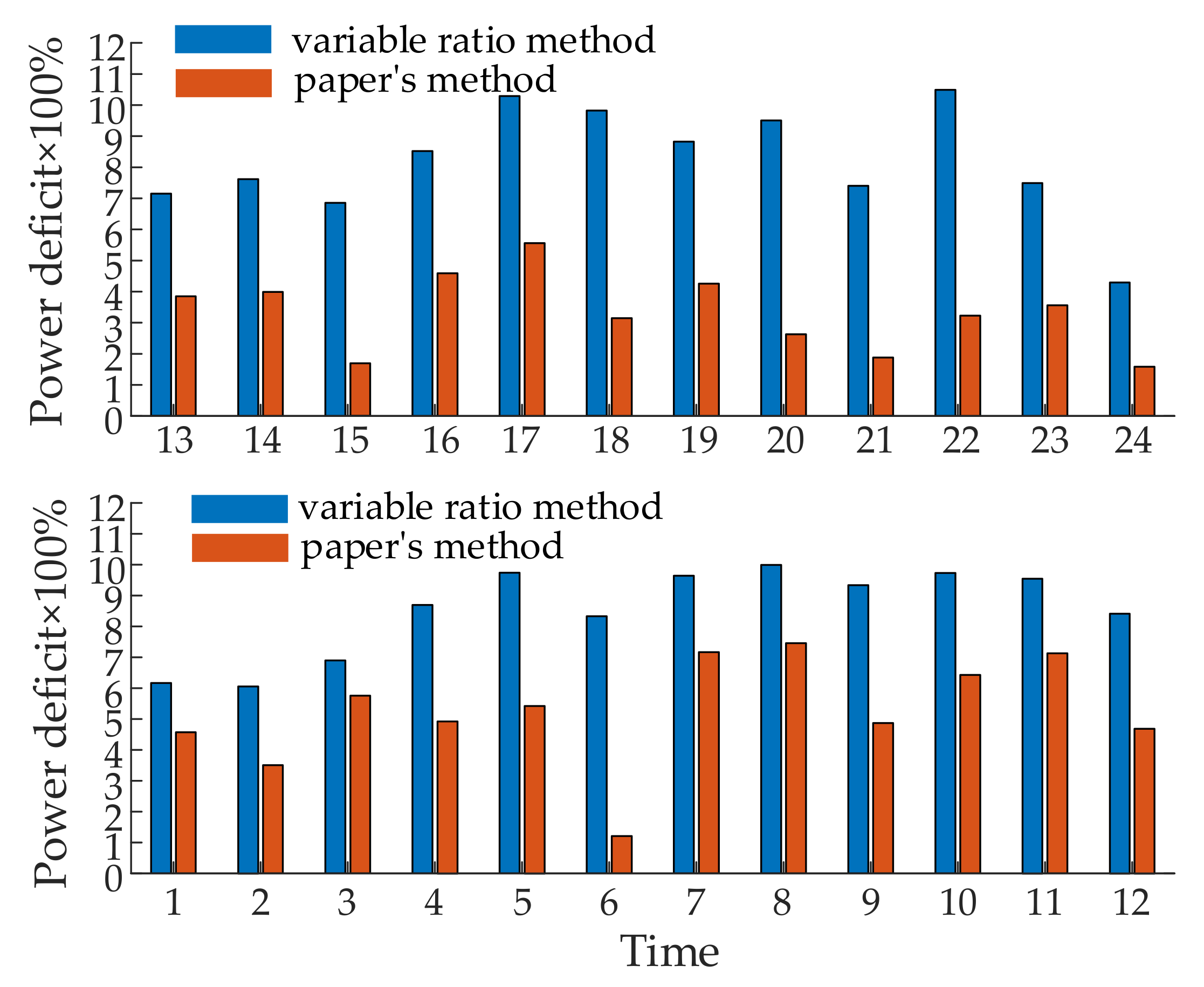
4.1. Optimization Results and Analysis

The Weibull fitting curve of wind speed in the first period of the wind farm WF1 is shown in Figure 2, and the probability density curve of active power output is shown in Figure 3. It can be seen from Figure 2 that the curve obtained by the Weibull fitting algorithm can very accurately fit the distribution characteristics of wind speed, indicating that the probability distribution of wind power output obtained by this method is very close to the actual situation. It can be seen from Figure 3 that the output probability value of the wind farm changes with the probability of wind speed, and the curve is very smooth, indicating that the wind farm active power output probability density curve obtained by considering the wake effect can actually describe the wind speed uncertainty, making the scheduling method in this paper more practical.
The active power distribution method of WFC is to allocate active power dispatching instructions to each wind farm in proportion according to the installed capacity of wind farms to achieve the purpose of fair distribution. The calculation formula is shown in Equation (31), and Equations (32) and (33) are used to calculate the power shortage generated by the WFC and the wind power utilization rate of each wind farm using the method in this paper and the variable-ratio method, respectively:
P dis , n ( t ) = P N , n P N , all P dis , all ( t )
η = P dis , all P real P real × 100 %
λ = P real P real , max P real , max × 100 %
where P dis , n ( t ) is scheduling plans for wind farms; P N , n , P N , all are the installed capacity of wind farms and WFC; P dis , all ( t ) is the general dispatch command issued by the grid dispatch center to the WFC; P real is the total actual output of the WFC; P real , m a x is the actual maximum output power of the wind farm.
It can be seen from Figure 4 that, compared with the variable-proportion allocation algorithm, the dispatching power shortage caused by the optimal dispatching of the WFC using the method in this paper can be greatly reduced. It shows that the dispatch plan obtained by the method in this paper is closer to the actual active power output of the WFC and has a very high confidence level. As can be seen from Figure 5, for each wind farm within the WFC, when the optimization algorithm in this paper is used to formulate the WFC dispatch plan, the wind power utilization rate of each wind farm is improved significantly compared with the variable proportion allocation algorithm. This is because wind power is intermittent and fluctuating, and the dispatch plan formulated according to the traditional variable-ratio method cannot meet the actual wind power output. However, the method in this paper considers the wake effect of the wind turbine and the distribution characteristics of the active power output of each wind farm, so that the WFC scheduling is more practical.

4.2. ADMM Testing and Analysis

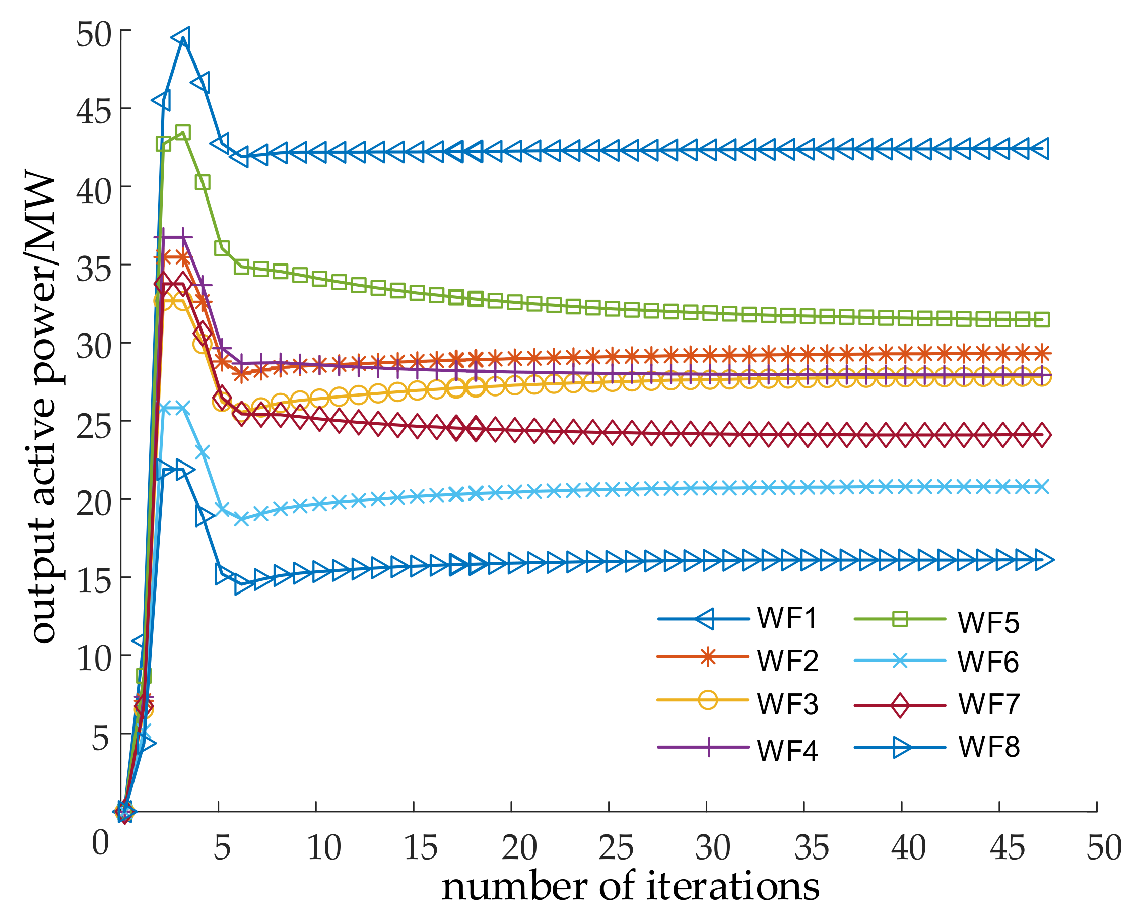
4.2.1. Effectiveness Test

The ADMM and the direct solution method are used to calculate the WFC system model. The output results of each wind farm are obtained, and the results of the first period are compared, as shown in Table 2. It can be seen that the output results of each wind farm under the direct solution method and the distributed algorithm basically coincide. After calculation, the maximum deviation rate is 4.398 × 10⁻³ (deviation rate = deviation value/installed capacity of wind farm). The results verify the effectiveness and correctness of the algorithm in this paper.

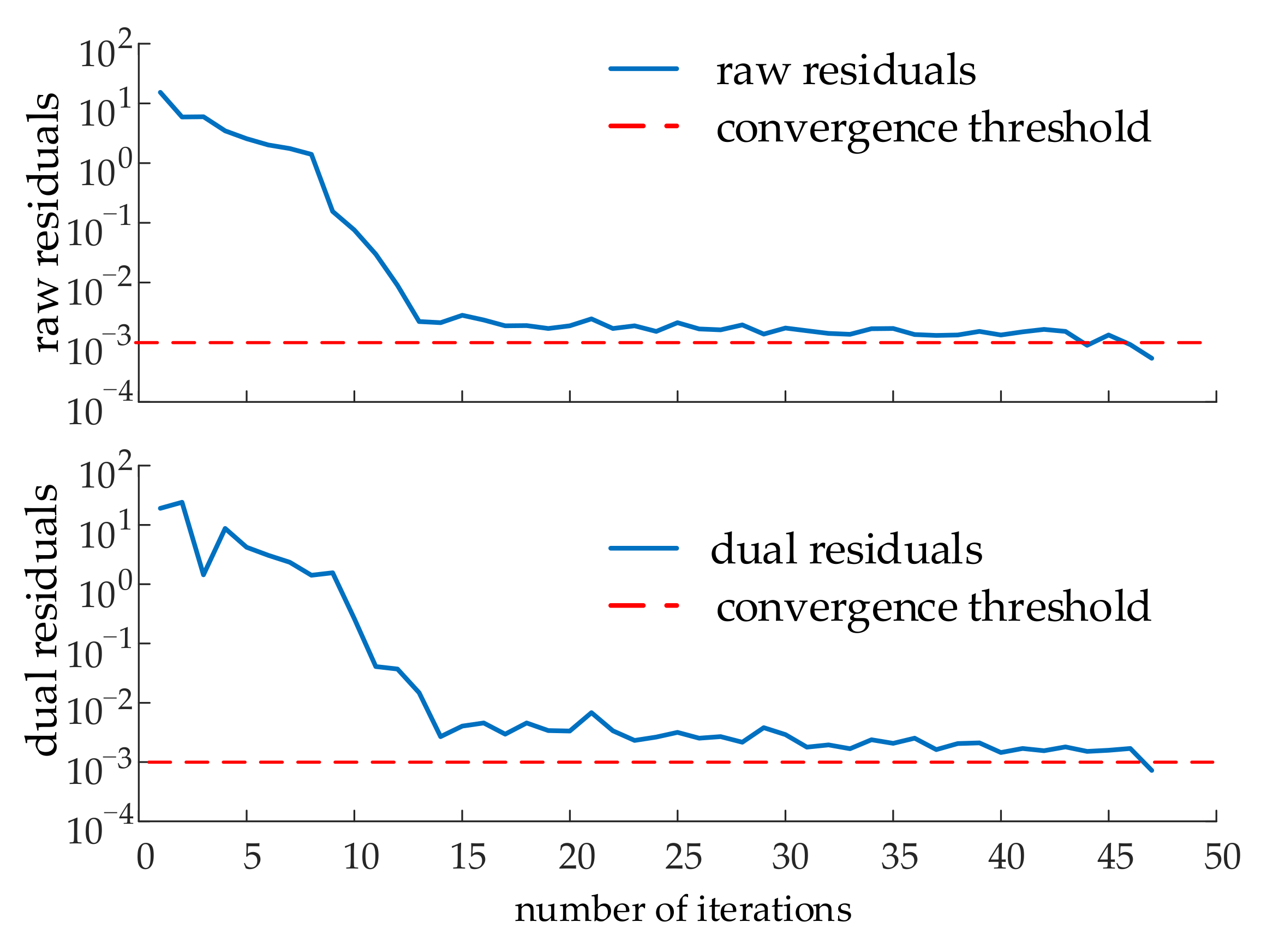
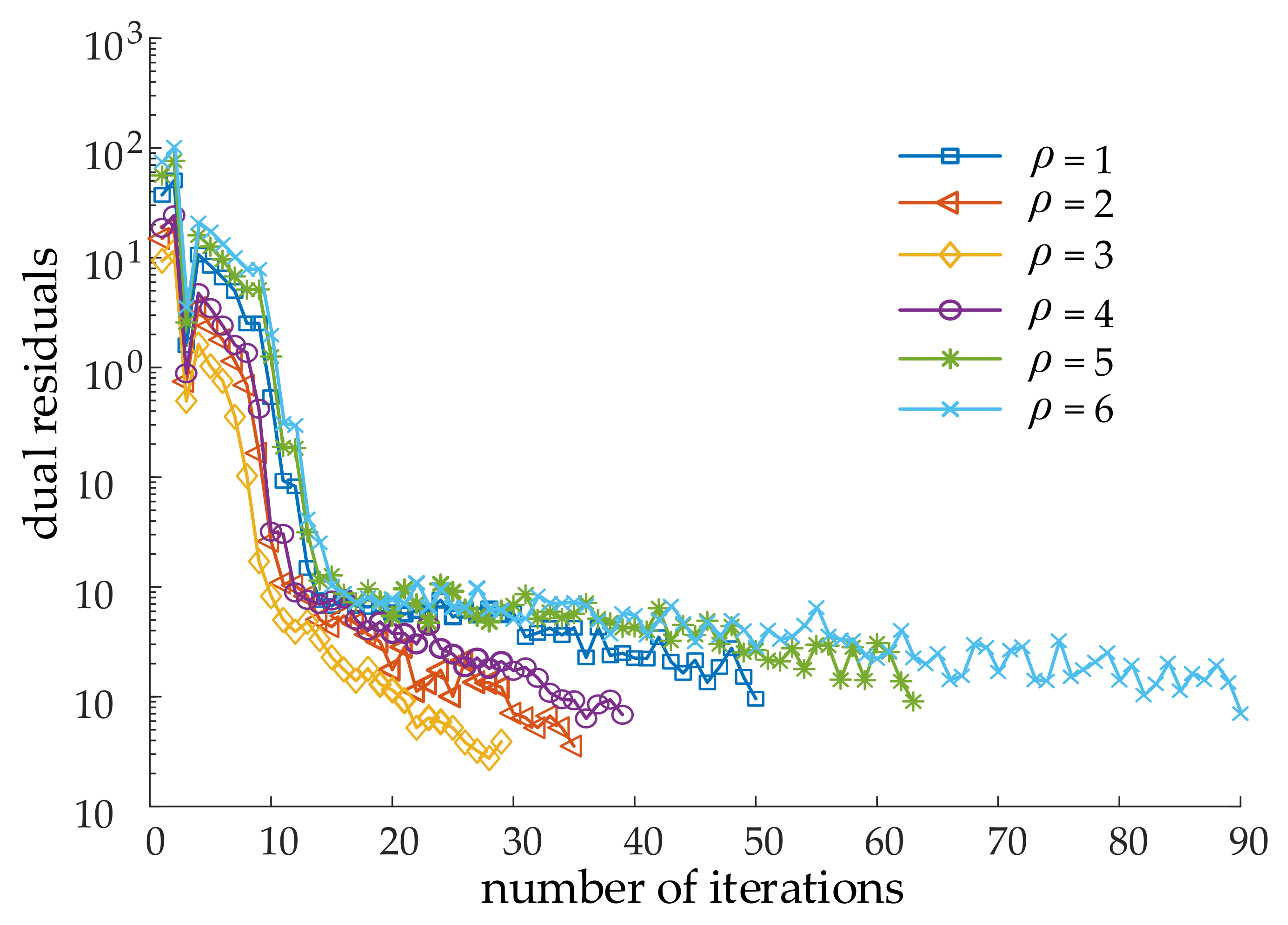
4.2.2. Convergence Test

Figure 6 and Figure 7 are the convergence curve of the original residual, the dual residual and the active power output of each wind farm obtained by applying the ADMM. It can be seen that the convergence curves of the original residual and the dual residual both show a downward trend, the first half of the decline speed is faster, the second half of the decline speed tends to be flat, and finally, both can converge to 0 within a limited number of iterations, which can reach the preset convergence threshold. The active power output iteration result curves of each wind farm can reach convergence, and each curve can smoothly and stably converge to the optimal value at the later stage of iteration. It shows that the sub-problems of this algorithm can be distributed computing, and the whole big problem can be converged to obtain the optimal solution when all the sub-problems are converged by finite iterative coordination. The algorithm has strong stability.
The convergence speed of the ADMM is mainly affected by the Lagrangian update step size ρ . Figure 8 shows the relationship between the algorithm convergence speed and the update step size for the eight wind farms system. It can be seen that the value of ρ has a great influence on the convergence speed of the system. When three is selected, the convergence is the fastest, and six is the slowest convergence. After a large number of tests, WFC systems of various scales can converge when ρ is one to six, indicating that a suitable value can be found through multiple trials to make the system achieve a faster convergence speed. Therefore, in the application of the actual system, the relative optimal value of the update step size ρ can be realized through a certain number of experiments.

4.2.3. Efficiency Test

We constructed wind farms WF1, WF2 and WF3 into a local WFC and constructed two WFC systems with 12 and 16 wind farms, respectively. The calculation time obtained according to centralized dispatch and distributed dispatch is shown in Table 3.
It can be seen that the computing time of a single sub-problem in each iteration of distributed computing is the solution time for the entire system to complete the iteration. For WFC systems with different numbers of wind farms, the average iteration time of sub-problems solved by ADMM will not change significantly. As the number of wind farms increases, the distributed computing time is only related to the number of iterations, while the centralized solution time tends to increase geometrically. This is because large-scale systems have the problem of dimensionality disaster in the centralized optimization solution. The distributed algorithm can decompose the entire system into several modular units and solve them independently in parallel. Regardless of the size of the system, the sub-problem-solving complexity of the ADMM is basically unchanged. It just solves the problem of dimensionality disaster in the optimal scheduling of large-scale WFC systems. Therefore, when the scale of the WFC system reaches a certain level, the computing time of the centralized algorithm shows a geometric trend with the increase in the system scale, and the ADMM has incomparable advantages.

5. Conclusions

Aiming at the problems of the low utilization rate of wind power caused by wind power uncertainty and dimensional disaster caused by the centralized grid connection of large-scale wind power, a distributed active power dispatching method for WFC considers the distribution characteristics of the active power output of wind farms is proposed. By solving the model, the following conclusions are obtained:
(1)
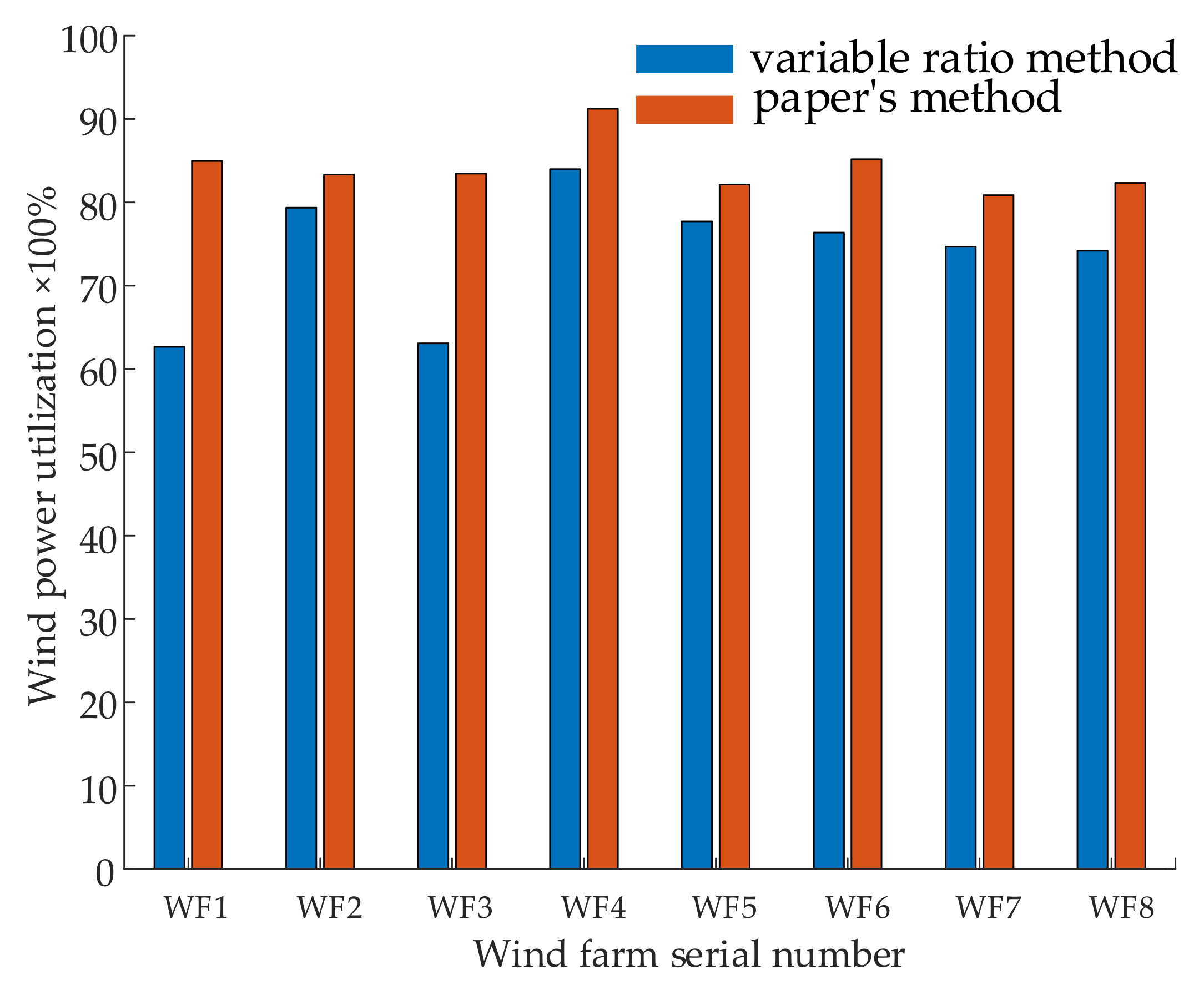
The active power output probability density characteristic model of wind farms considering the uncertainty of wind power can reduce the power shortage of wind power dispatching and improve the utilization rate of wind power. The results show that the model has a 3–7% reduction in dispatched power shortfalls and a 4–21% improvement in wind power utilization. It shows that under the influence of wind power uncertainty, considering the probability density characteristics of wind power is also an effective method to improve the utilization rate of wind power.
(2)
When solving a large-scale WFC scheduling model with the disaster of dimensionality problem, when the number of wind farms is greater than eight, the distributed dispatching method based on ADMM has extremely high computational efficiency. When the update step size is taken to an appropriate value, it has good convergence characteristics and has better advantages than centralized dispatching.
(3)
The active power distributed dispatching method of WFC proposed in this paper can not only meet the needs of parallel solution of each module unit, but also improve the ability of large-scale wind power to participate in grid dispatching.

Author Contributions

Conceptualization, P.H. and Z.Q.; methodology, P.H.; software, P.H.; validation, P.H.; formal analysis, P.H.; investigation, P.H.; resources, Z.Q.; data curation, P.H.; writing—original draft preparation, P.H.; writing—review and editing, Z.Q.; visualization, Z.Q.; supervision, Z.Q.; project administration, Z.Q.; funding acquisition, Z.Q. All authors have read and agreed to the published version of the manuscript.

Funding

This research was funded by the Guangxi Natural Science Foundation of China, grant number 2021GXNSFAA220042 and the National Natural Science Foundation of China, grant number 51767001.

Institutional Review Board Statement

Not applicable.

Informed Consent Statement

Not applicable.

Data Availability Statement

This study did not report any data.

Conflicts of Interest

The authors declare no conflict of interest.

References

  1. Jadidi, S.; Badihi, H.; Zhang, Y. Fault-Tolerant Cooperative Control of Large-Scale Wind Farms and Wind Farm Clusters. Energies 2021, 14, 7436. [Google Scholar] [CrossRef]
  2. Padinharu, D.K.K.; Li, G.J.; Zhu, Z.Q.; Clark, R.; Thomas, A.; Azar, Z.; Duke, A. Permanent Magnet Vernier Machines for Direct-Drive Offshore Wind Power: Benefits and Challenges. IEEE Access 2022, 10, 20652–20668. [Google Scholar] [CrossRef]
  3. Vali, M.; Petrović, V.; Pao, L.Y.; Kühn, M. Model Predictive Active Power Control for Optimal Structural Load Equalization in Waked Wind Farms. IEEE Trans. Control. Syst. Technol. 2022, 30, 30–44. [Google Scholar] [CrossRef]
  4. Liu, Y.; Qiao, Y.; Han, S.; Xu, Y.; Geng, T.; Ma, T. Quantitative Evaluation Methods of Cluster Wind Power Output Volatility and Source-Load Timing Matching in Regional Power Grid. Energies 2021, 14, 5214. [Google Scholar] [CrossRef]
  5. Qiao, Y.; Liu, Y.; Chen, Y.; Han, S.; Wang, L. Power Generation Performance Indicators of Wind Farms Including the Influence of Wind Energy Resource Differences. Energies 2022, 15, 1797. [Google Scholar] [CrossRef]
  6. Shi, J.; Liu, Y.; Li, Y.; Liu, Y.; Roux, G.; Shi, L.; Fan, X. Wind Speed Forecasts of a Mesoscale Ensemble for Large-Scale Wind Farms in Northern China: Downscaling Effect of Global Model Forecasts. Energies 2022, 15, 896. [Google Scholar] [CrossRef]
  7. Zhang, N.; Kang, C.; Xia, Q.; Liang, J. Modeling conditional forecast error for wind power in generation scheduling. IEEE Trans. Power Syst. 2013, 29, 1316–1324. [Google Scholar] [CrossRef]
  8. Zhang, Z.; Sun, Y.; Gao, D.W.; Lin, J.; Cheng, L. A Versatile Probability Distribution Model for Wind Power Forecast Errors and Its Application in Economic Dispatch. IEEE Trans. Power Syst. 2013, 28, 3114–3125. [Google Scholar] [CrossRef]
  9. Lorca, A.; Sun, X.A. Adaptive Robust Optimization With Dynamic Uncertainty Sets for Multi-Period Economic Dispatch Under Significant Wind. IEEE Trans. Power Syst. 2015, 30, 1702–1713. [Google Scholar] [CrossRef] [Green Version]
  10. Zhou, Y.; Zhai, Q.; Zhou, M.; Li, X. Generation Scheduling of Self-Generation Power Plant in Enterprise Microgrid With Wind Power and Gateway Power Bound Limits. IEEE Trans. Sustain. Energy 2020, 11, 758–770. [Google Scholar] [CrossRef]
  11. Ebrahimi, F.M.; Khayatiyan, A.; Farjah, E. A novel optimizing power control strategy for centralized wind farm control system. Renew. Energy 2016, 86, 399–408. [Google Scholar] [CrossRef]
  12. Lu, Z.; Ye, X.; Qiao, Y.; Min, Y. Initial exploration of wind farm cluster hierarchical coordinated dispatch based on virtual power generator concept. CSEE J. Power Energy Syst. 2015, 1, 62–67. [Google Scholar] [CrossRef]
  13. Jayasekara, S.; Halgamuge, S.K.; Attalage, R.A.; Rajarathne, R. Optimum sizing and tracking of combined cooling heating and power systems for bulk energy consumers. Appl. Energy 2014, 118, 124–134. [Google Scholar] [CrossRef]
  14. Lu, M.; Chang, C.; Lee, W.; Wang, L. Combining the Wind Power Generation System With Energy Storage Equipment. IEEE Trans. Ind. Appl. 2009, 45, 2109–2115. [Google Scholar]
  15. Han, L.; Romero, C.E.; Wang, X.; Shi, L. Economic dispatch considering the wind power forecast error. IET Gener. Transm. Distrib. 2018, 12, 2861–2870. [Google Scholar] [CrossRef]
  16. Lu, X.; Chan, K.W.; Xia, S.; Zhou, B.; Luo, X. Security-Constrained Multiperiod Economic Dispatch With Renewable Energy Utilizing Distributionally Robust Optimization. IEEE Trans. Sustain. Energy 2019, 10, 768–779. [Google Scholar] [CrossRef]
  17. Tang, C.; Xu, J.; Sun, Y.; Liu, J.; Li, X.; Ke, D.; Yang, J.; Peng, X. A Versatile Mixture Distribution and Its Application in Economic Dispatch with Multiple Wind Farms. IEEE Trans. Sustain. Energy 2017, 8, 1747–1762. [Google Scholar] [CrossRef]
  18. Huang, S.; Gong, Y.; Wu, Q.; Rong, F. Two-tier combined active and reactive power controls for VSC–HVDC-connected large-scale wind farm cluster based on ADMM. IET Renew. Power Gener. 2020, 14, 1379–1386. [Google Scholar] [CrossRef]
  19. Fang, X.; Hodge, B.-M.; Jiang, H.; Zhang, Y. Decentralized wind uncertainty management: Alternating direction method of multipliers based distributionally-robust chance constrained optimal power flow. Appl. Energy 2019, 239, 938–947. [Google Scholar] [CrossRef]
  20. He, X.; Zhao, Y.; Huang, T. Optimizing the Dynamic Economic Dispatch Problem by the Distributed Consensus-Based ADMM Approach. IEEE Trans. Ind. Inform. 2020, 16, 3210–3221. [Google Scholar] [CrossRef]
  21. Liu, W.-J.; Chi, M.; Liu, Z.-W.; Guan, Z.-H.; Chen, J.; Xiao, J.-W. Distributed optimal active power dispatch with energy storage units and power flow limits in smart grids. Int. J. Electr. Power Energy Syst. 2019, 105, 420–428. [Google Scholar] [CrossRef]
  22. Zhang, X.; Gao, B.; Zhong, J. Decentralized Economic Dispatching of Multi-Micro Grid Considering Wind Power and Photovoltaic Output Uncertainty. IEEE Access 2021, 9, 104093–104103. [Google Scholar]
  23. Huang, S.; Wu, Q.; Guo, Y.; Chen, X.; Zhou, B.; Li, C. Distributed Voltage Control Based on ADMM for Large-Scale Wind Farm Cluster Connected to VSC-HVDC. IEEE Trans. Sustain. Energy 2020, 11, 584–594. [Google Scholar] [CrossRef]
  24. Huang, S.; Wu, Q.; Guo, Y.; Rong, F. Hierarchical Active Power Control of DFIG-Based Wind Farm With Distributed Energy Storage Systems Based on ADMM. IEEE Trans. Sustain. Energy 2020, 11, 1528–1538. [Google Scholar] [CrossRef]
  25. Li, P.; Yang, M.; Yu, Y.; Hao, G.; Li, M. Decentralized Distributionally Robust Coordinated Dispatch of Multiarea Power Systems Considering Voltage Security. IEEE Trans. Sustain. Energy 2021, 57, 3441–3450. [Google Scholar] [CrossRef]
  26. Liu, X.; Xu, W. Economic Load Dispatch Constrained by Wind Power Availability: A Here-and-Now Approach. IEEE Trans. Sustain. Energy 2010, 1, 2–9. [Google Scholar] [CrossRef]
  27. Yeh, T.H.; Wang, L. A Study on Generator Capacity for Wind Turbines Under Various Tower Heights and Rated Wind Speeds Using Weibull Distribution. IEEE Trans. Sustain. Energy 2008, 23, 592–602. [Google Scholar]
  28. Lin, Z.; Chen, Z.; Qu, C.; Guo, Y.; Liu, J.; Wu, Q. A hierarchical clustering-based optimization strategy for active power dispatch of large-scale wind farm. Int. J. Electr. Power Energy Syst. 2020, 121, 106155. [Google Scholar] [CrossRef]
  29. Liao, W.; Li, P.; Wu, Q.; Huang, S.; Wu, G.; Rong, F. Distributed optimal active and reactive power control for wind farms based on ADMM. Int. J. Electr. Power Energy Syst. 2021, 129, 106799. [Google Scholar] [CrossRef]
  30. Xiao, X.; Joshi, S. Process planning for five-axis support free additive manufacturing. Addit. Manuf. 2020, 36, 101569. [Google Scholar] [CrossRef]
  31. Liang, Z.; Liu, H. Layout Optimization of a Modular Floating Wind Farm Based on the Full-Field Wake Model. Energies 2022, 15, 809. [Google Scholar] [CrossRef]
Figure 1. Distributed model of WFC system.
Energies 15 02706 g001
Figure 2. Fitting effect of wind speed probability distribution.
Energies 15 02706 g002
Figure 3. Probability density curve of wind farm active power output.
Energies 15 02706 g003
Figure 4. Dispatch power shortage of paper’s method and variable proportion method in 24 periods.
Energies 15 02706 g004
Figure 5. Wind power utilization rate of two wind farms with different methods.
Energies 15 02706 g005
Figure 6. Original residual and dual residual convergence curves.
Energies 15 02706 g006
Figure 7. Active output convergence curve of each wind farm.
Energies 15 02706 g007
Figure 8. Relationship between convergence rate of dual residual and dual step size.
Energies 15 02706 g008
Table 1. Wind farm installed capacity of WFC.
Wind FarmCapacity /MWWind FarmCapacity /MW
WF 1316WF 5450
WF 2295WF 6281
WF 3265WF 7289
WF 4450WF 8230
Table 2. Comparison of centralized and distributed algorithm results.
WFSolve DirectlyADMMWFSolve DirectlyADMM
138.0037.92529.8030.10
229.7029.64619.2419.00
335.2034.99722.1022.17
430.4030.49815.3015.30
Table 3. Calculation time of different scale systems.
Number of WFAlgorithmIterationsCalculate Total Time/sMean Iteration Time/s
3centralization112.112.1
distribution36188.66.5
8centralization159.359.3
distribution47236.16.8
12centralization1243.6243.6
distribution54378.07.0
16centralization1458.9458.9
distribution61433.17.1
Publisher’s Note: MDPI stays neutral with regard to jurisdictional claims in published maps and institutional affiliations.

