
Advanced Forecasting Methods of 5-Minute Power Generation in a PV System for Microgrid Operation Control


Abstract
:1. Introduction
1.1. Related Works
1.2. Objective and Contribution
- Carry out an analysis of the statistical properties of a time series of the measured values of 5 min power generation in a PV system;
- Verify the usefulness of the available input variables—perform a validity analysis (the time series of solar irradiance, air temperature, PV module temperature, wind direction, and wind speed) using four different methods and select eight sets of input variables to make forecasts using various methods;
- Check the efficiency of 5 min horizon power-generation forecasts by means of ten forecasting methods, including machine learning, hybrid, and ensemble methods (several hundred various models with different set values of parameters/hyperparameters have been verified for this purpose);
- Point out forecasting methods that are the most effective for this 5 min power-generation time series depending on the number of input variables used.
- The selected contributions of this paper are as follows:
- The research concerns unique data—a time series of 5 min power-generation values in a small, consumer PV system. In the case of such small PV systems and such a short forecast horizon (5 min), meteorological forecasts are usually not used in the forecasting process due to difficulties in obtaining them, which makes it problematic to obtain forecasts with very high accuracy;
- We provide a detailed description of the performance of photovoltaic systems regarding the main environmental parameters;
- We performed extensive statistical analyses of the available time series (including an analysis of the importance of the input variables);
- We used tests of ten different prognostic methods (including hybrid and team methods);
- We developed a new, proprietary forecasting method—a hybrid method using three independent, MLP-type neural networks;
- We indicate the most favorable prognostic methods for various sets of input variables (from 3 input variables to 15 input variables) and formulate practical conclusions regarding the problem under study, e.g., from the point of view of microgrids’ operation.
- We provide a broad comparative analysis of forecasting methods of a very-short-term horizon for power generation in PV systems that can be connected to low-voltage microgrids.
2. Performance of Photovoltaic Systems
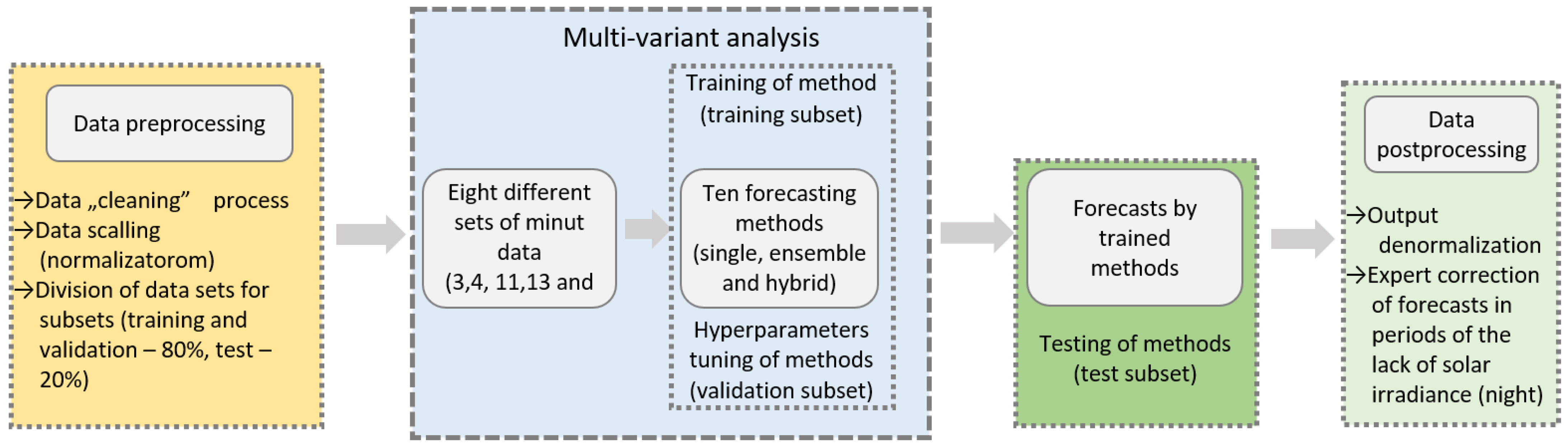
3. Data
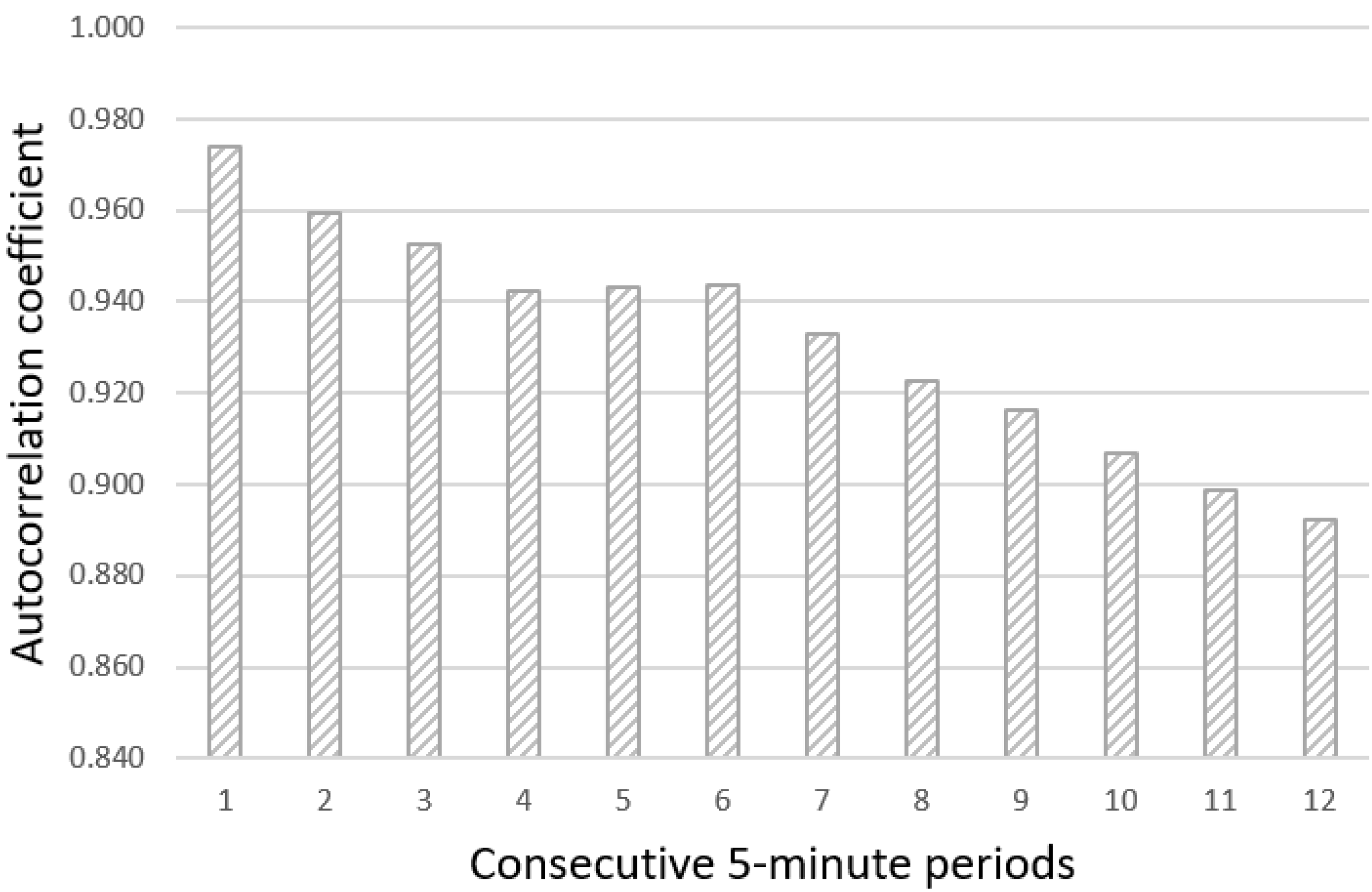
3.1. Statistical Analysis of the Time Series of Power-Generation Data
3.2. Analysis of Potential Input Data for Forecasting Methods
- Solar irradiance (W/m2);
- Air temperature (°C);
- PV module temperature (°C);
- Wind direction (degrees);
- Wind speed (m/s).
- C&RT decision trees algorithm for the selection of variables in regression problems—for each potential predictor (input data), the coefficient of determination R2 is calculated;
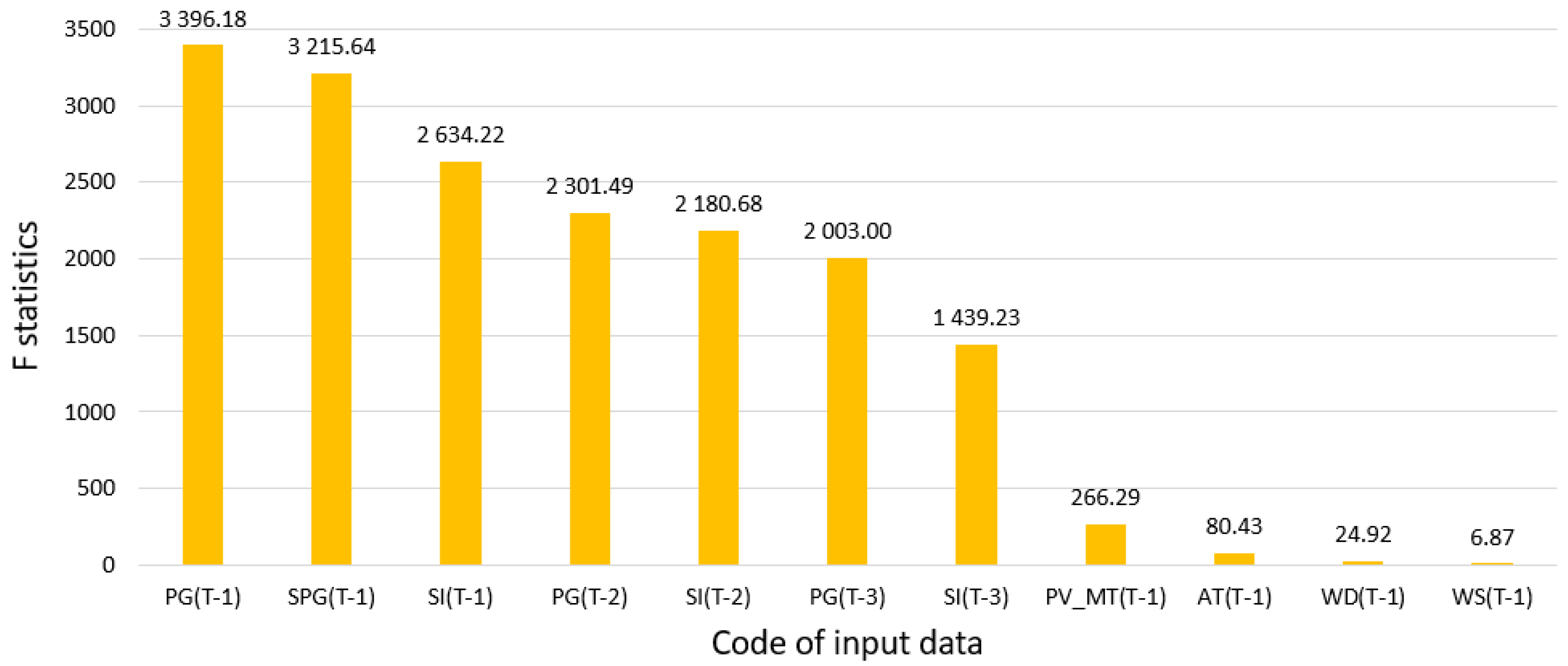
- Analysis of variances (F statistics)—this method calculates the quotient of the intergroup variance to the intragroup variance (the dependent variable) in predictor intervals (the number of quantitative predictor classes is determined before the analysis);
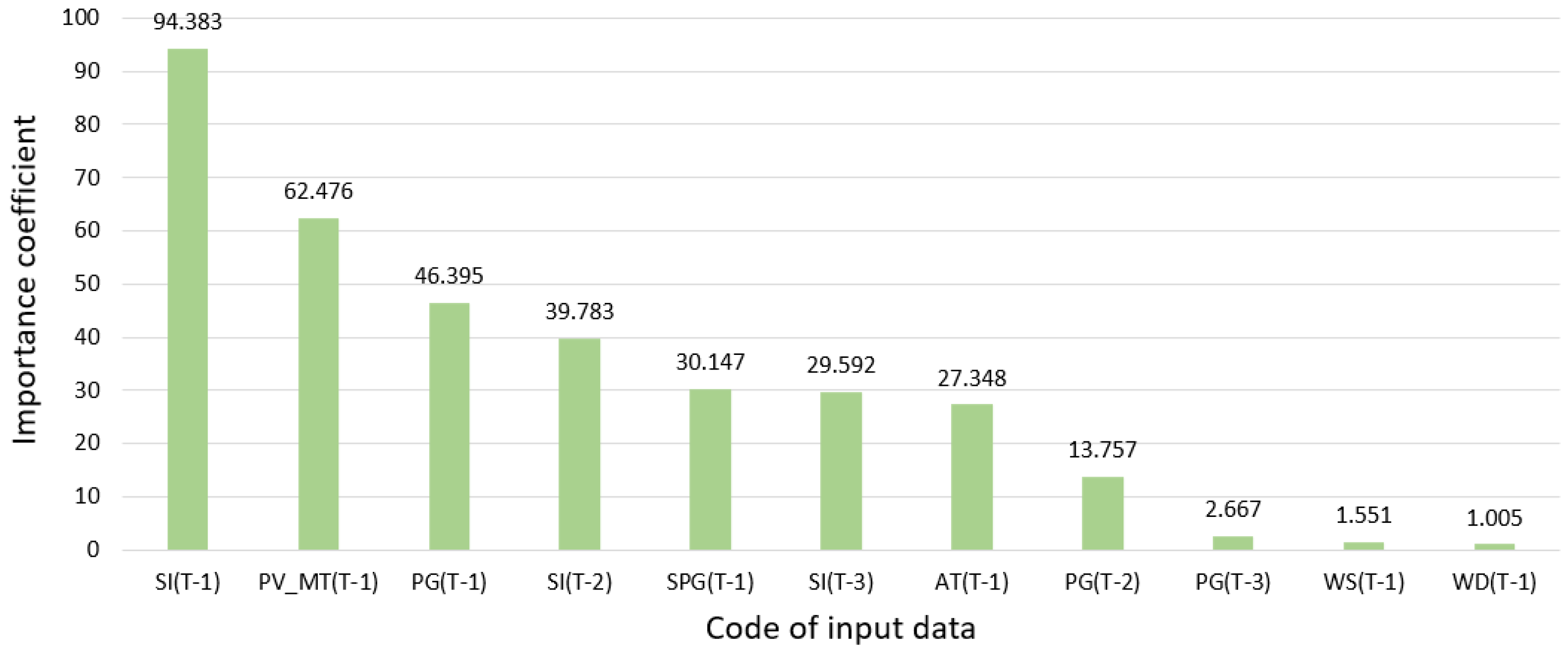
- Global Sensitivity Analysis (GSA statistics) for multilayer perceptron (MLP) neural network. A neural network with one hidden layer and four neurons in this layer was used for the analysis. The training algorithm is BFGS, the activation function in the hidden layer is the hyperbolic tangent, and the activation function in the output layer is linear. The value of the importance factor for input data number k is the quotient of the RMSE error of the forecasts of the trained MLP network using the remaining 10 input data and the input data number k is replaced by its mean value from the total data to the RMSE error of the forecasts using all 11 sets of input data. The greater the value of the importance factor for the given input data, the greater their significance. Results below 1 for a given input data mean that these input data can probably be eliminated because the MLP network without these input data has a lower RMSE error in the forecasts;
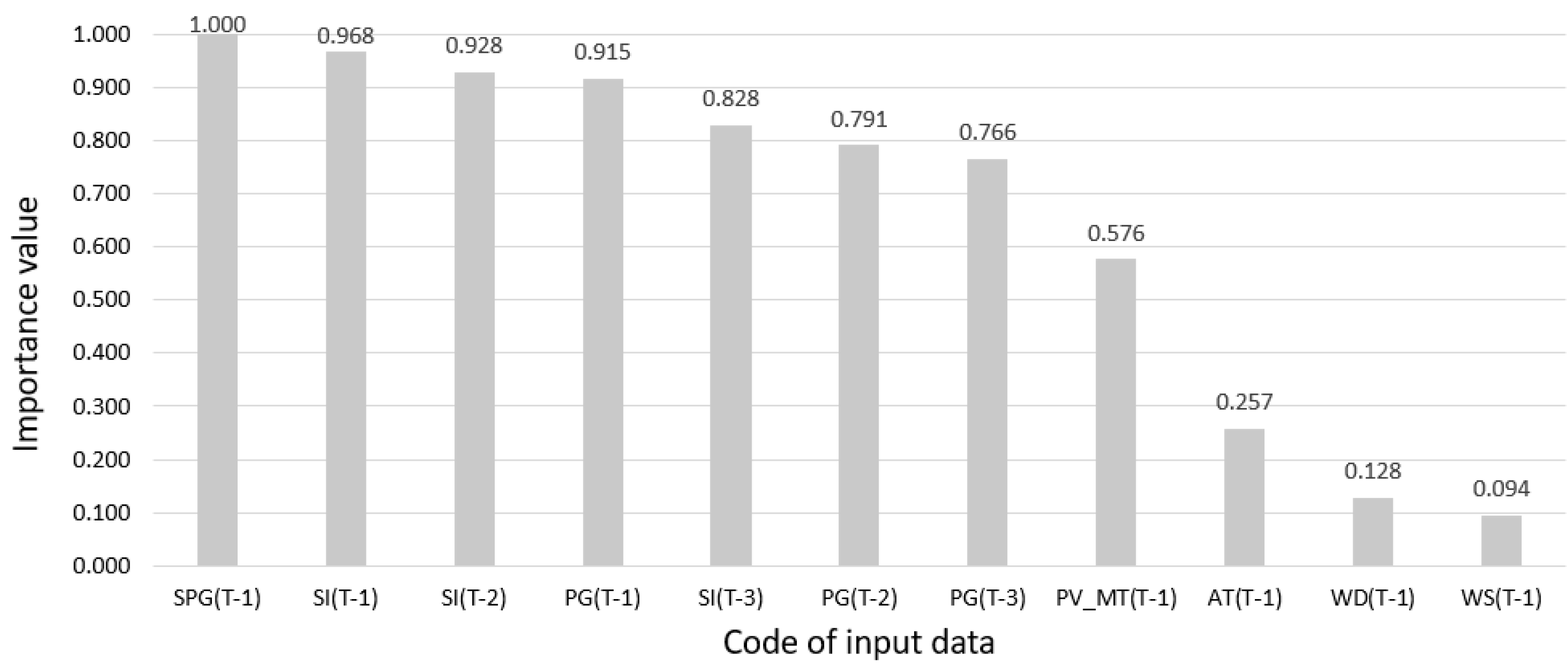
- The importance of input data using the random forest (RF) algorithm is the many decision trees (DCs). The importance of the given input data is measured by checking to what extent nodes (in all decision trees) using the input data reduce the impurity Gini indicator, with the weight of each node being equal to the number of associated training samples [38]. It was assumed for the analysis that each decision tree would have 6 randomly selected sets of input data from the total of 11.
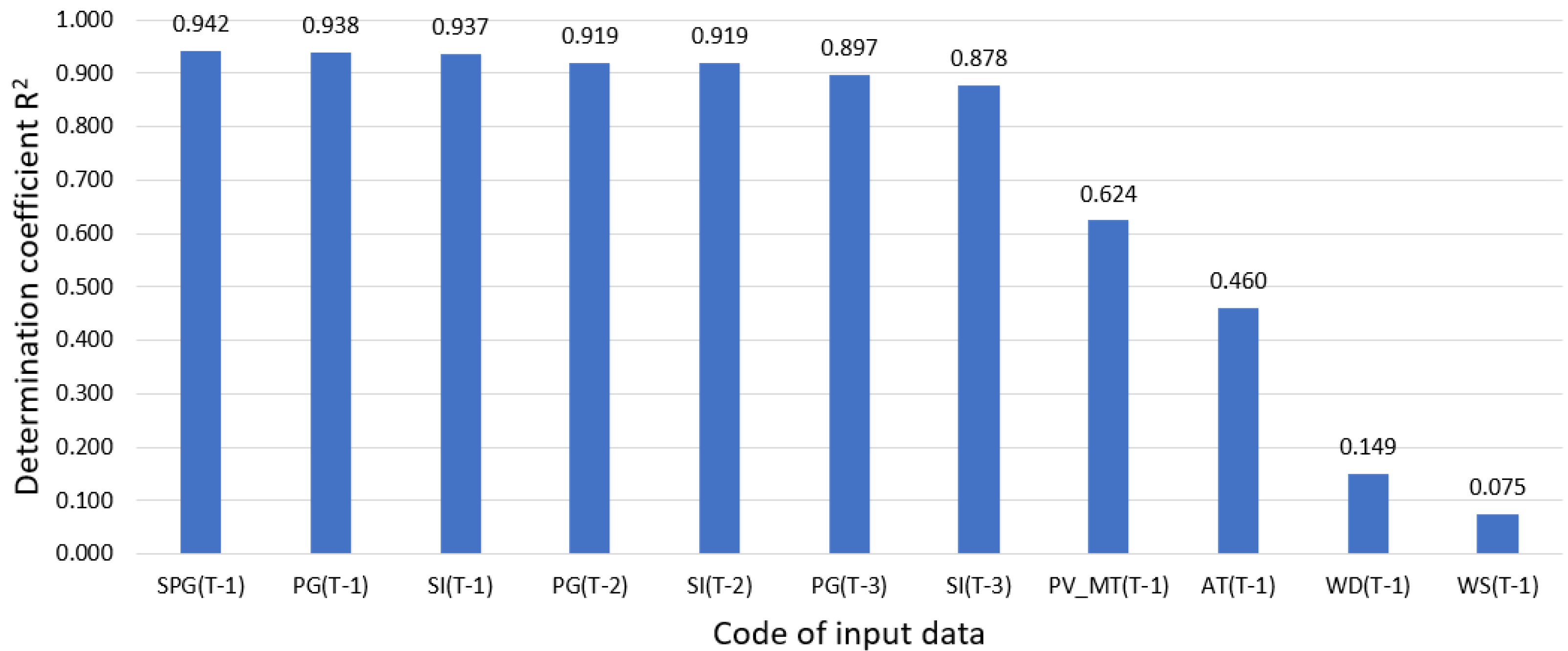
- For all analyzed methods of selecting variables, the significantly least important input data are wind direction in period t−1 and wind speed in period t−1. In the vast majority of cases, the last, least-important input data are (somewhat surprisingly) wind speed in period t−1;
- The best input data include smoothed power generation in period t−1, power generation in period t−1, and solar irradiance in period t−1.
- The results of the individual selection methods were quite similar, except for the input-data-selection method using global sensitivity analysis for the MLP-type neural network. In this case, the most important input data—solar irradiance in period t−1—are significantly more important than the second (surprisingly) in order input data, the PV module temperature in period t−1. This method also obtained validity results with the greatest diversification of numerical values;
- For all analyzed methods of selection of input data, the PV module temperatures in period t−1 are more important input data than the air temperature in period t−1;
- The results of the input-data-selection method with the C&RT decision tree algorithm (values of the coefficient of determination) are very similar to the values of Pearson’s linear correlation (Table 2), both in relation to the order of input data in the ranking as well as the values of the coefficients.
4. Forecasting Methods
5. Evaluation Criteria
6. Results and Discussion
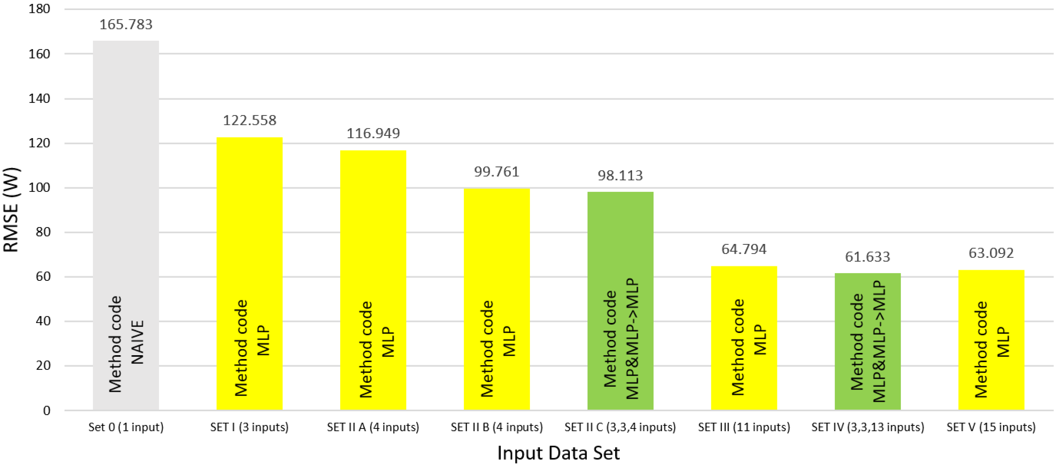
- The smallest RMSE and nMAPE errors were obtained by the MLP method among the seven tested methods (including two group methods), and this method can be considered the preferred one. The RF and IT2FLS methods obtained a slightly higher RMSE error;
- The difference in the quality of forecasts between the best MLP method and the worst NAIVE is quite large;
- The SVR method obtained an RMSE error significantly higher than the best MLP method (according to the RMSE measure), while the nMAPE error was almost identical to the MLP method.
- The use of exogenous variables for forecasts made it possible to reduce the RMSE error of all the methods used;
- The use of smoothed power generation in period t−1 (in SET 2B) as an input variable instead of power generation in period t−1 (in SET 2A) turned out to be beneficial—all tested methods obtained a lower RMSE error;
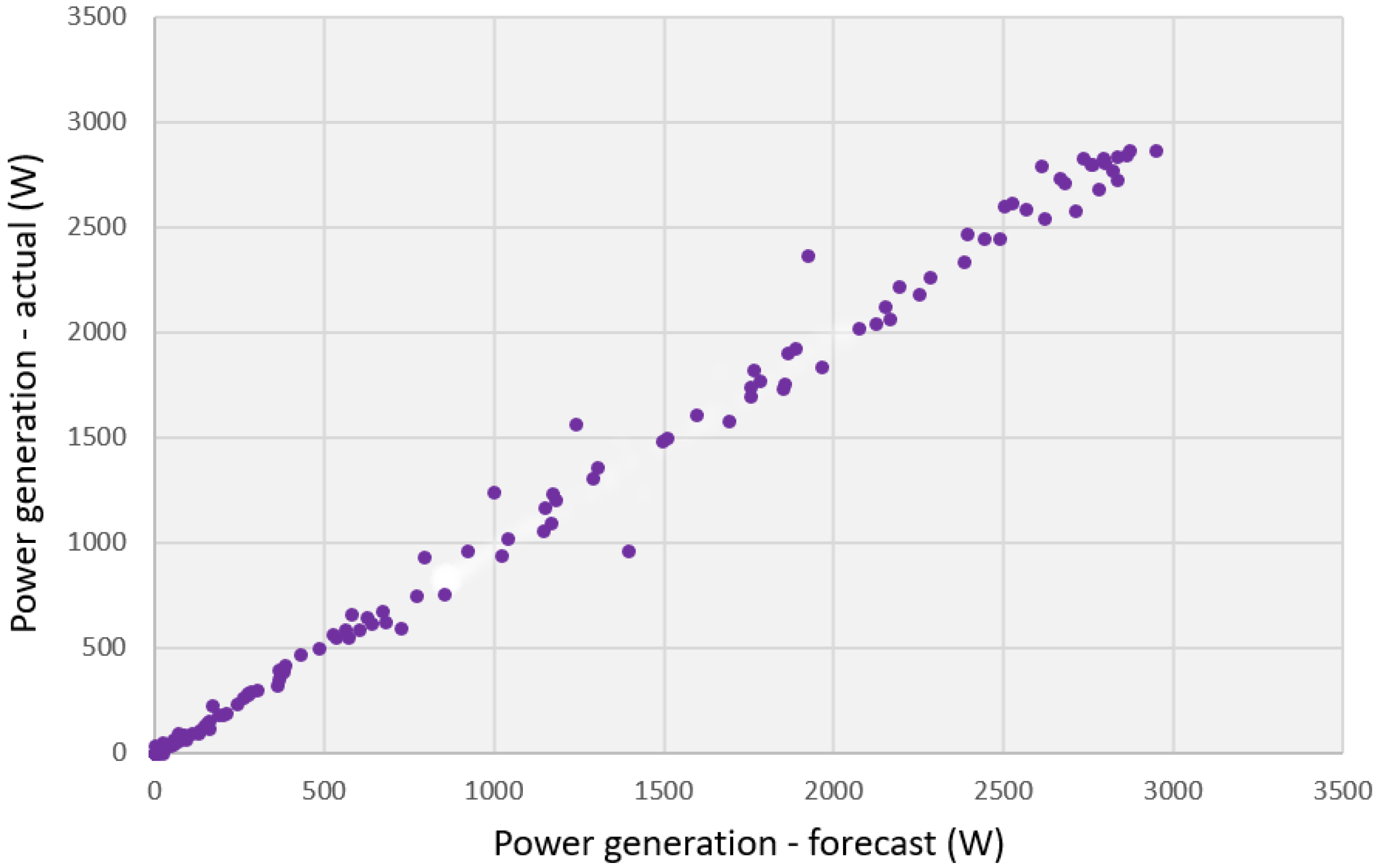
- The smallest RMSE error and nMAPE error were obtained by the original, proprietary hybrid method (MLP&MLP->MLP). On the other hand, the MLP method obtained RMSE and nMAPE errors that were slightly higher;
- The largest RSME error, significantly greater than other methods, was obtained by the reference method—the NAIVE method, while the GBT method was the method with the second-greatest RSME error;
- The SVR method using four sets of input data (including exogenous variables) significantly reduced the RMSE error compared to the forecasts using three sets of input data (only the last two withdrawn values of the forecast process)—see Table 5.
- The use of a larger number of input data, from 11 to 15 for forecasts (including exogenous variables), allowed for a significant reduction in the RMSE error of all methods used compared to the use of only four sets of input data;
- The smallest RMSE error and nMAPE error were obtained by the original, proprietary hybrid method (MLP&MLP->MLP), and it is the recommended method. On the other hand, the MLP method obtained RMSE and nMAPE errors that were slightly higher;
- The largest RSME error, significantly greater than other methods, was obtained by the reference method—the NAIVE method, while the GBT method was the method with the second-greatest RSME error;
- The SVR method using 15 sets of input data (including exogenous variables) was one of the best methods, but the use of 11 sets of input data proved to be less favorable;
- Team methods with different types of predictors in the team (WAE (SVR,MLP) and WAE (LR,MLP)) were also among the best methods—the RMSE error of these methods was slightly greater than the second MLP method in the list;
- For all tested methods, it was more advantageous to use 15 sets of input data than 11 sets of input data.
7. Conclusions
- Increasing the forecast horizon to 1 h (4 forecasts for consecutive 15 min periods);
- Using various techniques for decomposing the prognostic problem and examining their impact on the quality of forecasts (in the case of obtaining data from a period of several years);
- Examining the distribution of forecast errors during the day—verifying whether there is a relationship between the RMSE error rate and the time of day;
- Quality-testing forecasting models using additional solar irradiance, wind speed, and wind direction forecasts (in the case of obtaining such meteorological forecasts).
Author Contributions
Funding
Institutional Review Board Statement
Informed Consent Statement
Data Availability Statement
Acknowledgments
Conflicts of Interest
Abbreviations
| ACF | Autocorrelation Function |
| ANFIS | Adaptive Neuro-Fuzzy Inference System |
| ANN | Artificial Neural Network |
| BFGS | Broyden–Fletcher–Goldfarb–Shanno algorithm |
| C&RT | Classification and Regression Trees algorithm |
| DCs | Decision Trees |
| EIASC | Enhanced iterative algorithm with stop condition |
| GA | Genetic algorithm |
| GBT | Gradient-Boosted Trees |
| GSA | Global sensitivity analysis |
| IASC | Iterative algorithm with stop condition |
| IT2FLS | Interval Type-2 Fuzzy Logic System |
| KM | Karnik–Mendel |
| KNNR | K-Nearest Neighbors Regression |
| LR | Linear Regression |
| MBE | Mean Bias Error |
| MLP | Multi-Layer Perceptron |
| nAPEmax | Normalized Maximum Absolute Percentage Error |
| nMAPE | Normalized Mean Absolute Percentage Error |
| PR | Performance ratio |
| PSO | Particle Swarm Optimization |
| PV | Photovoltaic |
| R | Pearson linear correlation coefficient |
| RES | Renewable Energy Sources |
| R2 | Determination coefficient |
| RF | Random forest |
| RMSE | Root Mean Square Error |
| SVM | Support Vector Machine |
| SVR | Support Vector Regression |
Appendix A

| Method Code | Description of Method, Name, and Range of Values of Hyperparameters’ Tuning and Selected Values |
| SVR | Regression SVM: Type-1, Type 2, selected: Type-1; kernel type: Gaussian (RBF); width parameter σ: 0.333; regularization constant C, range: 1–50 (step 1), selected: 2; tolerance ε, range: 0.01–0.2 (step 0.01), selected: 0.02. |
| KNNR | Number of nearest neighbours k, Distance metrics: Euclidean, Manhattan, Minkowski, selected: Euclidean; range: 1–50, selected: 13. |
| MLP | Learning algorithm: BFGS; the number of neurons in hidden layer: 2–10, selected: 3; activation function in hidden layer: linear, hyperbolic tangent, selected: hyperbolic tangent; activation function in output layer: linear. |
| IT2FLS | Interval Type-2: Sugeno FLS, Mamdani FLS, selected: Sugeno FLS; learning and tuning algorithm: GA, PSO, selected: PSO; initial swarm span: 1500–2500, selected: 2000; minimum neighborhood size: 0.20–0.30, selected: 0.25; inertia range: from [0.10–1.10] to [0.20–2.20], selected: [0.50–0.50]; number of iterations in the learning and tuning process: 5–20, selected: 20; type of the membership functions: triangular, Gauss, selected: Gauss; the number of output membership functions: 3–81, selected: 81; defuzzification method: Centroid, Weighted average of all rule outputs, selected: Weighted average of all rule outputs; AND operator type: min, prod, selected: min; OR operator type: max, probor, selected: probor; implication type: prod, min, selected: min; aggregation type: sum, max, selected: sum; the k-Fold Cross-Validation value: 1–4, selected: 4; window size for computing average validation cost: 5–10, selected: 7; maximum allowable increase in validation cost: 0.0–1.0, selected: 0.1; the type-reduction methods: KM, IASC, EIASC, selected: KM. |
| RF | The number of decision trees: 2–50, selected: 5; the number of predictors chosen at random: 1, 2, selected 2. Stop parameters: maximum number of levels in each decision tree: 5, 10, 20, selected 10; minimum number of data points placed in a node before the node is split: 10, 20, 30, 40, 50, selected 20; minimum number of data points allowed in a leaf node: 10; maximum number of nodes: 100. |
| GBT | Considered max depth: 2/4, selected depth: 2; trees number: 50/100/150/200/250, selected number: 100; learning rate: 0.1/0.01/0.001, selected: 0.1. |
References
- Shamsollahi, P.; Cheung, K.W.; Chen, Q.; Germain, E.H. A neural network based very short term load forecaster for the interim ISO New England electricity market system. In Proceedings of the 2001 Power Industry Computer Applications Conference, Sydney, Australia, 20–24 May 2001; pp. 217–222. [Google Scholar]
- Parol, M.; Piotrowski, P. Very short-term load forecasting for optimum control in microgrids. In Proceedings of the 2nd International Youth Conference on Energetics (IYCE 2009), Budapest, Hungary, 4–6 June 2009; pp. 1–6. [Google Scholar]
- Parol, M.; Piotrowski, P. Electrical energy demand forecasting for 15 minutes forward for needs of control in low voltage electrical networks with installed sources of distributed generation. Przegląd Elektrotechniczny Electr. Rev. 2010, 86, 303–309. (In Polish) [Google Scholar]
- Parol, M.; Piotrowski, P.; Kapler, P.; Piotrowski, M. Forecasting of 10-Second Power Demand of Highly Variable Loads for Microgrid Operation Control. Energies 2021, 14, 1290. [Google Scholar] [CrossRef]
- Hernandez, L.; Baladron, C.; Aguiar, J.M.; Carro, B.; Sanchez-Esguevillas, A.J.; Lloret, J.; Massana, J. A Survey on Electric Power Demand Forecasting: Future Trends in Smart Grids, Microgrids and Smart Buildings. IEEE Commun. Surv. Tutor. 2014, 16, 1460–1495. [Google Scholar] [CrossRef]
- Niu, D.; Pu, D.; Dai, S. Ultra-Short-Term Wind-Power Forecasting Based on the Weighted Random Forest Optimized by the Niche Immune Lion Algorithm. Energies 2018, 11, 1098. [Google Scholar] [CrossRef] [Green Version]
- Bokde, N.; Feijóo, A.; Villanueva, D.; Kulat, K. A Review on Hybrid Empirical Mode Decomposition Models for Wind Speed and Wind Power Prediction. Energies 2019, 12, 254. [Google Scholar] [CrossRef] [Green Version]
- Adnan, R.M.; Liang, Z.; Yuan, X.; Kisi, O.; Akhlaq, M.; Li, B. Comparison of LSSVR, M5RT, NF-GP, and NF-SC Models for Predictions of Hourly Wind Speed and Wind Power Based on Cross-Validation. Energies 2019, 12, 329. [Google Scholar] [CrossRef] [Green Version]
- Würth, I.; Valldecabres, L.; Simon, E.; Möhrlen, C.; Uzunoğlu, B.; Gilbert, C.; Giebel, G.; Schlipf, D.; Kaifel, A. Minute-Scale Forecasting of Wind Power—Results from the Collaborative Workshop of IEA Wind Task 32 and 36. Energies 2019, 12, 712. [Google Scholar] [CrossRef] [Green Version]
- Liu, F.; Li, R.; Dreglea, A. Wind Speed and Power Ultra Short-Term Robust Forecasting Based on Takagi–Sugeno Fuzzy Model. Energies 2019, 12, 3551. [Google Scholar] [CrossRef] [Green Version]
- Carpinone, A.; Giorgio, M.; Langella, R.; Testa, A. Markov chain modeling for very-short-term wind power forecasting. Electr. Power Syst. Res. 2015, 122, 152–158. [Google Scholar] [CrossRef] [Green Version]
- Tato, J.H.; Brito, M.C. Using Smart Persistence and Random Forests to Predict Photovoltaic Energy Production. Energies 2018, 12, 100. [Google Scholar] [CrossRef] [Green Version]
- Zhu, R.; Guo, W.; Gong, X. Short-Term Photovoltaic Power Output Prediction Based on k-Fold Cross-Validation and an Ensemble Model. Energies 2019, 12, 1220. [Google Scholar] [CrossRef] [Green Version]
- Abdullah, N.A.; Rahim, N.A.; Gan, C.K.; Adzman, N.N. Forecasting Solar Power Using Hybrid Firefly and Particle Swarm Optimization (HFPSO) for Optimizing the Parameters in a Wavelet Transform-Adaptive Neuro Fuzzy Inference System (WT-ANFIS). Appl. Sci. 2019, 9, 3214. [Google Scholar] [CrossRef] [Green Version]
- Nespoli, A.; Mussetta, M.; Ogliari, E.; Leva, S.; Fernández-Ramírez, L.; García-Triviño, P. Robust 24 Hours ahead Forecast in a Microgrid: A Real Case Study. Electronics 2019, 8, 1434. [Google Scholar] [CrossRef] [Green Version]
- Ahmed, R.; Sreeram, V.; Mishra, Y.; Arif, M.D. A review and evaluation of the state-of-art in PV solar power forecasting: Techniques and optimization. Renew. Sust. Energ. Rev. 2020, 124, 109792. [Google Scholar] [CrossRef]
- Antonanzas, J.; Osorio, N.; Escobar, R.; Urraca, R.; Martinez-de-Pison, F.J.; Antonanzas-Torres, F. Review of photovoltaic power forecasting. Sol. Energy 2016, 136, 78–111. [Google Scholar] [CrossRef]
- Mayer, M.J.; Gróf, G. Extensive comparison of physical models for photovoltaic power forecasting. Appl. Energy 2021, 283, 116239. [Google Scholar] [CrossRef]
- Mayer, M.J. Influence of design data availability on the accuracy of physical photovoltaic power forecasts. Sol. Energy 2021, 227, 532–540. [Google Scholar] [CrossRef]
- Study Committee: C6; CIGRÉ Working Group C6.22. Microgrids 1: Engineering, Economics, & Experience-Capabilities, Benefits, Business Opportunities, and Examples-Microgrids Evolution Roadmap; Technical Brochure 635; CIGRE: Paris, France, 2015. [Google Scholar]
- Marnay, C.; Chatzivasileiadis, S.; Abbey, C.; Iravani, R.; Joos, G.; Lombardi, P.; Mancarella, P.; von Appen, J. Microgrid evolution roadmap. Engineering, economics, and experience. In Proceedings of the 2015 International Symposium on Smart Electric Distribution Systems and Technologies (EDST15), CIGRE SC C6 Colloquium, Vienna, Austria, 8–11 September 2015. [Google Scholar]
- Microgrids: Architectures and Control; Hatziargyriou, N.D. (Ed.) Wiley-IEEE Press: Hoboken, NJ, USA, 2014. [Google Scholar]
- Baczynski, D.; Ksiezyk, K.; Parol, M.; Piotrowski, P.; Wasilewski, J.; Wojtowicz, T. Low Voltage Microgrids. Joint Publication Edited by Mirosław Parol; Publishing House of the Warsaw University of Technology: Warsaw, Poland, 2013. (In Polish) [Google Scholar]
- Li, Y.; Nejabatkhah, F. Overview of control, integration and energy management of microgrids. J. Mod. Power Syst. Clean Energy 2014, 2, 212–222. [Google Scholar] [CrossRef] [Green Version]
- Olivares, D.E.; Canizares, C.A.; Kazerani, M. A Centralized Energy Management System for Isolated Microgrids. IEEE Trans. Smart Grid 2014, 5, 1864–1875. [Google Scholar] [CrossRef]
- Morstyn, T.; Hredzak, B.; Agelidis, V.G. Control strategies for microgrids with distributed energy storage systems: An overview. IEEE Trans. Smart Grid 2018, 9, 3652–3666. [Google Scholar] [CrossRef] [Green Version]
- Lopes, J.A.P.; Moreira, C.L.; Madureira, A.G. Defining Control Strategies for MicroGrids Islanded Operation. IEEE Trans. Power Syst. 2006, 21, 916–924. [Google Scholar] [CrossRef] [Green Version]
- Parol, M.; Rokicki, Ł.; Parol, R. Towards optimal operation control in rural low voltage microgrids. Bull. Pol. Ac. Tech. 2019, 67, 799–812. [Google Scholar]
- Parol, M.; Kapler, P.; Marzecki, J.; Parol, R.; Połecki, M.; Rokicki, Ł. Effective approach to distributed optimal operation control in rural low voltage microgrids. Bull. Pol. Ac. Tech. 2020, 68, 661–678. [Google Scholar]
- Zakir, M.; Sher, H.A.; Arshad, A.; Lehtonen, M. A fault detection, localization, and categorization method for PV fed DC-microgrid with power-sharing management among the nano-grids. Int. J. Electr. Power Energy Syst. 2022, 137, 107858. [Google Scholar] [CrossRef]
- Sharma, V.; Chandel, S.S. Performance and degradation analysis for long term reliability of solar photovoltaic systems: A review. Renew. Sust. Energ. Rev. 2013, 27, 753–767. [Google Scholar] [CrossRef]
- Makrides, G.; Norton, M.; Georghiou, G.E. Performance of Photovoltaics Under Actual Operating Conditions. Third Gener. Photovolt. 2012, 201–232. [Google Scholar] [CrossRef] [Green Version]
- Dierauf, T.; Growitz, A.; Kurtz, S.; Cruz, J.L.B.; Riley, E.; Hansen, C. Weather-Corrected Performance Ratio; Technical Report; NREL/TP-5200-57991; National Renewable Energy Lab.(NREL): Golden, CO, USA, April 2013. [Google Scholar]
- Nordmann, T.; Clavadetscher, L. Understanding temperature effects on PV system performance. In Proceedings of the 3rd IEEE World Conference on Photovoltaic Energy Conversion, Osaka, Japan, 11–18 May 2003; pp. 2243–2246. [Google Scholar]
- Virtuani, A.; Pavanello, D.; Friesen, G. Overview of Temperature Coefficients of Different Thin Film Photovoltaic Technologies. In Proceedings of the 25th EUPVSEC Conference, Valencia, Spain, 6–10 September 2010. [Google Scholar] [CrossRef]
- Skoplaki, E.; Palyvos, J.A. On the temperature dependence of photovoltaic module electrical performance: A review of efficiency/power correlations. Sol. Energy 2009, 83, 614–624. [Google Scholar] [CrossRef]
- Makrides, G.; Theristis, M.; Bratcher, J.; Pratt, J.; Georghiou, G.E. Five-year performance and reliability analysis of monocrystalline photovoltaic modules with different backsheet materials. Sol. Energy 2018, 171, 491–499. [Google Scholar] [CrossRef]
- Taylor, N. Traceable Performance Measurements of PV Devices; European Union: Luxembourg, 2010. [CrossRef]
- Polo, J.; Alonso-Abella, M.; Ruiz-Arias, J.A.; Balenzategui, J.L. Worldwide analysis of spectral factors for seven photovoltaic technologies. Sol. Energy 2017, 142, 194–203. [Google Scholar] [CrossRef]
- Rahmann, C.; Vittal, V.; Ascui, J.; Haas, J. Mitigation Control Against Partial Shading Effects in Large-Scale PV Power Plants. IEEE Trans. Sustain. Energy 2016, 7, 173–180. [Google Scholar] [CrossRef]
- Géron, A. Hands-on Machine Learning with Scikit-Learn, Keras, and TensorFlow, 2nd ed.; O’Reilly Media, Inc.: Sevastopol, CA, USA, 2019. [Google Scholar]
- Piotrowski, P.; Baczyński, D.; Kopyt, M.; Gulczyński, T. Advanced Ensemble Methods Using Machine Learning and Deep Learning for One-Day-Ahead Forecasts of Electric Energy Production in Wind Farms. Energies 2022, 15, 1252. [Google Scholar] [CrossRef]
- Dudek, G.; Pełka, P. Forecasting monthly electricity demand using k nearest neighbor method. Przegląd Elektrotechniczny Electr. Rev. 2017, 93, 62–65. [Google Scholar]
- Piotrowski, P.; Baczyński, D.; Kopyt, M.; Szafranek, K.; Helt, P.; Gulczyński, T. Analysis of forecasted meteorological data (NWP) for efficient spatial forecasting of wind power generation. Electr. Power Syst. Res. 2019, 175, 105891. [Google Scholar] [CrossRef]
- Dudek, G. Multilayer perceptron for short-term load forecasting: From global to local approach. Neural Comput. Appl. 2019, 32, 3695–3707. [Google Scholar] [CrossRef] [Green Version]
- Osowski, S.; Siwek, K. Local dynamic integration of ensemble in prediction of time series. Bull. Pol. Ac. Tech 2019, 67, 517–525. [Google Scholar]
- Karnik, N.; Mendel, J.; Liang, Q. Type-2 fuzzy logic systems. IEEE Trans. Fuzzy Syst. 1999, 7, 643–658. [Google Scholar] [CrossRef] [Green Version]
- Karnik, N.N.; Mendel, J.M. Centroid of a type-2 fuzzy set. Inf. Sci. 2001, 132, 195–220. [Google Scholar] [CrossRef]
- Mendel, J.; John, R. Type-2 fuzzy sets made simple. IEEE Trans. Fuzzy Syst. 2002, 10, 117–127. [Google Scholar] [CrossRef]
- Khosravi, A.; Nahavandi, S.; Creighton, D.; Srinivasan, D. Interval Type-2 Fuzzy Logic Systems for Load Forecasting: A Comparative Study. IEEE Trans. Power Syst. 2012, 27, 1274–1282. [Google Scholar] [CrossRef]
- Liang, Q.; Mendel, J.M. Interval type-2 fuzzy logic systems: Theory and design. IEEE Trans. Fuzzy Syst. 2000, 8, 535–550. [Google Scholar] [CrossRef] [Green Version]
- Hastie, T.; Tibshirani, R.; Friedman, J.H. The elements of Statistical Learning. Data Mining, Inference, and Prediction, 2nd ed.; Springer: Berlin/Heidelberg, Germany, 2009. [Google Scholar]


| Statistical Measures | PV System Data |
|---|---|
| Mean | 635.61 (W) |
| Percentage ratio of mean power to installed power | 19.86% |
| Standard deviation | 930.63 (W) |
| Minimum | 0.00 (W) |
| Maximum | 3114.81 (W) |
| Range | 3114.81 (W) |
| Coefficient of variation | 146.41% |
| The 10th percentile | 0.00 (W) |
| The 25th percentile (lower quartile) | 0.00 (W) |
| The 50th percentile (median) | 46.91 (W) |
| The 75th (upper quartile) | 1127.19 (W) |
| The 90th percentile | 2368.10 (W) |
| Variance | 866,074.80 (-) |
| Skewness | 1.23 (-) |
| Kurtosis | −0.04 (-) |
| Code of Variable | Potential Explanatory Variables Considered | R |
|---|---|---|
| SPG(T-1) | Smoothed power generation in period t−1 | 0.9756 |
| PG(T-1) | Power generation in period t−1 | 0.9744 |
| PG(T-2) | Power generation in period t−2 | 0.9601 |
| PG(T-3) | Power generation in period t−3 | 0.9536 |
| SI(T-1) | Solar irradiance in period t−1 | 0.9661 |
| SI(T-2) | Solar irradiance in period t−2 | 0.9587 |
| SI(T-3) | Solar irradiance in period t−3 | 0.9385 |
| AT(T-1) | Air temperature in period t−1 | 0.4261 |
| PV_MT(T-1) | PV module temperature in period t−1 | 0.7134 |
| WD(T-1) | Wind direction in period t−1 | −0.2475 |
| WS(T-1) | Wind speed in period t−1 | 0.1825 |
| Name of Set | Codes of Input Data and Additional Comments |
|---|---|
| Set 0 (1 input) | PG(T-1) |
| SET I (3 inputs) | PG(T-1), PG(T-2), PG(T-3) |
| SET II A (4 inputs) | PG(T-1), SI(T-1), PV_MT(T-1), AT(T-1) |
| SET II B (4 inputs) | SPG(T-1), SI(T-1), PV_MT(T-1), AT(T-1) |
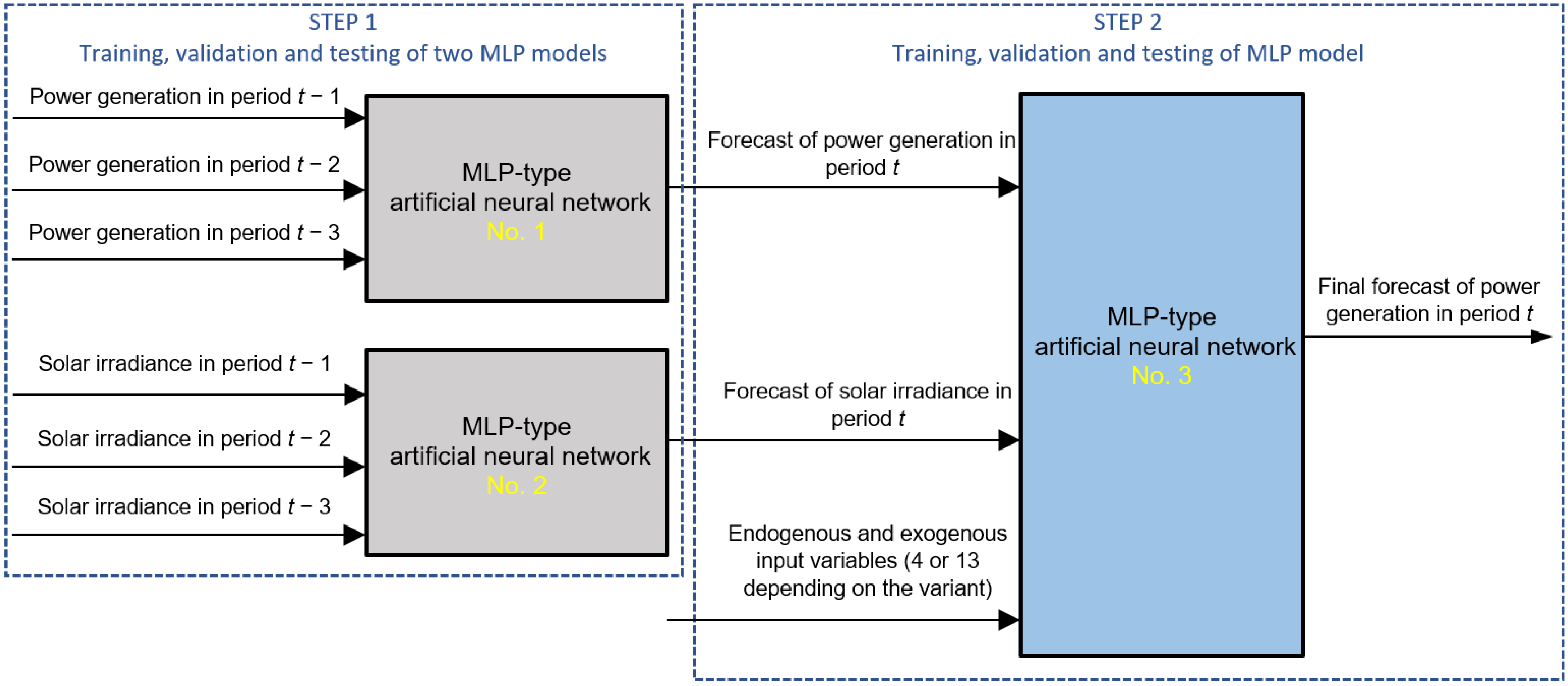
| SET II C (3, 3, 4 inputs) | PG(T-1), PG(T-2), PG(T-3)—inputs for predicting PG forecast(T) SI(T-1), SI(T-2), SI(T-3)—inputs for predicting SI forecast(T) PG forecast(T), SI forecast(T), PV_MT(T-1), AT(T-1)—inputs for predicting PG(T) |
| SET III (11 inputs) | SPG(T-1), PG(T-1), PG(T-2), PG(T-3), SI(T-1), SI(T-2), SI(T-3), AT(T-1), PV_MT(T-1), WD(T-1), WS(T-1) |
| SET IV (3, 3, 13 inputs) | PG(T-1), PG(T-2), PG(T-3)—inputs for predicting PG forecast(T) SI(T-1), SI(T-2), SI(T-3)—inputs for predicting SI forecast(T) SPG(T-1), PG(T-1), PG(T-2), PG(T-3), SI(T-1), SI(T-2), SI(T-3), AT(T-1), PV_MT(T-1), WD(T-1), WS(T-1), PG forecast(T), SI forecast(T)—inputs for predicting PG(T) |
| SET V (15 inputs) | SPG(T-1), PG(T-1), PG(T-2), PG(T-3), SI(T-1), SI(T-2), SI(T-3), AT(T-1), AT(T-2), AT(T-3), PV_MT(T-1), PV_MT(T-2), PV_MT(T-3), WD(T-1), WS(T-1) |
| The Name of Method | The Method Code | Complexity of Method/Type | Tested Sets of Input Data |
|---|---|---|---|
| Persistence model | NAIVE | Single/linear | Set 0 |
| Multiple linear regression model | LR | Single/linear | SET I, SET II A, SET II B, SET III, SET V |
| K-Nearest Neighbors Regression | KNNR | Single/non-linear | SET I, SET II A, SET II B, SET III, SET V |
| MLP-type artificial neural network | MLP | Single/non-linear | SET I, SET II A, SET II B, SET III, SET V |
| Support Vector Regression | SVR | Single/non-linear | SET I, SET II A, SET II B, SET III, SET V |
| Interval Type-2 Fuzzy Logic System | IT2FLS | Single/non-linear | SET I, SET II A, SET II B |
| Random forest regression | RF | Ensemble/non-linear | SET I, SET II A, SET II B, SET III, SET V |
| Gradient-Boosted Trees for regression | GBT | Ensemble/non-linear | SET I, SET II A, SET II B, SET III, SET V |
| Weighted Averaging Ensemble | WAE (p1 *, …, pm) | Ensemble/non-linear | SET I, SET IIB, SET III |
| Hybrid method—connection of three MLP models | MLP&MLP→MLP | Hybrid/non-linear | SET II C, SET IV |
| Method Code | Input Data Set | RMSE (W) | nMAPE (%) | nAPEmax (%) | MBE (W) |
|---|---|---|---|---|---|
| MLP | SET I (3 inputs) | 122.558 | 1.474 | 32.781 | −4.539 |
| WAE [MLP,RF] | SET I (3 inputs) | 129.491 | 1.527 | 30.847 | −2.623 |
| RF | SET I (3 inputs) | 133.931 | 1.674 | 28.439 | −6.832 |
| IT2FLS | SET I (3 inputs) | 135.965 | 1.773 | 29.808 | −6.536 |
| KNNR | SET I (3 inputs) | 137.828 | 1.533 | 33.802 | −5.291 |
| LR | SET I (3 inputs) | 140.989 | 1.617 | 34.214 | 9.711 |
| SVR | SET I (3 inputs) | 142.441 | 1.481 | 34.426 | −3.364 |
| GBT | SET I (3 inputs) | 154.257 | 1.948 | 29.019 | 6.427 |
| NAIVE * | SET 0 (1 input) | 165.783 | 1.975 | 40.199 | −9.030 |
| Method Code | Input Data Set | RMSE (W) | nMAPE (%) | nAPEmax (%) | MBE (W) |
|---|---|---|---|---|---|
| MLP&MLP→MLP | SET II C (3, 3, 4 inputs) | 98.113 | 1.336 | 19.110 | −0.192 |
| MLP | SET 2B (4 inputs) | 99.761 | 1.393 | 18.100 | −6.335 |
| WAE[SVR,MLP] | SET 2B (4 inputs) | 101.825 | 1.423 | 17.743 | −0.098 |
| SVR | SET 2B (4 inputs) | 104.942 | 1.506 | 16.329 | −0.638 |
| WAE[IT2FLS,MLP] | SET 2B (4 inputs) | 105.274 | 1.535 | 18.784 | −0.116 |
| IT2FLS | SET 2B (4 inputs) | 110.461 | 1.540 | 19.223 | 4.956 |
| KNNR | SET 2B (4 inputs) | 116.924 | 1.837 | 19.328 | 6.615 |
| MLP | SET 2A (4 inputs) | 116.949 | 1.715 | 26.040 | −2.637 |
| RF | SET 2B (4 inputs) | 117.383 | 1.632 | 23.882 | −0.142 |
| KNNR | SET 2A (4 inputs) | 118.985 | 1.506 | 27.016 | 4.145 |
| IT2FLS | SET 2A (4 inputs) | 121.590 | 1.661 | 27.173 | 7.511 |
| LR | SET 2B (4 inputs) | 123.803 | 1.961 | 19.513 | −8.993 |
| SVR | SET 2A (4 inputs) | 124.312 | 1.695 | 30.977 | 6.775 |
| GBT | SET 2B (4 inputs) | 124.747 | 1.914 | 17.422 | −9.287 |
| RF | SET 2A (4 inputs) | 129.469 | 1.676 | 28.658 | 11.728 |
| LR | SET 2A (4 inputs) | 132.943 | 2.076 | 27.148 | −2.051 |
| GBT | SET 2A (4 inputs) | 134.457 | 1.914 | 28.318 | −4.637 |
| NAIVE * | SET 0 (1 input) | 165.783 | 1.975 | 40.199 | −9.030 |
| Method Code | Input Data Set | RMSE (W) | nMAPE (%) | nAPEmax (%) | MBE (W) |
|---|---|---|---|---|---|
| MLP&MLP→MLP | SET IV (3,3,13 inputs) | 61.633 | 0.805 | 13.918 | 1.196 |
| MLP | SET V (15 inputs) | 63.092 | 0.848 | 12.375 | −3.498 |
| MLP | SET III (11 inputs) | 64.794 | 0.809 | 16.173 | 3.664 |
| WAE (SVR,MLP) | SET V (15 inputs) | 65.391 | 0.832 | 12.397 | −0.053 |
| SVR | SET V (15 inputs) | 71.618 | 0.824 | 12.629 | −6.088 |
| WAE (LR,MLP) | SET III (11 inputs) | 71.884 | 0.826 | 15.038 | −0.048 |
| SVR | SET III (11 inputs) | 90.379 | 1.416 | 16.065 | 3.570 |
| LR | SET V (15 inputs) | 90.491 | 1.015 | 14.982 | −0.049 |
| LR | SET III (11 inputs) | 91.674 | 1.030 | 21.215 | −3.760 |
| KNNR | SET V (15 inputs) | 104.505 | 1.360 | 18.228 | −4.819 |
| RF | SET V (15 inputs) | 111.269 | 1.577 | 22.362 | −2.483 |
| RF | SET III (11 inputs) | 116.497 | 1.619 | 23.848 | 3.406 |
| KNNR | SET III (11 inputs) | 118.490 | 1.565 | 23.348 | 7.507 |
| GBT | SET V (15 inputs) | 118.547 | 1.523 | 20.386 | −0.179 |
| GBT | SET III (11 inputs) | 122.569 | 1.587 | 25.624 | −2.750 |
| NAIVE * | SET 0 (1 input) | 165.783 | 1.975 | 40.199 | −9.030 |
Publisher’s Note: MDPI stays neutral with regard to jurisdictional claims in published maps and institutional affiliations. |
© 2022 by the authors. Licensee MDPI, Basel, Switzerland. This article is an open access article distributed under the terms and conditions of the Creative Commons Attribution (CC BY) license (https://creativecommons.org/licenses/by/4.0/).
Share and Cite
Piotrowski, P.; Parol, M.; Kapler, P.; Fetliński, B. Advanced Forecasting Methods of 5-Minute Power Generation in a PV System for Microgrid Operation Control. Energies 2022, 15, 2645. https://doi.org/10.3390/en15072645
Piotrowski P, Parol M, Kapler P, Fetliński B. Advanced Forecasting Methods of 5-Minute Power Generation in a PV System for Microgrid Operation Control. Energies. 2022; 15(7):2645. https://doi.org/10.3390/en15072645
Chicago/Turabian StylePiotrowski, Paweł, Mirosław Parol, Piotr Kapler, and Bartosz Fetliński. 2022. "Advanced Forecasting Methods of 5-Minute Power Generation in a PV System for Microgrid Operation Control" Energies 15, no. 7: 2645. https://doi.org/10.3390/en15072645
APA StylePiotrowski, P., Parol, M., Kapler, P., & Fetliński, B. (2022). Advanced Forecasting Methods of 5-Minute Power Generation in a PV System for Microgrid Operation Control. Energies, 15(7), 2645. https://doi.org/10.3390/en15072645