A Multi-Variable DTR Algorithm for the Estimation of Conductor Temperature and Ampacity on HV Overhead Lines by IoT Data Sensors

Abstract

The transfer capabilities of High-Voltage Overhead Lines (HV OHLs) are often limited by the critical power line temperature that depends on the magnitude of the transferred current and the ambient conditions, i.e., ambient temperature, wind, etc. To utilize existing power lines more effectively (with a view to progressive decarbonization) and more safely with respect to the critical power line temperatures, this paper proposes a Dynamic Thermal Rating (DTR) approach using IoT sensors installed on some HV OHLs located in different Italian geographical locations. The goal is to estimate the OHL conductor temperature and ampacity, using a data-driven thermo-mechanical model with the Bayesian probability approach, in order to improve the confidence interval of the results. This work highlights that it could be possible to estimate a space-time distribution of temperature for each OHL and an increase in the actual current threshold values for optimizing OHL ampacity. The proposed model is validated using the Monte Carlo method.

1. Introduction

Over the last few years, several companies operating in the manufacturing and energy management domains have expressed relevant business needs that can be successfully addressed by using Industrial Internet of Things (IIoT) technology. There has been a dramatic increase in the attention paid by the international scientific community to the research topic of the emerging applications of IIoT, especially those aimed at fostering the adoption of cloud- and edge-computing resources [1] as well as of 5G/6G mobile networks. Ranging from data collection to data preparation and analytics to distributed control systems relying on smart sensors, IIoT is indeed expected to provide increased connectivity and a significantly higher degree of automation.

For instance, IIoT has offered the opportunity of setting the stage for the solution of sampled-data nonlinear control problems in the presence of transmission delays [2], of performing effective anomaly detection in production factories [3], of adopting control actions for the protection of power transmission grids from cyber-physical attacks [4], and of performing efficient load balancing in smart grids in a game-theoretic fashion [5].

In this work, we focus on exploiting the potential of IIoT in terms of using existing power lines more effectively (with a view to progressive decarbonization) and more safely with respect to critical power line temperatures.

One of the main causes of the transformation of the Italian electricity grid is certainly the rapid and widespread expansion of renewable source plants, with particular attention to generation from wind, photovoltaic, and hydroelectric sources. This characterizes the evolution of the electricity production park in the last decade, both in Italy and in Europe. The highly distributed nature of these energy sources means that the user, in exchanging energy flows, is not only a consumer but also a producer, thus becoming an active node in the network. The injection into the power grid occurs most of the time in areas of the grid with an unknown magnitude of power, due to the non-programmability of renewable sources. To achieve the national decarbonization purpose, digitalization and innovation of the network are needed. The keys are electrical infrastructures as an integrated system for monitoring the environment with innovative digital tools placed on the pylons and the support of IIoT technologies.

DTLR (Dynamic Thermal Line Rating) systems are classified as indirect and direct methods. Indirect methods measure data related to the weather [6,7], whereas direct methods measure data such as conductor sag [8], conductor ground clearance [9,10,11], line tension [12,13], or even conductor temperature [14,15].

In ref. [16], considering the emerging scenarios of RES (Renewable Energy Source) installation, DTR is taken into account as a method for connecting the new intermittent generation, thus allowing to increase the rating of non-thermally limited lines (long lines). In ref. [17], the paper discusses the wide range of real-time line monitoring devices, which can be used to determine the DTR of an overhead transmission line in normal or contingency operation. In ref. [18], the dynamic values of the line current are assessed as a function of any variations due to the high penetration of intermittent RES in those cases when significant forecasting errors happen. In ref. [19], an optimal algorithm is proposed for the management of congestion on the electric transmission system in real time, considering the quasi-dynamic thermal rates of transmission lines. In refs. [20,21], several types of commercially available DTR systems are taken into account, and the results from the use of DTR systems with respect to a real-world 220 kV connection are shown.

This work proposes a dynamic thermo-mechanical model approach that utilizes weather data measured by IoT sensors, through which the conductor’s temperature and ampacities of power grids can be properly estimated. A significant enhancement in the transmission ampacity of power grids was observed when the thermo-mechanical approach was used. Moreover, for the validation of this dynamic model, the Monte Carlo simulation of weather input data is used.

The paper consists of four sections. Section 2 describes source data, the thermal and mechanical methodology, the Bayes approach, and the Monte-Carlo validation. In Section 3, the results of a case study are presented and analyzed. The last section provides the major conclusions and indicates the directions for our future studies.

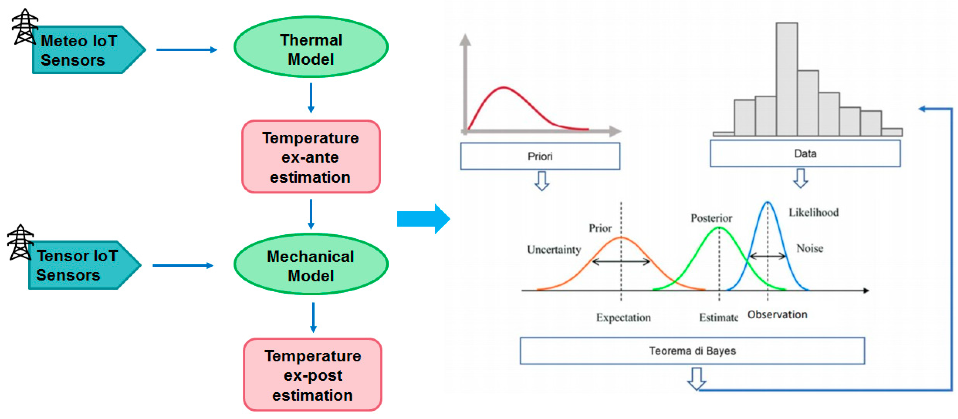
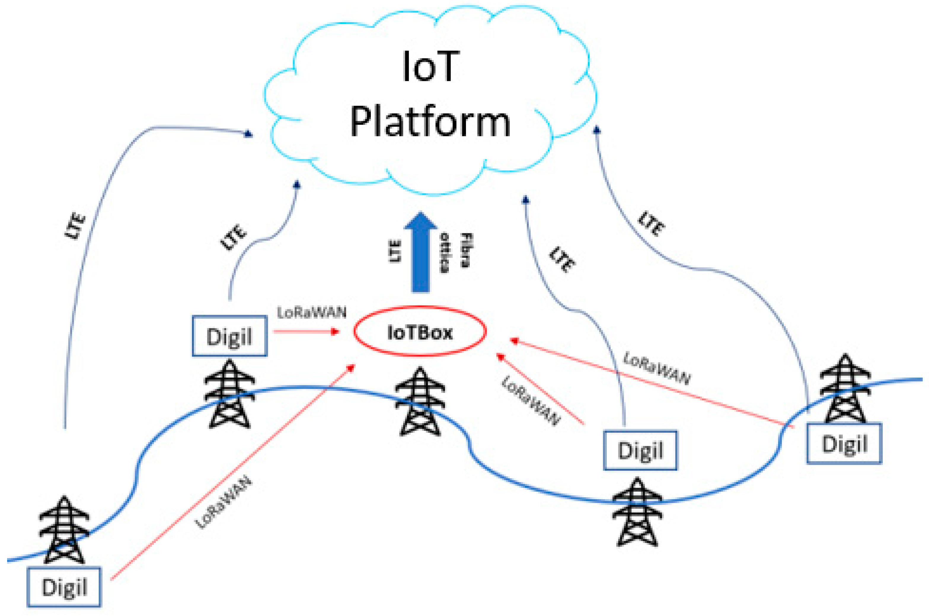
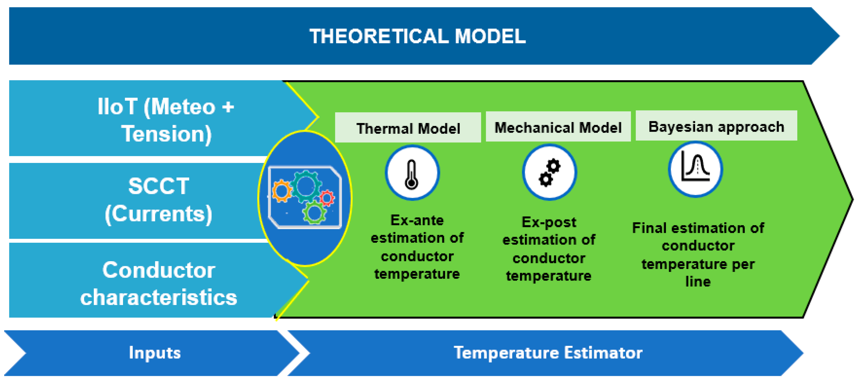
2. Materials and Methods

Data collection is made by an infrastructure, which is based on a wireless sensor network. These sensors (Digil) are installed directly on the pylons of the lines and send the collected data to a concentrator (IoTBox) with a star topology network. IoTBoxes send the recorded measurements with an aggregation time of 15 min. The data are sent finally from the IoTBox to the central processing platform, as shown in Figure 1:

• Weather unit: measurements of wind speed and direction, irradiation, ambient temperature, and relative humidity of the air;
• Mechanical sensors: tension monitoring on the 3 phases, measurement of acceleration/vibration, and inclination of the trellis.

Atmospheric agents represent a considerable problem for overhead lines; therefore, the use of IoT sensor system allows monitoring assets and manages events more effectively. Furthermore, the data provided by the sensors can be used to analyze and estimate the quantities of primary importance for OHL from the point of view of transits and safety parameters. The ampacity of OHL is closely related to conductor temperature, in a view of increasing the capacity of the lines and is defined as the maximum electric current that a conductor can carry continuously before deterioration. The current range is limited by several factors: the structure and the geometry of conductors, the surrounding environmental conditions, and the operating conditions of the line.

The temperature of the conductors depends on the current and local meteorological conditions; therefore, the dynamic evaluation of the range of an overhead line requires the estimation of the maximum time interval in which the line can withstand a given load current.

The most substantial restriction on power delivery via an Extra-High Voltage (EHV) grid is the thermal limit of the line conductor. The indirect measurement of the conductor temperature can be performed by using two analytical models:

• A thermal model, from which we derive an ex ante estimate;
• A mechanical model, from which we derive an ex post estimate.

Thanks to the combination of these two estimations, it is possible to create a temperature probability distribution (Bayesian approach), characterized by a certain degree of confidence.

2.1. Thermal Balance Equation

The thermal balance equation is used to shed light on the relation among the ampacity of a line conductor, conductor temperature, and weather conditions [22,23]. According to the IEEE Std. 738-2006 [22], the relation between the conductor current and the temperature can be expressed by means of a thermal balance equation of gains and losses in terms of heat in the conductor (per unit length):

$$P_j+P_S=P_c+P_r$$

(1)

• P_j = heat generated inside the conductor due to the Joule effect (W/m);
• P_s = density of heat transmitted to the conductor by solar radiation (W/m);
• P_c = density of heat dissipated by convection (W/m);
• P_r = density of heat dissipated by radiation (W/m);

where all the physical quantities and their units in (1) are defined in [22].

2.2. Mechanical Model

Most of the conductors used on overhead lines are made of a core and a mantle of different metal materials. By exposing the conductor to a heat source or applying a tension force, it tends to stretch proportionally to the elastic modulus (E) or to the thermal expansion coefficient (α) of the material it is made of. To maintain the integrity of the conductor, the stretch of the two components must be the same, but the thermal expansion coefficients α of the two materials are different; therefore, the tension stress is distributed differently on both the internal and external parts of the conductor.

The stretching of the conductor leads to a condition where the thermal expansion of the mantle is compensates elastic deformation due to the mechanical state; therefore, the tensile stress is completely transferred on the core and the mantle and is mechanically unloaded.

The temperature at which this passage takes place is defined as the transition temperature; for temperatures higher than the transition one, in fact, all loads are supported by the core of the conductor, which is mechanically deformed and possesses a mass equal to that of the entire conductor and coefficients E and α equal to those of the core one.

For the lines examined, the operating temperature of conductors θ is always lower than the transition temperature; therefore, it is possible to define the equation of the changing steady state of the conductors at high temperatures. The equation describes the mechanical stress variation of spans a, using the measure of the tension force T, coming from the sensors placed on every phase of the conductors.

$$\frac{a^2}{24}\left[{\left(\frac{p}{T_d}\right)}^2-{\left(\frac{p}{T_b}\right)}^2\right]=\frac{T_d-T_b}{E\cdot A}+\alpha \left({\theta }_d-{\theta }_b\right)$$

(2)

• ${\theta }_d:$temperature estimated with the mechanical model (t) (°C)
• ${\theta }_b$: conductor temperature estimated with thermal model (t − 1) (°C)
• E = modulus of elasticity of the conductor (daN/mm²)
• α = thermal expansion coefficient of the conductor (1/°C)
• t: time of variable estimation
• T_d: conductor tension (t) (kN)
• T_b: conductor tension (t − 1) (kN)
• a: span length (m)
• p: unitary transverse actions acting on the conductor (daN/m)

Equation (2) is expressed with temporal references (t); in fact, there are base terms referring to the past temporal (t − 1) step (T_b,θ_b) and derivate terms referring to the actual temporal step (T_d,θ_d).

Using an iterative method, it is possible to calculate the temperature of the conductor ${\theta }_d$ at every time step. For the variation of the mechanical state, it is important to define a starting point from which the state’s change can be evaluated. This point is represented by the ex ante estimate temperature ${\theta }_b$, made by the thermal method, which was inserted as the input of Equation (2) as the best approximation of the conductor’s temperature at the previous time step. The methodological flow used has been represented in Figure 2.

To determine θ_c, it is possible to apply the equation of the change of state (2).

2.3. Bayesian Approach

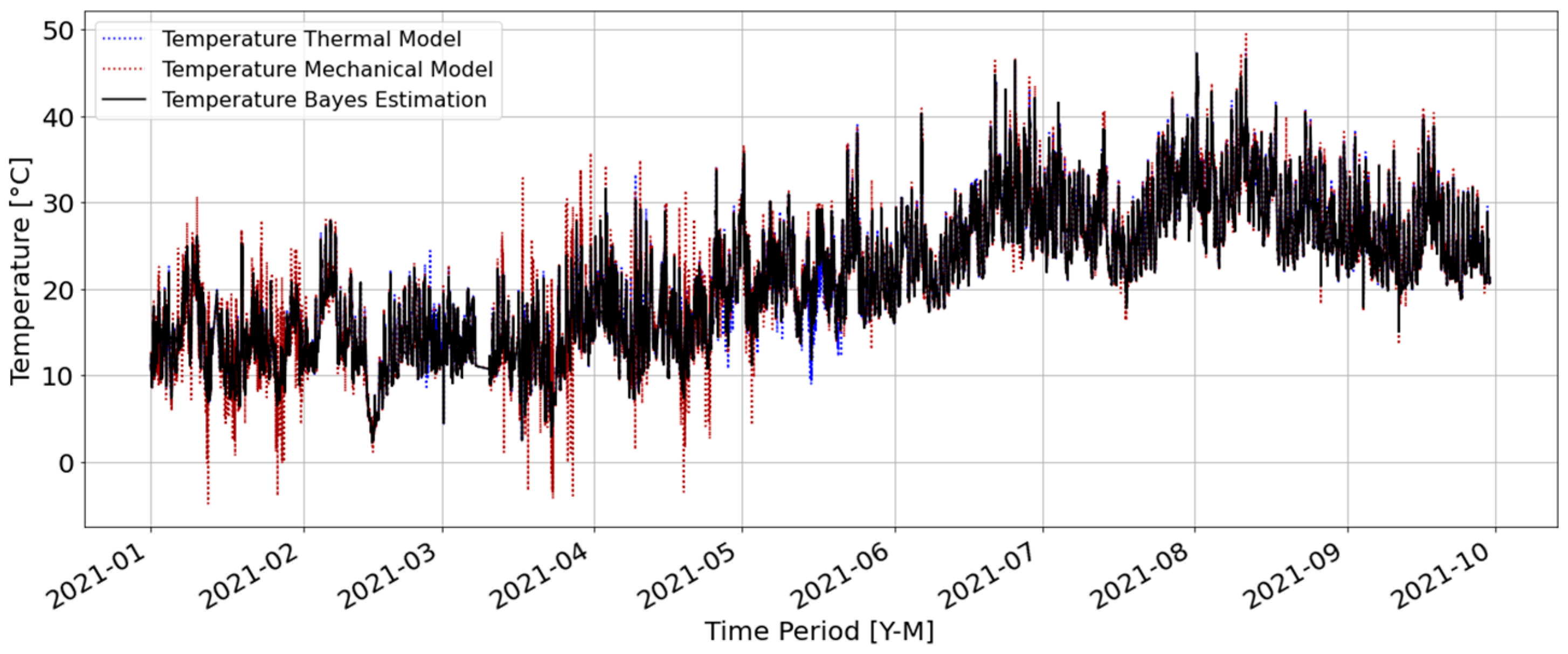
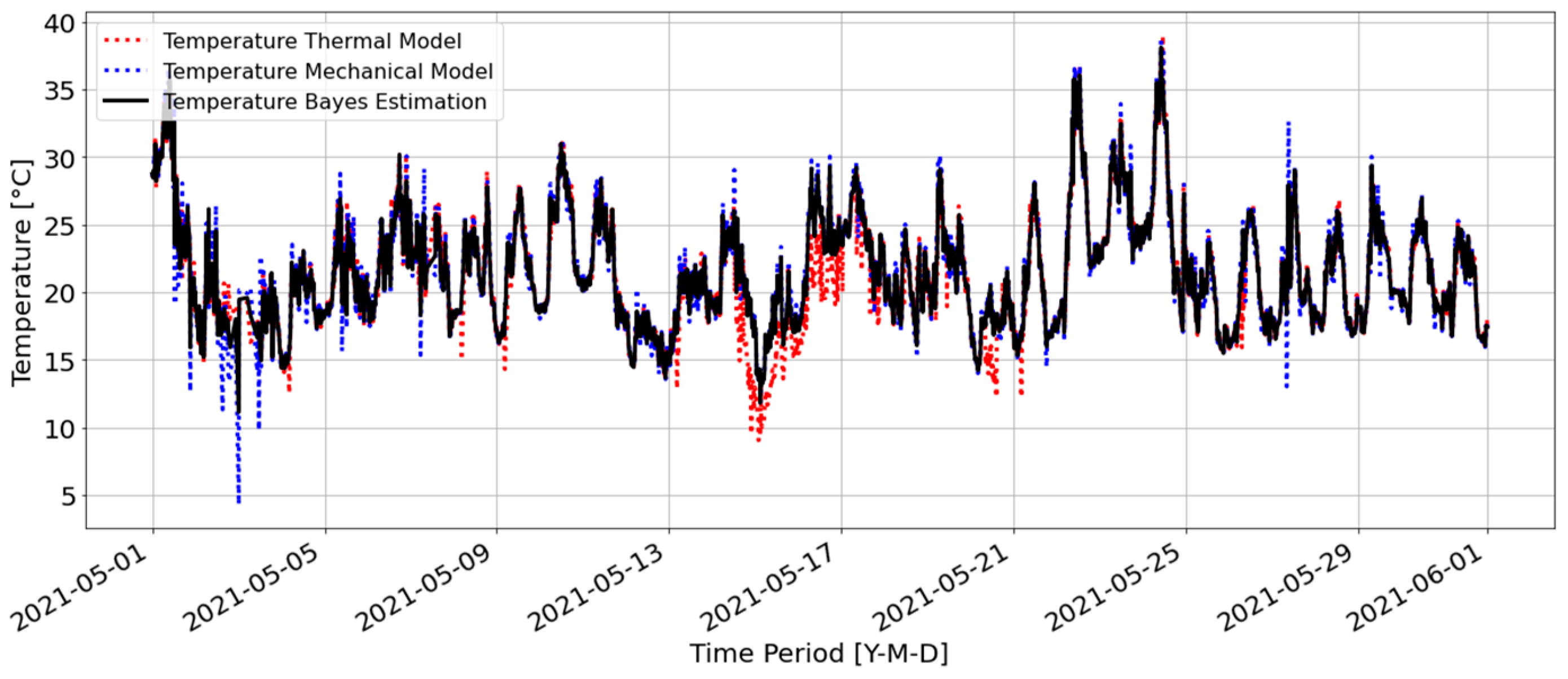
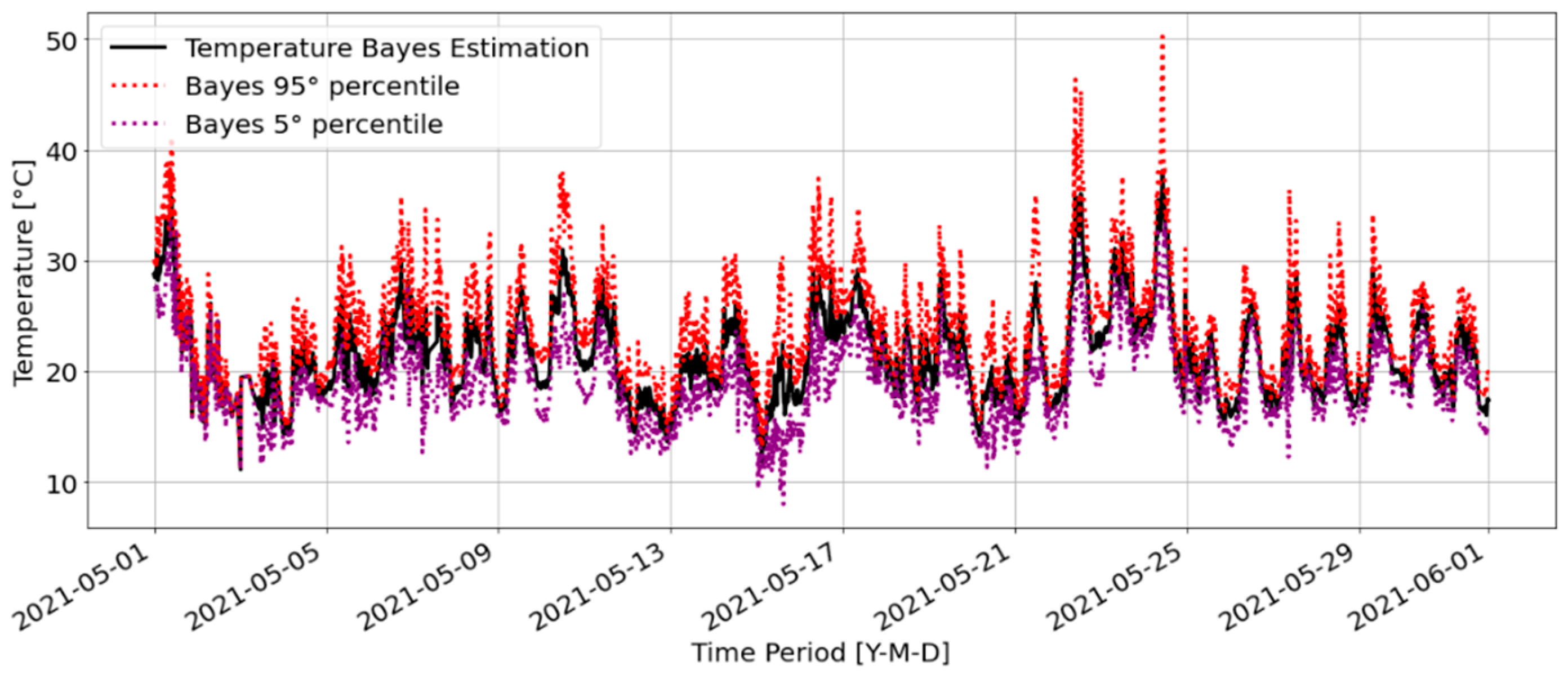
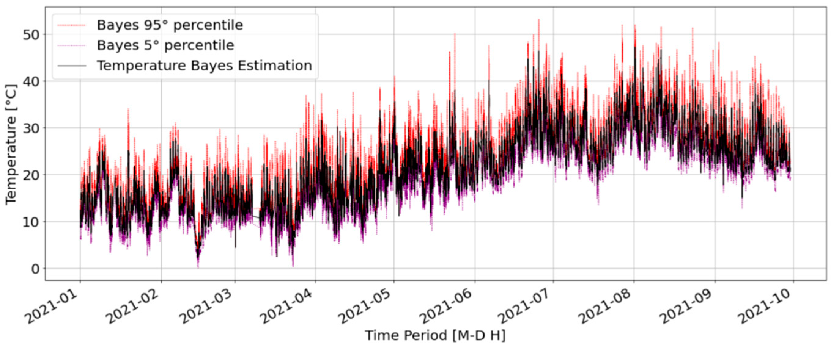
In the Bayesian approach, a certain probability is assigned to a given event before carrying out the experiment (ex ante) established in a subjective way. After observing the experimental frequencies, the a priori probability is modified to arrive at the ex post probability, and it is not an absolute probability but is always conditional.

The Bayesian approach allows the identification of a mean value (3) and standard deviation (4) of the conductor temperature for each line.

The parameters calculated with the generalized Bayes equations describe the Gaussian distribution with which the probability distribution of the conductor temperature is represented for each time interval. The final estimation, therefore, has both a temporal and spatial distribution, to which a certain degree of confidence is attributed.

$${\mu }_{\mathrm{estimated}}=\frac{\left({\mu }_{ante} {\sigma }_{post}^2+{\mu }_{post} {\sigma }_{ante}^2\right)}{{\sigma }_{ante}^2+{\sigma }_{post}^2 }$$

(3)

$${\mathsf{\Sigma }}_{\mathrm{estimated}}=\sqrt{\frac{{\sigma }_{ante}^2{\sigma }_{\mathrm{post}}^2}{{\sigma }_{ante}^2+{\sigma }_{\mathrm{post}}^2}}$$

(4)

In Figure 3, the complete methodology applied for the derivation of the conductor temperature is reported.

3. Results

3.1. Evaluation of Conductor Temperature

According to IEEE Std 738 [22], the conductor temperature is an important parameter, which will directly influence the limit of the current that flows through the line.

At the theoretical level, data from IoT sensors were used as input data for the realization of the model (Figure 4). These include Meteo and Tension data, SCCT Current data, and geometric-physical characteristics of conductors. All these data were used for the implementation of the thermal model (Section 2.1) and also in the mechanical model (Section 2.2). The output temperature of the thermal model (ex ante) was used as the input of the mechanical model that return ex post temperatures. Once the two temperatures were estimated, they were combined with the Bayesian approach with the aim of obtaining the final estimate of the conductor temperature for the entire line (spatial distribution).

Once the model in Error! Reference source not found. has been applied, we obtained the following results.

In Figure 5 and Figure 6, the mean value of the temperature of the considered HV Italian line coming from the thermal model (dashed blue line) is represented, together with the mean value of temperature coming from the mechanical model (dashed red line), as well as the mean value of Bayesian temperature (black line).

The temperature value deriving from the thermal model differs from the temperature value obtained from the mechanical model by an average value (in absolute value) of about 2 degrees.

In Figure 7 and Figure 8, it is possible to observe the estimation of the temperature for an HV Italian line derived from the generalized Bayes equation (black line), for which a 95% confidence range has been attributed.

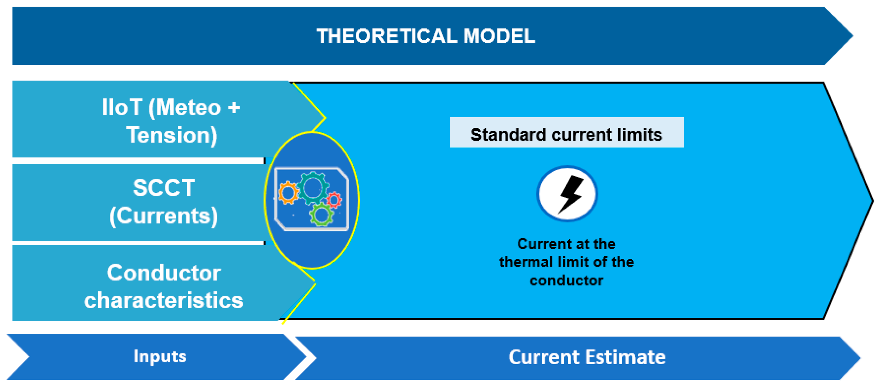
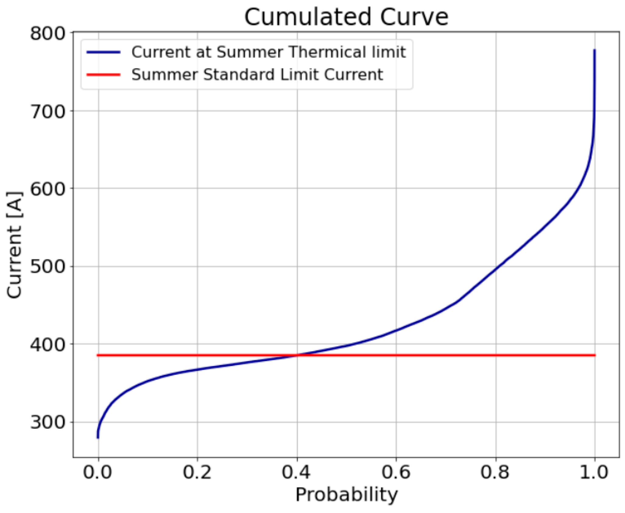
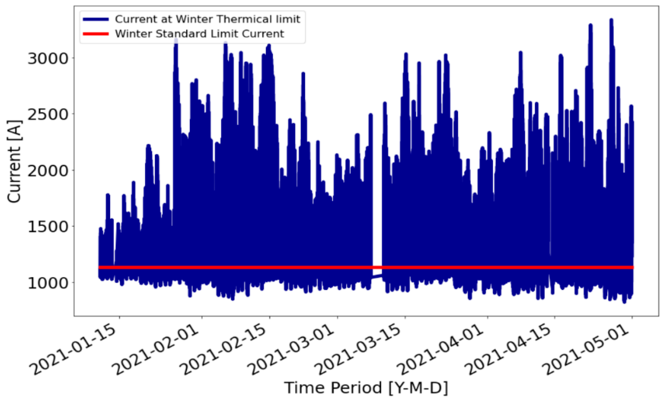
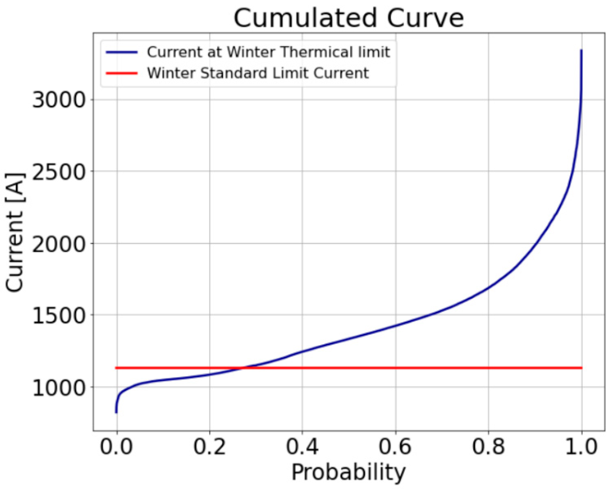
3.2. Evaluation of Ampacity

The use of the theoretical model for the evaluation of ampacity is the same of the temperature estimation model described before. In Figure 9, the input data being used are shown: IoT sensors, Meteo and Tension data, SCCT Current data, and geometric-physical characteristics of conductors. In this work, the authors did not add, as input data, the conductor distance from the ground (mechanical constraint).

Usually, ampacity is used similarly to threshold values derived from a technical catalog: It is calculated without considering the weather conditions associated with the different localization of the lines; the only characterization is the generic division into summer and winter period.

For the determination of optimized ampacity, an ampacity value for each line must be identified, because the limit current value depends on the weather parameters around the pylons.

To overcome this problem and obtain ad hoc limit current values for each line, the DTR model was exploited by setting the temperature of the limit conductor to T_cl = 75 °C. This value represents the limit temperature tolerable by the conductor’s material. The limit current associated with each line will be selected as the minimum current value between the three conductors of the HV Line for each side of the pylon, calculated for every point of measure on the line. This value is evaluated for each timestamp and for each line.

Figure 10 shows the current trend for the summer period of a generic HV Line; Figure 11 shows the cumulate current value for summer period of a generic HV Line; Figure 12 shows the current trend for winter period of a generic HV Line; and at last, Figure 13 presents the cumulate current value for winter period of a generic HV Line.

In Figure 10 and Figure 12, the first evidence of the results is the conductor current range reached at the imposed thermal limit, which is much higher than the current values required by the standard.

In Figure 11 and Figure 13, it is worth noting that, in a significant period of time, it could be possible to increase the actual current threshold values to optimize OHL ampacity. Considering all the lines analyzed, on average, it is optimizable for 17% on summer periods and 44% on winter periods (

Table 1. Outputs obtained for each line analyzed and the average values obtained.

Lines	Standard Value Thermal Model	Standard Value Mechanical Model	Mean Standard Deviation Bayes	Mean Diff Bayes 95	Std Diff Bayes 95	Cumulated Winter	Cumulated Summer	Mean Summer Limit	Mean Winter Limit
1	1.980	2.527	1.342	4.911	2.783	28.429	8.266	369.274	463.147
2	1.010	1.137	0.615	2.250	2.504	40.205	3.694	172.560	103.157
3	1.230	2.827	0.921	3.370	2.462	34.174	6.993	288.907	398.028
4	1.298	1.445	0.872	3.191	2.660	50.753	20.459	71.782	79.996
5	0.795	0.870	0.516	1.887	2.318	47.527	24.429	54.273	88.309
6	1.463	1.736	1.015	3.717	3.042	64.274	40.096	83.131	89.161
mean	1.296	1.757	0.880	3.221	2.628	44.227	17.323	173.321	203.633

).

Table 1 shows the outputs obtained from analyses carried out on each line. Variables ‘mean_diff_bayes_95’ and ‘std_diff_bayes_95’, respectively, represent the mean and standard deviation of the difference between the value of bayes temperature (°C) and the value of 95° percentile. Variables ‘cumulated_summer’ and ‘cumulated_winter’ represent the intersection (evaluated as a percentage of the total time) between the cumulative curve of the calculated ampacities and the standard current limit for the summer and winter periods, respectively. Instead, variables ‘mean_summer_limit’ and ‘mean_winter_limit’ represent the average of the differences between the calculated current (A) and the thermal limit’s current (A) for the summer and winter periods, respectively.

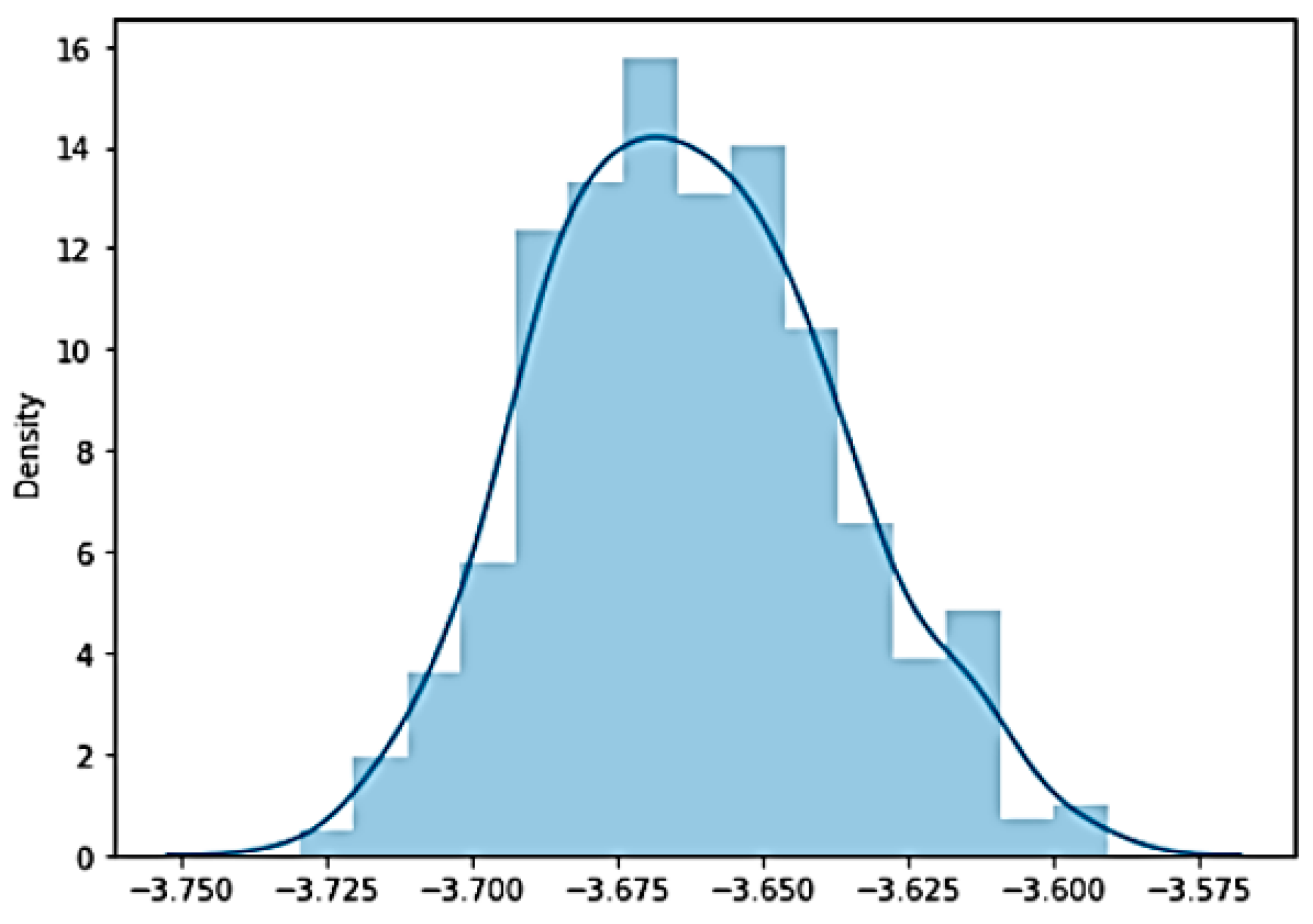
3.3. Monte Carlo Validation

The validation of the model is based on the Monte Carlo method (a computational method based on random sampling to obtain numerical results). For each value measured by the sensors, the average value ($\overline{x}$) and its standard deviation (σ) were computed. With these parameters, the normal distribution associated with each sensor was obtained (refer to

Table 2. Sensors’ accuracy.

Sensor	Accuracy
wind speed (km/h)	if <35: 0.02 * wind_speed, else: 0.03 * wind_speed
wind direction (°)	±2 + wind_direction
air temperature (°C)	±0.15 ± 0.1 * air_temperature
relative humidity (%)	±(1.5 + 1.5 * humidity)
solar radiation (W/m2)	10 ± 1 * solar_heating
ST401Sy datasheet160221 (kN)	±1 * sensor_pull
ST413 datasheet160221 (kN)	±1 * sensor_pull
ST461.1 datasheet160221 (kN)	±1 * sensor_pull
ST461.2 datasheet160221 (kN)	±1 * sensor_pull

and Figure 14 for further detail). Randomly, a large number of values (about 500) were extracted from the normal distributions obtained every 15 min. These extractions represent the input data that allow calculations for a high number of times (namely, equal to the number of values taken from the normal distributions) and for the temperatures of the conductor for every single quarter of an hour. The values found were then averaged, obtaining the mean temperature (T_m) and the mean standard deviation (σ_m).

For the values of the absorption (ε) and emission (α) coefficients, the Monte Carlo method was applied, as previously discussed, obtaining normal distributions starting from an average value of $\overline{x}$ = 0.5 and standard deviation of σ = 0.01.

Table 3. Results of temperature (°C) value obtained before and after the application of Monte Carlo methods.

Timestamp	Montecarlo	Model	Difference
0	−3.168	−3.200	0.032
1	−2.874	−2.900	0.026
2	−1.170	−1.200	0.030
3	−0.565	−0.600	0.035
4	−3.701	−3.700	0.001
5	−3.173	−3.200	0.027
6	−1.071	−1.100	0.029
7	−0.681	−0.700	0.019
8	−3.530	−3.600	0.070
9	−3.600	−3.600	0.000
10	−1.667	−1.700	0.033
11	−0.677	−0.700	0.023
12	−2.900	−2.900	0.000
13	−3.374	−3.400	0.026
14	−2.135	−2.200	0.065

shows the results obtained with the application of the Monte Carlo method (‘montecarlo’ column), and the results from the model without having applied the Monte Carlo Method (‘model’ column). The average of the differences (‘difference’ column) between the values obtained is around 0.028: there is a minimum difference; thus, this highlights the good temperature estimations achieved by the proposed model.

4. Conclusions

Dynamic Thermal Rating systems and the georeferencing of the electrical system represent an important evolutive step of a high voltage network towards an intelligent cyber-physical system. The possibility to continuously monitor several fundamental parameters related to the system, such as the temperature and the voltage of the conductors, enables a more flexible operation of the rating of the overhead power lines. The analysis of the results of the proposed model shows the high model reliability for the estimation of temperature and ampacity of the lines. The model implemented only considers the thermal limit of the conductor material and its associated technical catalog ampacity value.

Future work may be aimed at augmenting the proposed model with the data related to the conductor distance from the ground in order to produce an even more precise evaluation of current ampacity. Moreover, to better assess the reliability of the model, it would certainly be necessary to carry out a validation by installing direct temperature sensors and comparing the measurements with the outputs of the proposed model. Finally, it is also possible to think about an implementation of a machine learning algorithm that would certainly make the model less heavy in computational terms and could also allow the forecasting of line temperature values.

References

1. Sulieman, N.A.; Ricciardi Celsi, L.; Li, W.; Zomaya, A.; Villari, M. Edge-Oriented Computing: A Survey on Research and Use Cases. Energies 2022, 15, 452. [Google Scholar] [CrossRef]
2. Ricciardi Celsi, L.; Bonghi, R.; Monaco, S.; Normand-Cyrot, D. On the Exact Steering of Finite Sampled Nonlinear Dynamics with Input Delays. IFAC-Pap. 2015, 48, 674–679. [Google Scholar]
3. Suraci, V.; Ricciardi Celsi, L.; Giuseppi, A.; Di Giorgio, A. A distributed wardrop control algorithm for load balancing in smart grids. In Proceedings of the 25th Mediterranean Conference on Control and Automation (MED), Garching bei München, Germany, 3–6 July 2017; pp. 761–767. [Google Scholar]
4. Di Giorgio Giuseppi, A.; Liberati, F.; Ornatelli, A.; Rabezzano, A.; Ricciardi Celsi, L. On the optimization of energy storage system placement for protecting power transmission grids against dynamic load altering attacks. In Proceedings of the 25th Mediterranean Conference on Control and Automation (MED), Garching bei München, Germany, 3–6 July 2017; pp. 986–992. [Google Scholar]
5. Arena, E.; Corsini, A.; Ferulano, R.; Iuvara, D.A.; Miele, E.S.; Ricciardi Celsi, L.; Sulieman, N.A.; Villari, M. Anomaly Detection in Photovoltaic Production Factories via Monte Carlo Pre-Processed Principal Component Analysis. Energies 2021, 14, 3951. [Google Scholar] [CrossRef]
6. Soto, F.; Alvira, D.; Martin, L.; Latorre, J.; Lumbreras, J.; Wagensberg, M. Increasing the capacity of overhead lines in the 400 kV Spanish transmission network: Real time thermal ratings. Electra 1998, 22, 1–6. [Google Scholar]
7. Seppa, T.O.; Salehian, A. Guide for Selection of Weather Parameters for Bare Overhead Conductor Ratings; CIGRE Technical Brochures; CIGRÉ: Paris, France, 2006; p. 299. [Google Scholar]
8. Lawry, D.; Fitzgerald, B. Finding hidden capacity in transmission lines. N. Am. Wind. 2007, 4, 1–14. [Google Scholar]
9. Black, C.R.; Chisholm, W.A. Key considerations for the selection of dynamic thermal line rating systems. IEEE Trans. Power Deliv. 2015, 30, 2154–2162. [Google Scholar] [CrossRef]
10. Chisholm, W.A.; Barrett, J.S. Ampacity studies on 49 degrees C-rated transmission line. IEEE Trans. Power Deliv. 1989, 4, 1476–1485. [Google Scholar] [CrossRef]
11. Halverson, P.G.; Syracuse, S.J.; Clark, R.; Tesche, F.M. Non-Contact Sensor System for Real-Time High-Accuracy Monitoring of Overhead Transmission Lines. EPRI Conf. Overhead Trans. Lines. 2008. Available online: https://www.halverscience.net/about_halverson/Promethean/files/EPRI_2008_paper_Promethean_Devices.pdf (accessed on 2 December 2021).
12. Albizu, I.; Fernandez, E.; Eguia, P.; Torres, E.; Mazon, A.J. Tension and ampacity monitoring system for overhead lines. IEEE Trans. Power Deliv. 2013, 28, 3–10. [Google Scholar] [CrossRef] [Green Version]
13. Seppa, T.O. Increasing transmission capacity by real time monitoring. In Proceedings of the 2002 IEEE Power Engineering Society Winter Meeting, New York, NY, USA, 27–31 January 2002. [Google Scholar]
14. Engelhardt, J.S.; Basu, S.P. Design, installation, and field experience with an overhead transmission dynamic line rating system. In Proceedings of the IEEE Transmission and Distribution Conference, Los Angeles, CA, USA, 15–20 September 1996; pp. 366–370. [Google Scholar]
15. Bernauer, C.; Böhme, H.; Hinrichsen, V.; Gromann, S.; Kornhuber, S.; Markalous, S.; Muhr, M.; Strehl, T.; Teminova, R. New method of temperature measurement of overhead transmission lines (OHTLs) utilizing surface acoustic wave (SAW) sensors. In Proceedings of the International Symposium on High Voltage Engineering, Ljubljana, Slovenia, 27–31 August 2007; pp. 287–288. [Google Scholar]
16. Dawson, L.; Knight, A.M. Applicability of dynamic thermal line rating for long lines, Power Deli. IEEE Trans. 2018, 33, 719–727. [Google Scholar]
17. Douglass, D.; Chisholm, W.; Davidson, G.; Grant, I.; Lindsey, K.; Lancaster, M.; Lawry, D.; McCarthy, T.; Nascimento, C.; Pasha, M.; et al. Real-time overhead transmission-line monitoring for dynamic rating. IEEE Trans. Power Deliv. 2016, 31, 921–927. [Google Scholar] [CrossRef]
18. Sugihara, H.; Funaki, T.; Yamaguchi, N. Evaluation method for real-time dynamic line ratings based on line current variation model for representing forecast error of intermittent renewable generation. Energies 2017, 10, 503. [Google Scholar] [CrossRef] [Green Version]
19. Esfahani, M.M.; Yousefi, G.R. Real time congestion management in power systems considering quasi-dynamic thermal rating and congestion clearing time. IEEE Trans. Industr. Inform. 2016, 12, 745–754. [Google Scholar] [CrossRef]
20. Ippolito, M.G.; Massaro, F.; Zizzo, G.; Filippone, G.; Puccio, A. Methodologies for the exploitation of existing energy corridors. Gis Analysis and Dtr Applications. Energies 2018, 11, 979. [Google Scholar] [CrossRef] [Green Version]
21. Ippolito, M.G.; Massaro, F.; Cassaro, C. HTLS conductors: A way to optimize RES generation and to improve the competitiveness of the electrical market—A case study in Sicily. J. Electr. Comput. Eng. 2018, 2018, 2073187. [Google Scholar] [CrossRef]
22. IEEE Standard 738-2006; IEEE Standard for Calculating the Current-Temperature of Bare Overhead Conductors. The Institute of Electrical and Electronics Engineers, Inc.: New York, NY, USA, 2007.
23. Thermal Behavior of Overhead Conductors; CIGRÉ Working Group 22.12; CIGRÉ: Paris, France, 2002; p. 207.
Figure 1. Data acquisition scheme.
Energies 15 02581 g001
Figure 2. Methodological flow.
Energies 15 02581 g002
Figure 3. Schematization of the methodology used for the estimation of conductor temperature.
Energies 15 02581 g003
Figure 4. Theoretical temperature model.
Energies 15 02581 g004
Figure 5. Temperature trends for all analyzed period: thermal model (dashed blue line); mechanical model (dashed red line); Bayesian temperature (black line).
Energies 15 02581 g005
Figure 6. Zoom temperature trends for a specific period: thermal model (dashed red line); mechanical model (dashed blue line); Bayesian temperature (black line).
Energies 15 02581 g006
Figure 7. Bayes temperature trend and confidence range in total analyzed period: Bayes equation (black line).
Energies 15 02581 g007
Figure 8. Zoom Bayes temperature trend and confidence range for a specific period: Bayes equation (black line).
Energies 15 02581 g008
Figure 9. Theoretical model for ampacity estimation.
Energies 15 02581 g009
Figure 10. Current trend for summer period of a generic HV Line.
Energies 15 02581 g010
Figure 11. Cumulate current value for summer period of a generic HV Line.
Energies 15 02581 g011
Figure 12. Current trend for winter period of a generic HV Line.
Energies 15 02581 g012
Figure 13. Cumulate current value for winter period of a generic HV Line.
Energies 15 02581 g013
Figure 14. Example of a normal distribution for generic input data.
Energies 15 02581 g014