Validation of a Large-Eddy Simulation Approach for Prediction of the Ground Roughness Influence on Wind Turbine Wakes

Abstract

The ability of high-fidelity computational fluid mechanics simulation to quantitatively predict the influence of ground roughness on the evolution of the wake of a three-bladed horizontal axis wind turbine model is tested by comparison with wind tunnel measurements. The approach consists of the implicit approximate deconvolution large-eddy simulation formulation of Hickel et al., (2006), that is, for the first time, combined with a wall-stress model for flow over rough surfaces and with the actuator line approach (ALM) for modeling of the rotor. A recycling technique is used for the generation of turbulent inflow that matches shear exponents $\alpha =0.16$ (medium roughness) and $\alpha =0.32$ (high roughness) and turbulence level of the reference experiments at hub height. Satisfactory agreement of the spectral content in simulation and experiment is achieved for a grid resolution of 27 cells per rotor radius. Except for minor differences due to neglecting nacelle and tower in the simulation the LES reproduces the shapes of mean flow and Reynolds stress profiles in the wake. The deviations between measurement and simulation are more prominent in a vertical cut plane through the rotor center than in a horizontal cut plane. Simulation and experiment deviate with respect to the roughness influence on the development of the wake width; however, the relative change of the maximum wake deficit and of the vertical wake center position due to changes in ground roughness is reproduced very well.

1. Background and Motivation

In order to satisfy the demand of renewable energy, wind turbines will be installed in on-shore sites at sufficient distance from inhabited areas, often hilly and forested where topography and canopy cause significant ambient turbulence levels even under neutral stability of the atmosphere. Power maximization and load alleviation in wind turbine clusters by wake redirection [1] requires thorough understanding of the wake development. The wake properties depend on operational conditions and the incoming flow that can vary widely with topography, ground roughness and the state of the atmosphere [2,3].

High-fidelity numerical simulation such as large-eddy simulation (LES) is a tool that can provide insight into the complex wake physics. Whereas advanced CFD techniques are widely used, a quantitative assessment of their predictive capability and reliability for a realistic boundary layer approach flow is rare. This has to do with the fact that validation at full scale is hampered by the changing flow conditions and the considerable effort for obtaining detailed and accurate flow field measurements, as in [4]. The present study aims at closing this gap by carrying out a detailed comparison of wind-tunnel experiments with a wind-turbine model at controlled conditions and systematic variation of the ground roughness.

Clearly, the cost of high-fidelity LES on meshes with $\mathcal{O}({10}^7)$ nodes over $\mathcal{O}({10}^5)$ timesteps is much too high to allow their usage in real-time wind-farm controllers, e.g., for the purpose of wake steering. However, the detailed flow field data produced by such high-fidelity simulations can be used to assess the suitability of assumptions in fast prediction models for the wake evolution. The starting point of many of these fast prediction methods are the conservation laws for mass and momentum in integral form. High-fidelity LES allows to assess these balances term by term at each spatial location in the wake, thereby giving hints to the developers of fast prediction methods which physical mechanism is important and which could be neglected.

1.1. Previous Work

The ability to predict the evolution of wind-turbine wakes is crucial for wind farm operation. Current knowledge of wake behavior, especially the near wake a few diameters behind the rotor, is summarized in Vermeer et al. [5] and Porté-Agel et al. [6]. Sørensen et al. [7] used data from large-eddy simulations (LES) of a wind turbine in uniform (synthetic) turbulent flow to analyze the length of the near wake as function of the ambient turbulence intensity. These findings were confirmed in a wind tunnel study by Barlas et al. [8]. Due to the variation of axial flow and turbulence intensities over the height, wind turbine wakes become asymmetric with a more complex flow physics. Zhang et al. [9] modeled the near wake behavior of a small scale wind turbine in a boundary layer wind tunnel with neutral stratification. Close to the top and lateral rotor tips, the turbulent kinetic energy was highest at the blade passing frequency due to the effect or tip vortices. For the lowest blade position, no such tip vortex signature was visible, indicating the importance of the interaction with the background turbulence which is highest at this position. Chamorro & Porté-Agel [10] carried out similar wind tunnel measurements, observing a sensitivity of the wake cross-section on ground roughness. Further details about the ground roughness influence on the wake deficit and spatial distribution of turbulence intensity were revealed in the numerical LES investigation of Wu & Porté-Agel [11]. More recently Jin & Chamorro [12] analyzed effects of freestream turbulence and the large-scale motion of the background flow on the evolution of a wind turbine wake.

In meteorology and building engineering, the mean wind profile over terrain characterized by a roughness length $z_0$ is often approximated as a power law in the form $\overline{u}\left(z\right)/u_{ref}={(z/z_{ref})}^{\alpha }$. The shear exponent $\alpha$ varies from 0.12 for flow over rough sea or grass land with $z_0=0.003\dots 0.01 \mathrm{m}$ to $\alpha >0.3$ for very rough ground, i.e., forests or city centers with $z_0\approx 0.7\dots 1.0 \mathrm{m}$ [13]. Wind tunnel experiments on the wake evolution over rough ground have been carried out by Stein [14,15] using a scale model of a 3-bladed wind-turbine with a rotor radius of $R=225 \mathrm{mm}$. Turbulent boundary layers of thickness $\delta \approx 1.5 \mathrm{m}$ were generated over surfaces with homogeneous roughness using a combination of vertical fins and castellated horizontal barriers proposed by Counihan [16]. Profiles of mean flow and all components of the Reynolds stress tensor were recorded up to positions $x/R=18$. Measurement data for two configurations with intermediate roughness ($\alpha =0.16$) and high roughness ($\alpha =0.32$) will be used for validation of the LES predictions.

CFD is widely used in wind energy research, as it allows to conduct studies of single turbines as well as of wind farms at full scale. High-fidelity approaches such as large-eddy simulation (LES) resolve a large fraction of the turbulent scales in space and time whereas the effect of unresolved scales is modeled by sub-grid scale models. Hybrid RANS/LES-approaches use statistical turbulence models in zones where the mesh does not resolve the integral scale of the turbulence. Even with such a hybrid approach blade-resolving LES requires enormous computational resources. As a good compromise between cost and accuracy, the actuator disk and actuator line (ALM) techniques have emerged where distributed volume forces are introduced to represent the rotor. Flow field analysis of LES data with actuator disk ([17,18,19]) and actuator line techniques, introduced by [20] and used in [3,7,21,22], has significantly improved the understanding of wake physics.

The near-wall resolution requirement limits the application of LES and makes wall modeling inevitable for high Reynolds number flows. Turbulent boundary layers over flat terrain with uniform roughness characterized by a roughness length $z_0$ show some universal behavior near the ground such as a shift in the log-law intercept and comparable levels of turbulence intensities when normalized by the wall-stress velocity scale $u_{\tau }$ [23,24]. These properties are used in wall-stress models where the boundary condition in form of a wall-shear stress is coupled to mean and instantaneous flow variables in the interior [25,26]. Mason & Thomson [27], however, argue that use of averaged quantities is hard to justify as the surface rather than the flow interior is the only place where turbulence scales are much smaller than the horizontal mesh scale and where a local deterministic parametrization can be justified. For that reason, Mason & Callen [28] preferred to use the instantaneous fit of the logarithmic law to the local instantaneous values of the flow field. In fact, LES with wall-models at high Reynolds number has to be regarded as a kind of hybrid RANS/LES approach. The situation near the wall is further complicated by the presence of numerical discretization errors [29].

The equations to be solved in LES result from a spatial low-pass filtering procedure [30]. The removed unresolved scales are then modeled using a (explicit) subgrid-scale (SGS) model where model parameters can be derived analytically [31] or from the flow state itself [32]. Well established flow solvers for wind energy such as SOWFA [33] or PALM [3] use the standard Smagorinsky model [31]. Others like EllipSys3D make use of a mixed scale model [7]. For the simulation of atmospheric boundary layers Porté-Agel et al. [34] proposed the so-called scale-dependent dynamic model by relaxing the assumption of the scale invariance of the model coefficient on which the dynamic Smagorinsky model relies. Later this model was extended by Bou-Zeid et al. [35] and yielded improved predictions of the flow statistics compared with the standard Smagorinsky model and its dynamic version. More recently, Sarlak et al. [36] studied the role of various SGS models in LES simulations, where the wind turbine is modeled by the Actuator Line Method. They found that the SGS models have only a minor impact on the wake and the predicted power performance.

Starting point for the use of explicit SGS-models are the filtered Navier–Stokes equations. Ghosal [37] showed that SGS stresses are in the same order as the truncation error of most discretization schemes. Based on this observation, the implicit large eddy simulation (ILES) takes this interference into account by discretizing the unmodified Navier–Stokes Equations where a numerical regularization procedure acts as a SGS model, thereby making an explicit computation of model terms in the filtered equations unnecessary. Hickel [38] developed a non-linear, finite-volume scheme involving a solution adaptive reconstruction (deconvolution) of the numerical solution. Discretization parameters were calibrated in such a way that the effective spectral numerical viscosity is identical to the spectral eddy viscosity from turbulence theory for asymptotic cases.

Prediction of the wake evolution requires realistic upstream conditions ahead of the turbine in order to capture the interaction with the boundary layer turbulence correctly in the LES. Methods for the generation of turbulent inflow have been reviewed in [39,40]. They can be divided in two classes: quasi-periodic precursor simulations and synthetic turbulence generation. In the first approach, turbulent inflow is extracted from a concurrent simulation which uses some feed-back or recycling technique in combination with suitable re-scaling that maintains a turbulent flow state with desired properties [22,41,42]. Synthetic turbulence generation methods specify flow variables at the domain inlet with desired statistical properties for mean flow and Reynolds stresses. An often used approach in wind energy research is the Mann Algorithm [43], which was successfully applied in various studies, see e.g., [7,44,45].

Many validation studies that assess the predictive capability for LES in conjunction with the ALM method use wind-tunnel data for a rotor in uniform approach flow, such as the (new) Mexico experiment by Purohit et al. [46] or the measurements behind a model rotor with a diameter of $D=1 \mathrm{m}$ by Uchida & Gagnon [47]. Similarly, Xue et al. [48] used wind tunnel measurements of Draper et al. [49] for validation of their modified ALM approach. Validation of the ALM-LES simulation method for non-uniform inflow with realistic boundary layer characteristics include the work of Stevens et al. [50] and Wang et al. [51]. LES predictions at model scale for different shear-rates and turbulence intensities at hub-height were compared with wind-tunnel data in [52]. To our knowledge, no validation study has been carried out where the predictive capability of the ALM-LES methodology was tested in substantially different inflow conditions associated with different surface roughness.

1.2. Goals and Structure of the Paper

The main goal of the present paper is an assessment of the capability of a high-fidelity simulation approach to describe the influence of ground-roughness on the evolution of a wind-turbine wake. For that purpose an investigation is carried out that matches as closely as possible the conditions of a reference experiment documented in [14,15,53].

The simulation approach consists of several sub-models including a wall-stress model for the rough ground, a turbulent inflow generator and an actuator line approach for representing the rotor. First, each sub-model is tested and validated on its own: (i) the wall-model and the inflow generation are tested by comparing with the boundary layer measurements in the empty wind-tunnel; (ii) the representation of the rotor by lift and drag polars derived from an inverse blade-element momentum theory based approach is validated by comparing thrust and power for different tip speed ratios. Finally, the performance of the complete model is assessed by comparison of flow field data in the near and far wake for two cases, one with intermediate and the other with high ground roughness.

2. Numerical Simulation Approach

Simulation of the flow past a wind turbine including the boundary layers along the blades is hardly feasible with scale-resolving methods making it necessary to combine a hierarchy of models of different approximation levels for different flow regions. These include sub-models for the wind-turbine itself, for the non-resolved small-scale turbulence (sub-grid scale model) of the atmospheric or wind-tunnel boundary layer and for the effect of wall-roughness. Finally, since the simulation takes place in a finite domain an additional modeling tasks involves the prescription of suitable inflow boundary conditions. Each of these sub-models will be described next after the basic numerical scheme has been introduced.

2.1. Flow Solver INCA

Simulations were carried out using the in-house Navier–Stokes flow solver INCA. It is parallelized (MPI and OpenMP), allowing simulations with several thousand processors. The governing equations for incompressible, viscous flow are solved on a staggered Cartesian grid using a pressure projection method. Thereby, the Poisson equation for the pressure is solved in every sub-step of the explicit 3-stage Runge–Kutta time integration scheme. Diffusive terms and the pressure Poisson equation are discretized by second-order central differences. For modeling the impact of unresolved subgrid-scales on the evolution of the primitive variables, an implicit LES approach is applied, which discretizes the convective terms of the governing equations by the simplified adaptive local deconvolution method (ALDM) [54].

In the implicit LES approach, the conservation law is discretized and the numerical regularization acts as a SGS model. ALDM is based on a nonlinear finite-volume scheme involving a solution adaptive reconstruction (deconvolution) of the numerical solution. Thereby, ALDM adopts the idea of the weighted-essentially-non-oscillatory (WENO) scheme where interpolation polynomials are selected and combined nonlinearly. The essential difference between ALDM and WENO is that all interpolants are superposed to allow for lower-order contributions to the truncation error for implicit SGS modeling. The superposition introduces free discretization parameters which have been calibrated by means of an evolutionary optimization algorithm in such a way that the effective spectral numerical viscosity is identical to the spectral eddy viscosity from turbulence theory for asymptotic cases. The truncation error of ALDM, when formally determined by Taylor series expansion, is less than second order in terms of the mesh width [38]. Due to the implicit nature of the SGS model, a breakdown of flow variables in resolved (filtered) and modeled (subgrid) parts is not possible. Thus, time-averaged Reynolds stresses computed from the deconvoluted velocities are compared with the measurements.

In various applications, INCA and ALDM have been validated for incompressible flows, among them are isotropic and stratified homogeneous turbulence [38,55], turbulent wall bounded flows [56], passive scalar mixing [57] and aeronautical engineering applications [58].

2.2. Wall Modeling Methodology

The classical formulation that wall-stress models have in common is the unknown wall-shear stress that is needed as boundary condition in the momentum balance, which is determined from the wall-tangent velocity components at the first grid point off the wall, see e.g., [25,26,28]. Larsson & Kawai [29], Cabot & Moin [59], Nicoud et al. [60] and others, however, argue that wall-modeled LES at high Reynolds number are unavoidably affected by numerical and subgrid modeling errors as simulations and are commonly underresolved close to the wall. The argument is that the wall-stress can only be computed accurately by a wall model if the stress carrying motions of length scale $L_i=C_{i}z$ are well resolved, where $C_i$ is a constant for each direction. That is only the case if

$$L_i=C_{i}z\ge \sigma \Delta x_i$$

(1)

where the value of $\sigma$ (i.e., the number of grid points per wave length) depends on the particular numerical method. Using the first grid point off the wall to evaluate the wall-stress implies $C_i\Delta z\ge \sigma \Delta z$ and, hence, $C_i\ge \sigma$. According to Larsson & Kawai this is highly unlikely as the Nyquist criterion gives $\sigma \ge 2$ and the kinematic damping by the wall makes $C_2\le 2$ a reasonable upper bound. Therefore, they suggest to estimate the wall-stress from a grid point at $z_m$ which lies within the logarithmic region of the boundary layer. With that, the criterion (1) yields

$$\frac{z_m}{\Delta x_i}\ge \frac{\sigma }{C_i}$$

(2)

which simply states that either the grid spacing $\Delta x_i$ has to be refined or the off-wall position $z_m$ for evaluating the wall model has to be increased until numerical and subgrid modeling errors are sufficiently small.

2.2.1. Standard Wall-Stress Model

For this reason, the wall-stress model of Mason & Callen [28] is used here and adapted for the evaluation of the wall-stress on arbitrary off-wall positions. The local instantaneous wall-stress vector needed as boundary condition for the momentum balance in cells adjacent to the wall is computed as

$${\mathbf{\tau }}_w(x,y,t)=\left(\begin{array}{c}{\tau }_{w,xz}\\ {\tau }_{w,yz}\end{array}\right)=\frac{{\tau }_w}{U_t(x,y,z_m,t)}\left(\begin{array}{c}u(x,y,z_m,t)\\ v(x,y,z_m,t)\end{array}\right)$$

(3)

with the magnitude of the velocity tangential to the surface denoted as $U_t\left(z_m\right)=\sqrt{u{\left(z_m\right)}^2+v{\left(z_m\right)}^2}$. For better readability the dependence on spatial coordinates $x,y$ and time t are left out from now on. In (3), the unknown magnitude of the wall-stress is related to the known wall-tangential velocity $U_t$ according to

$${\tau }_w=\rho {\left(\frac{U_t\left(z_m\right)}{u^{+}\left(z_m\right)}\right)}^2=\rho {\left(\frac{\kappa }{ln(z_m/z_0)}\right)}^2{U}_t^2\left(z_m\right).$$

(4)

where the logarithmic law $u^{+}\left(z_m\right)={\kappa }^{-1}ln(z_m/z_0)$ for a rough wall with roughness length $z_0$ is used. This classical parametrization of the boundary condition neglects effects of pressure gradients, unsteadiness, streamline curvature, etc., which occur in the instantaneous LES fields. Mason & Callen already noticed that the time-mean flow departs from the law of the wall when Equation (3) is used with (4), since the three-dimensionality of the instantaneous values is not considered. They argue, however, that this behavior is inevitable as scales of motion other than those involved in the local wall equilibrium are present. As a consequence, for a mean flow aligned with x the time-mean of the wall-stress magnitude ${\overline{\tau }}_w$ from (4) is not equal to the time-mean of the wall-stress component in the axial direction ${\overline{\tau }}_{w,xz}$, though the time-mean of the lateral shear stress component ${\overline{\tau }}_{w,yz}=0$ vanishes. Thus, the shear stress velocity scale in the simulation is defined as ${\overline{u}}_{\tau }={({\overline{\tau }}_{w,xz}/\rho )}^{0.5}$ where the time-mean of the wall-shear stress component in axial direction follows from (3) as

$$\frac{{\overline{\tau }}_{w,xz}}{\rho }=\frac{\overline{{(u{(z_m)}^2+v{(z_m)}^2)}^{1/2}·u(z_m)}}{u^{+2}(z_m)}.$$

(5)

2.2.2. Assessment of the Standard Wall Model

The sensitivity of the wall-stress model with respect to the off-wall position $z_m$ and grid resolution has been studied in a canonical one-sided channel flow set-up. The dimensions of the computational domain of height $L_z=\delta =$ 2250 mm, width $L_y=4\delta$ and length $L_x=6\delta$ were chosen such that the lower part of the resulting boundary layer matches the conditions of the wind-tunnel study [14,53] of a model wind turbine embedded in a neutral boundary layer over rough terrain. Here, $L_z$ corresponds to 10 times the rotor radius $R=225 \mathrm{mm}$. Subsequently, the wall-normal grid spacing $\Delta z$ will often be expressed in terms of grid points per rotor radius (ppR) $N=R/\Delta z$. Thus, the wall-normal spacing relative to the boundary layer thickness is $\Delta z/\delta =10N$.

The wall-normal spacing is constant up to a height of $z<0.1\delta$, gradually increasing further outwards by the linear distribution $\Delta z_i=1.04\Delta z_{i-1}$. This is considered as an acceptable trade-of between computational costs and accuracy, as the largest gradients in the boundary layer flow occur below this height. In the following studies on the wall-stress model if not defined otherwise, the wall-normal resolution is defined by $N=18$ ($\Delta z/\delta =1/180$), and the axial and lateral aspect ratios are $\Delta x/\Delta z=8$ and $\Delta y/\Delta z=4$, respectively.

The lateral and axial boundary conditions are set to be periodic. For the top boundary, a free-slip condition is prescribed, and for the bottom boundary condition, the standard wall-stress model is applied. The mass flow in the computational domain is controlled by a spatially constant axial body force such that the mean speed at a reference height $z_h=2R=450 \mathrm{mm}$ is maintained at ${\overline{u}}_h\equiv \overline{u}\left(z_h\right)=10.8 \mathrm{m}/\mathrm{s}$. Air with a kinematic viscosity of $\nu =15·{10}^{-6} {\mathrm{m}}^2/\mathrm{s}$ is considered. Turbulent flow in a fully rough regime is assumed which necessitates $z_0^{+}=u_{\tau }{z}_0/\nu >2.8$ [14,61]. After initialization with random disturbances, the simulation is run for 100 flow-through times $T_{ft}=L_x/u_{ref}$ to let decay any transitional effects. Statistics are sampled over another 200 flow-through times.

As a first test of the standard wall model implementation, the position $z_m$, where $U_t$ and $u^{+}$ are prescribed, is varied from the wall-adjacent grid layer $m=1$ to the off-wall location $m=6$. This analysis is carried out for a roughness length $z_0=0.5 \mathrm{mm}$ ($\delta /z_0=4500$) using a grid resolution of $N=18$, i.e., $\Delta z/\delta =180$ near the ground.

Figure 1 shows the non-dimensional mean velocity profile $u^{+}\left(z\right)$ in semi-logarithmic representation, where colored dots indicate the grid point m used for evaluating the wall-stress/velocity relation. Additionally, the logarithmic distribution $u_{log}^{+}=1/\kappa ln(z/z_0)$ is shown as black dashed line. Clearly, using the first grid point $m=1$ results in a significant overprediction of $u^{+}$. This is a direct consequence of an underprediction of the wall-stress velocity scale ${\overline{u}}_{\tau }$, see [14]. Both ${\overline{u}}_{\tau }$ and the non-dimensional velocity distribution, however, rapidly converge toward the logarithmic law as the off-wall position $z_m$ is increased.

The non-dimensional axial turbulence intensity ${\overline{u^{\prime }{u}^{\prime }}}^{+}$, shown in Figure 2a, exhibits a similar behavior as the normalized velocity distribution $u^{+}$. For $z>0.01\delta$, the profiles converge with increasing m and become indistinguishable for $m\ge 3$. The normalized wall-normal and lateral intensities ${\overline{v^{\prime }{v}^{\prime }}}^{+}$, ${\overline{w^{\prime }{w}^{\prime }}}^{+}$ and ${\overline{u^{\prime }{w}^{\prime }}}^{+}$, shown in Figure 2b–d, however, are even less sensitive and are indistinguishable for $z>0.03\delta$ disregarding the choice of m. In the region $z<0.01\delta$, the variation of m has a more significant effect. All intensities increase with increasing m, whereas they also seem to converge for $m\ge 5$. Hence, considering the criterion Equation (2) it can be concluded that for the given grid resolution the stress carrying motions are well resolved for $z\ge z_5$.

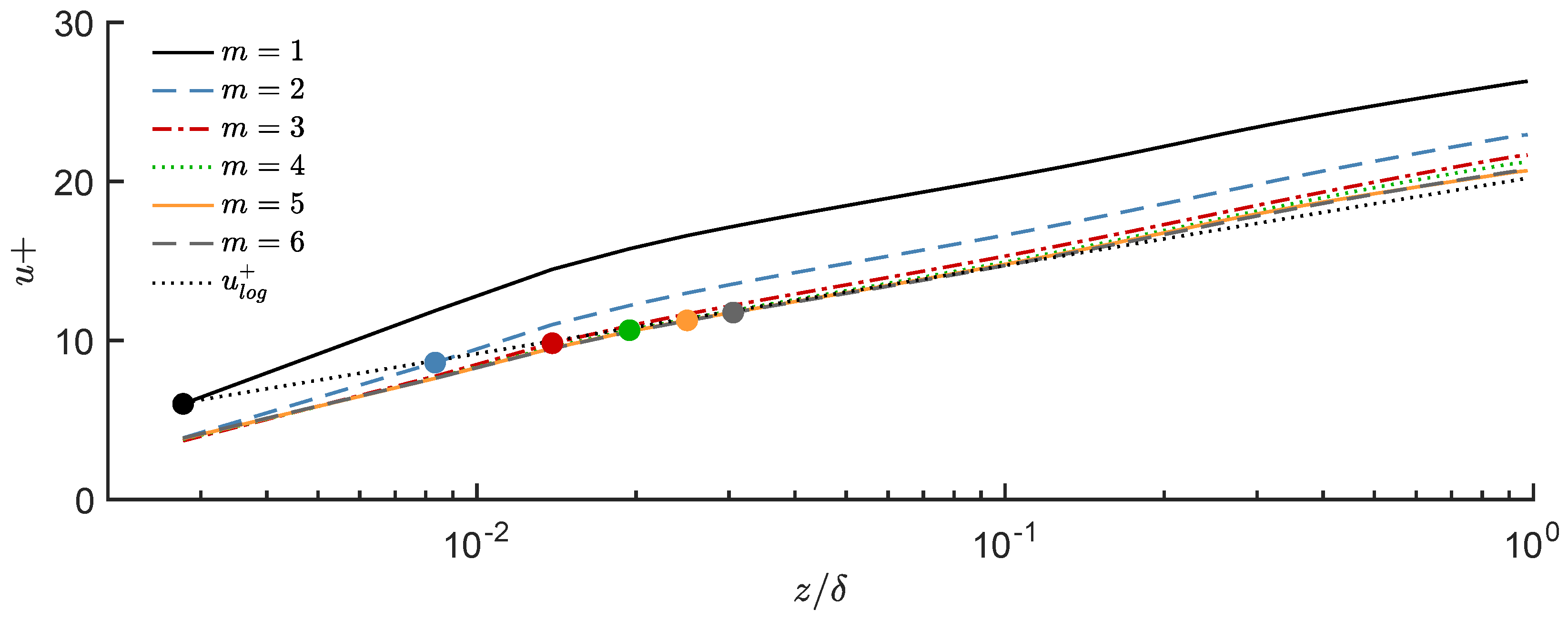
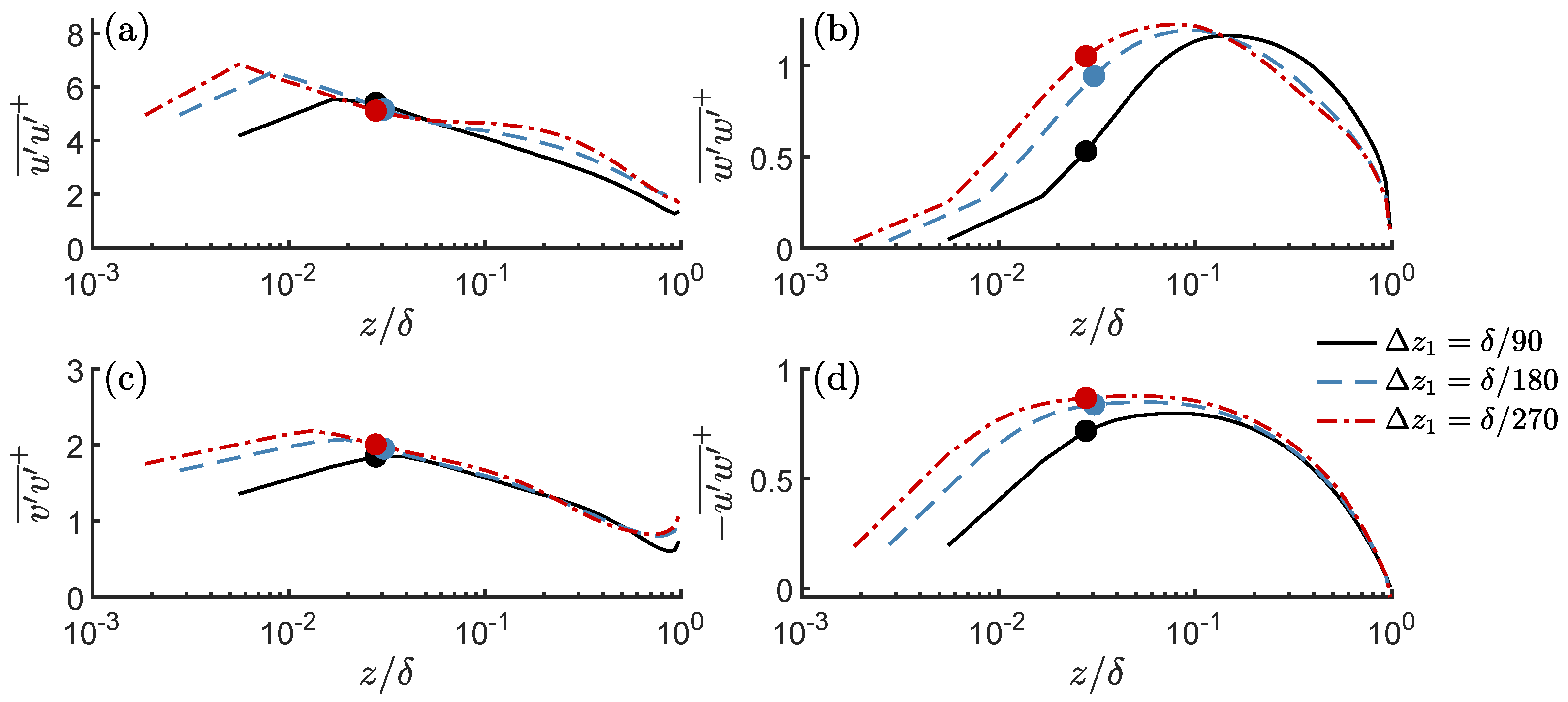
2.2.3. Grid Resolution Sensitivity

Another sensitivity study was carried out with respect to the grid resolution. No strict guidelines are available concerning the minimum grid resolutions for LES with wall-models. Piomelli et al. (2008) [62] report that grid-independent values for Reynolds stresses in the outer part of the boundary layer can not be reached for mesh spacings $\Delta >\delta /15$, since integral scales of turbulence have to be resolved by LES, independent of the particular wall-stress modeling approach. Davidson [63] suggests minimum resolution requirements based on the analysis of two point correlation. Furthermore, studies with high Reynolds number flows along smooth walls indicate that the scales of the most energetic resolved near-wall eddies are not independent of the chosen mesh resolution, leading to the emergence of so-called “super-streaks” [64]. These criteria and observations are likely to apply to LES of flow over rough walls too, since within the wall-stress model approach the only difference between smooth and rough walls is the numerical value of $u^{+}\left(z_m\right)$ in the relation (4).

The grid sensitivity was tested for three resolutions $\Delta z/\delta =0.01, 0.0055$ and 0.0038, corresponding to axial spacings $\Delta x/\delta =0.09, 0.044$ and 0.03 since the aspect ratio $\Delta x/\Delta z=8$ was kept the same. The lateral spacing was set to $\Delta y=0.5\Delta x$. The roughness length is set to $\delta /z_0=4500$ and the off-wall position is selected as $z_m/\delta \approx 0.03\delta$, corresponding to $m=3,6,8$ on the three different meshes.

Whereas profiles of the mean axial velocity show little influence of the grid resolution, we observe differences in the wall-normal turbulence intensity profiles, shown in Figure 3. Approximate grid independence is found when the resolution satisfies $\Delta x/\delta \le 0.044$, $\Delta y/\delta \le 0.022$ and $\Delta z/\delta \le 0.0055$. More details are reported in [14] where the influence of the cell aspect ratio is also documented.

Overall, these findings confirm the above-mentioned resolution criteria of Piomelli [62]. We have shown that consistent profiles of mean flow and Reynolds stresses are obtained for the outer layer of a boundary layer over a wall with moderate roughness with the standard wall-stress model as long as the evaluation point $z_m$ is located sufficiently off the wall. The wall-stress models serve the primary goal to guarantee a correct relation between $u_{\tau }$ and $\overline{u}\left(z\right)$ and correct levels of turbulence fluctuations at positions $z\ge z_m$. Our results demonstrate that the standard wall-modeling approach does not allow to extract reliable information on near-wall properties of turbulent fluctuations. However, it is likely to model correctly the interaction of the boundary layer turbulence with the wake of a wind turbine as long as the lowest blade tip position falls sufficiently above the location $z_m$.

2.2.4. Virtually Lifted-Wall Stress Model

The grid resolution for the study of the wake evolution by LES is driven by the need to adequately resolve the thin shear layers emanating from the blade tips. Thus, the grid resolution might be smaller than that which would be chosen if only the boundary layer evolution along a plate would be simulated. As a consequence, for large roughness $z_0$ the wall-normal width $\Delta z_1$ of the first wall-adjacent cell might reach the order of the roughness length $z_0$. This was found to cause stability problems in our solver INCA when the standard wall-model was used.

Saito et al. [65] developed a virtually lifted wall model for sub-grid roughness where it is assumed that the lower boundary of the computational domain is lifted into the overlap region where the total shear stress can be considered as constant and where the logarithmic law can be applied. Similarly, we developed a heuristic wall model that makes use of a lifted boundary to obtain a wall-stress formulation applicable to small $\Delta z_1/z_0$ ratios. In the spirit of the smooth-wall approach of Flores & Jiménez [66], wall-normal velocity disturbances are prescribed that are derived from integrating the continuity equation from the ground up to the the new permeable domain boundary which is lifted by the roughness length $z_0$ above the ground. There, the logarithmic law for rough walls predicts a zero-mean axial velocity. Other than in Saito et al. [65], the magnitude of the wall-normal fluctuations is determined from a control law that ensures that the axial mean flow in the first cell takes a positive value bounded by the logarithmic law. Full details of the implementation are described in [14].

A systematic study has been carried for a fixed mesh spacing $\Delta z=\delta /180$ where the relative roughness length was varied as $\delta /z_0=4500$, 450, 180, and 90, corresponding to ratios of grid size to roughness in the range $\Delta z_1/z_0=25$, $2.5$, $1.0$, and $0.5$. Thus, the roughness length gradually exceeds the grid spacing. It was found that both wall models result in similar axial velocity distributions for small relative roughness lengths, e.g., $\Delta z_1/z_0\ge 2.5$. However, they depart for values below this threshold where the $u^{+}$ values of the standard model fall below the corresponding logarithmic law. Whereas profiles of the shear stress $\overline{u^{\prime }{w}^{\prime }}/u_{\tau }^2\left(z\right)$ showed little influence on the wall-model type and on the ratio $\Delta z_1/z_0$, the new lifted-wall model produced high levels of the intensities $\overline{u^{\prime }{u}^{\prime }}$ and $\overline{v^{\prime }{v}^{\prime }}$. Intensity levels in the outer part of the boundary layer were not affected [14].

Overall, the lifted-wall model can be regarded a suitable alternative to the standard wall-stress model in order to obtain a stable solution that exhibits a correct ratio of $u_{\tau }/u\left(z_h\right)$, a logarithmic mean flow profile and realistic intensity levels in those parts of the boundary layer that interact with the rotor wake.

2.3. Actuator Line Modeling of the Rotor

For the primary interest of this study, namely, the evolution of the rotor wake over a distance of several rotor diameters, it is not necessary to resolve the flow over the blades in detail as long as the main flow structures such as tip vortices are reproduced with sufficient accuracy. Therefore, we employ the actuator line method (ALM) in order to model the flow resistance and the power extracted by the rotor.

The implementation of the ALM in INCA follows closely the reformulation for primitive variables by Mikkelsen [21]. The method consists in the enforcement of a time-dependent, distributed volume forcing in the rotor plane. Rotor blades are divided into radial segments on which their contribution to thrust and torque are computed from tabulated lift and drag coefficients $C_L\left(\theta \right)$ and $C_D\left(\theta \right)$ as function of angle of attack $\theta$ and of the local value of the relative wind speed. The momentum balances are then solved with incorporation of spatially smeared, rotating azimuthal and axial volume forces representing the blade loading. Concerning the radial number of actuator points and parameters of the regularization kernel used for smoothing the volume forcing we followed the recommendations of Mikkelsen [21] and Tossas [33].

The implementation has been validated for the 5 MW reference wind turbine designed by the National Renewable Energy Laboratory. Excellent agreement with results from EllipSys3D [45] is found for a case with steady inflow, both for the predicted blade polars and the flow field downstream of the rotor. Details are reported in [14].

2.4. Blade Polar Identification

The rotating body forces introduced by the actuator line method primarily depend on the tabulated airfoil data. Since the body forces determine the flow field evolution in the wind turbines wake, the quality of the tabulated airfoil parameters is crucial for an accurate modeling. In the design process of the model wind turbine, described in detail in [14], airfoil data obtained by solving two-dimensional boundary layer equations for blade segments was used. These computations do not take into account any rotational or three-dimensional effects, nor the finite length of the blades and the formation of tip vortices. As a consequence, the measured and the predicted performance of the model rotor exhibited significant deviations.

In order to obtain good quantitative agreement of measured thrust T and torque Q respectively extracted power $P=\mathsf{\Omega }Q$ in dimensionless form

$$C_T=\frac{T}{\frac{1}{2}\rho {\overline{u}}_h^2\pi R^2},C_P=\frac{P}{\frac{1}{2}\rho {\overline{u}}_h^3\pi R^2},$$

(6)

with the outcome of the ALM modeling of the rotor, blade polars were calibrated using a 3D-RANS simulation-based approach as in [67,68].

In our approach, the Blade Element Momentum (BEM) theory [69,70] is inverted. In summary, the axial and tangential induction factors are determined iteratively from the blade forces deduced from 3D RANS simulations. These are then used to calculate the angle of attack as well as the lift and drag characteristics of a rotor blade. Including Prandtl’s tip loss correction and Glauert’s correction for large induction factors, the inverse BEM method has been implemented as described in [67], see [14] for details.

To obtain lift and drag coefficients over a broad range of angles of attack with sufficient resolution, blade forces for different tip speed ratios and blade pitch angles have to be computed. For this purpose the fully compressible viscous steady state RANS solver CFX by ANSYS Inc. is applied. In order to reduce the computational costs only a 120${}^{\circ }$ segment of the wind turbine is simulated and the presence of the tower is neglected. Rotational forces are considered by simulating in a rotating frame of reference. Periodic boundary conditions are prescribed in the circumferential direction.

Distributing 15 cells across the boundary layers on the blades and maintaining a near-wall resolution of $y_{ave}^{+}=0.88$ the computational domain was discretized into 10 million cells. Assuming transition on the blade surfaces to occur very early the two-equation $k-\omega$ shear stress transport (SST) model was used everywhere. The rotational frequency of the rotating domains and the freestream velocity at the inlet were chosen such to arrive at an average chord based Reynolds number of ${\overline{Re}}_c=$ 62,500. Numerical simulations have been carried out for blade pitch angles ${\mathsf{\Theta }}_p=-2^{\circ }$ to $6^{\circ }$ with an increment of $\Delta {\mathsf{\Theta }}_p=1^{\circ }$. For each pitch angle the tip speed ratio $\lambda =\mathsf{\Omega }R/\overline{u}\left(z_h\right)$ was varied from $\lambda =2$ to 12 with an increment of $\Delta \lambda =0.5$.

To verify the accuracy of the simulation results, Figure 4 shows the power and thrust coefficient as function of the tip speed ratio for pitch angles of ${\mathsf{\Theta }}_p=0^{\circ },1^{\circ },2^{\circ }$ obtained from the 3D blade-resolving simulation (RANS), and compares them with the results of the wind tunnel measurements (EXP) and the values predicted initially in the design process of the blades (DSGN).

Most salient in the comparison of the thrust coefficients in Figure 4a–c is the good agreement of the RANS simulation and measurement data in comparison to the values predicted in the design process, whereas the comparison of the obtained power coefficients shown in Figure 4d–f shows no significant improvement by the RANS simulation.

Figure 5 shows lift and drag polars based on the blade forces of the three-dimensional RANS simulation and derived by the inverse BEM method. These are compared to the airfoil characteristic used in the design process (DSGN) where no radial dependency of the airfoil characteristics is considered which turns out to be a crude approximation. Characteristics of the inverse BEM method based on the RANS results for different positions $\mu =r/R$ show a significant radial dependency of the lift and drag characteristics due to rotational and three-dimensional effects: (i) Lift values are reduced for all AoA $\theta$ along the complete span of the blade, which is even more significant at the blade tip due to the presence of the strong blade tip vortices there; (ii) Drag values for low AoA are similar in the middle of the blade span, whereas they are increased for high AoA and at the outer sections of the blade.

According to the BEM Theory, the generation of thrust is mainly dominated by the lift coefficient. Hence, it is consistent that similar lift characteristics result in similar thrust coefficients as it is the case for the design and the calibrated airfoil characteristic. The generally lower lift coefficient and its radial dependency predicted by the inverse BEM method is the main reason for the very good agreement of $C_P$ and $C_T$ with the measurement results. The argumentation for the connection of power coefficient and airfoil characteristic is more complex as the generation of torque is not solely dominated by the lift but by the drag coefficient as well. See [14] for a detailed discussion.

The thrust of the rotor determines the velocity deficit in the wake of the wind turbine. Therefore, the airfoil characteristics obtained with the inverse BEM method based on the 3D-RANS simulation that predict the thrust with high accuracy, will be used as input for the ALM blade modeling in our LES.

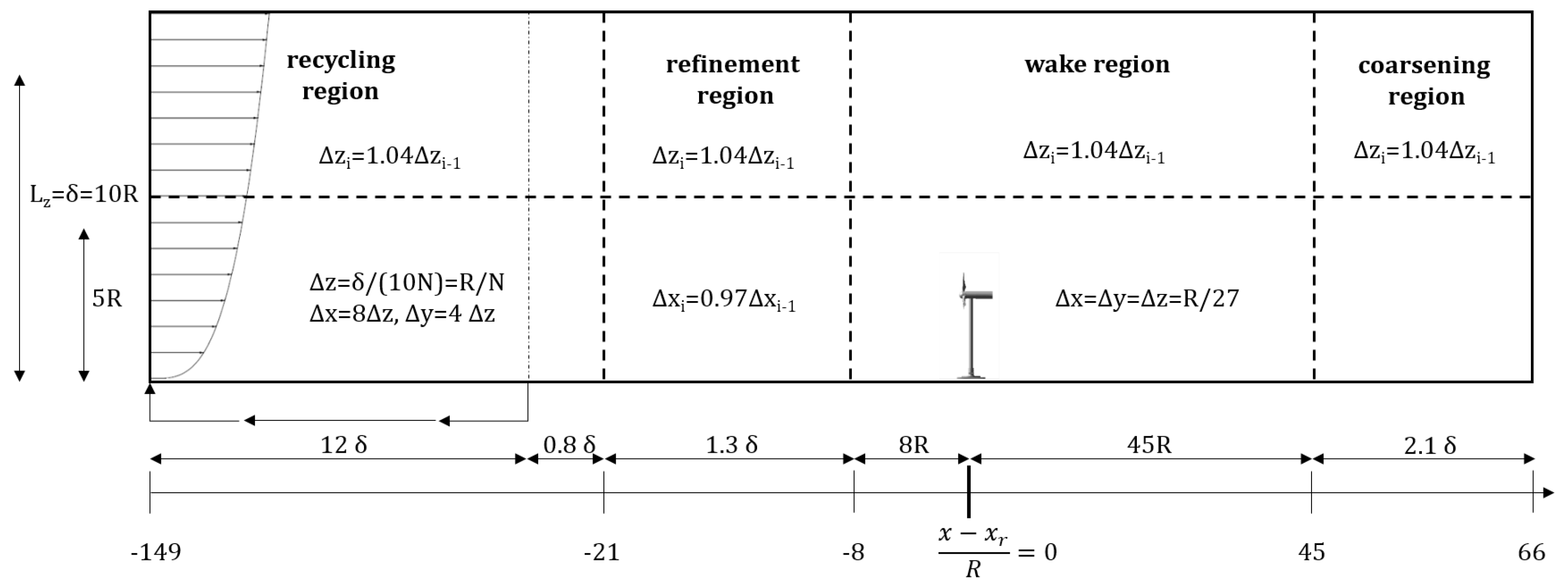
2.5. Set-Up of the Full LES Simulation

In Figure 6, a draft of the computational domain for the wind turbine wake simulation is shown. The domain height is set equal to the boundary layer height of $L_z=\delta =10R=$ 2250 mm. This choice was found to yield the best agreement of boundary layer parameters at hub height $z_h=2R$ with the reference wind tunnel data. Lateral width and axial extent are $L_y=4\delta$ and $L_x=21.6\delta$. To reduce the computational costs the domain is divided at half height in a lower and an upper part. In the lower part where the wake evolution takes place, the wall-normal spacing of $\Delta z=R/N$ is kept constant, whereas it is gradually increased as $\Delta z_i=1.04\Delta z_{i-1}$ in the outer part.

In axial direction the computational domain is sub-divided into four regions. The 1st region is the so-called recycling region in which a turbulent flow with a desired boundary layer profile is generated. At a distance of $12\delta$ downstream of the inlet plane a “recycling” plane is defined where unsteady flow data are extracted to be fed in again at the inlet. In order to reduce the computational costs the recycling region exhibits a coarser grid resolution in the axial and lateral direction as the wake region where the wind turbine and its wake are located. Cell aspect ratios of $\Delta x/\Delta z=8$ and $\Delta y/\Delta x=0.5$ are chosen there.

A refinement region is introduced that connects the recycling region with the wake region. There, the grid is first gradually refined in the axial direction with a grid spacing of $\Delta x_i=0.97\Delta x_{i-1}$ starting from a resolution of $\Delta x=8R/N$ in the recycling region down to a resolution of $\Delta x=R/N$. This is then followed by a step-wise refinement of the lateral resolution from $\Delta y=4R/N$ to $\Delta y=2R/N$.

The 3rd region is the so-called wake region with a total length of $53R$. It is subdivided in a middle part with a width of $8R$ and cubic cells of $\Delta x=\Delta y=\Delta z=R/N$ and two neighboring lateral parts where the grid is gradually coarsened. Within the middle part the wind turbine is located $8R$ downstream of the beginning of this region, which leaves another $45R$ equidistant region within which the wake development is captured. The wake region is then followed by the so-called coarsening region where the grid is gradually coarsened towards the outlet. For our baseline resolution of $N=27$ points per rotor radius ($\Delta z=\delta /270$) the domain is discretized in 92 million cells which are distributed over 1344 blocks.

2.5.1. Boundary Conditions

At the domain inlet unsteady velocity values are prescribed that are obtained from an internal-mapping approach. During each time-step the instantaneous velocity field at the recycling plane $u_{i,rec}(y,z)$ is recorded. In order to avoid any upstream influence from the blocking of the wind turbine on the approaching flow time averages ${\overline{u}}_{i,rec}(y,z)$ and ${\overline{{u_i^{\prime }}^2}}_{rec}(y,z)$ of the recycled flow field are computed. The flow field is then rescaled such that the mean flow at the inlet equals a prescribed mean flow ${\overline{u}}_{i,in}(y,z)={\overline{u}}_{i,target}\left(z\right)$ that is derived from a half-channel simulation with axially periodic boundary conditions. In order to maintain a desired axial mean velocity at hub height $z_h$, a further scaling is required, yielding the final rescaling procedure as

$$u_{i,in}(y,z)={\overline{u}}_{i,target}\left(z\right)+\sqrt{\frac{{\overline{{u_i^{\prime }}^2}}_{target}\left(z\right)}{{\overline{{u_i^{\prime }}^2}}_{rec}(y,z)}}·(u_{i,rec}(y,z)-{\overline{u}}_{i,rec}(y,z)).$$

(7)

At the domain outlet the convective boundary condition $\frac{\partial u_i}{\partial t}+{\overline{u}}_{target}\left(z\right)\frac{\partial u_i}{\partial x}=0$ is set. Along the ground either the standard wall-stress model or the lifted wall model for the case with large roughness $z_0$ is used. At the top boundary, a free-slip condition is prescribed with the consequence that a weak axial mean pressure gradient is imposed in the computational domain. The lateral boundary conditions are chosen to be periodic.

2.5.2. Parameters of Investigated Cases

For validation of the LES approach wind-tunnel measurements of wake evolution over homogeneous roughness are available for two roughness scales $z_0$.

Table 1. Characteristics of the turbulent boundary layers in the reference experiment [15].

Name	Acronym	${\mathit{z}}_0$ [mm]	$\mathit{\alpha }$	${\mathit{u}}_{\mathit{\tau }}$ [m/s]	${\mathit{I}}_{\mathit{u}}\left({\mathit{z}}_{\mathit{h}}\right)$	${\mathit{z}}_0^{+}={\mathit{u}}_{\mathit{\tau }}{\mathit{z}}_0/\mathit{\nu }$
SBL	sf016	0.51	0.16	0.65	8.3%	19
RBL	sf032	5.06	0.32	0.89	13.8%	190

summarizes the properties of the two cases named smooth boundary layer (SBL) and rough boundary layer (RBL) characterized by shear exponents $\alpha =0.16$ (SBL) and $\alpha =0.32$ (RBL). The turbulent inflow differs strongly with respect to shear exponent and turbulence level $I_u=u_{rms}/{\overline{u}}_{bl}$ at hub height $z_h$, representing a neutrally stratified atmosphere over rural and forested terrain at a scale of 1:$\mathcal{O}\left(350\right)$ extending vertically over 525 m. The model scale was chosen to assure Reynolds number independence of the main flow statistics and a realistic rotor performance. For all investigated cases $z_0^{+}$ exceed the threshold 2.8 for the fully rough regime [14,61]. The Reynolds number based on the rotor diameter $R{e}_D={\overline{u}}_{bl}\left(z_h\right)D/\nu =3.04\times {10}^5$ exceeds the lower limit established by Chamorro et al. [71] for the wake flow to become independent of Reynolds number.

As part of the recycling procedure for the generation of turbulent inflow, the mean axial flow at hub height is maintained at the reference speed ${\overline{u}}_h\equiv {\overline{u}}_{bl}\left(z_h\right)=10.8\mathrm{m}/\mathrm{s}$ in all cases considered. The angular velocity of the turbine is selected such that the tip-speed ratio reaches $\lambda =\mathsf{\Omega }R/{\overline{u}}_h=6.5$ where the maximum power was extracted by the model in the wind-tunnel experiment. The rotor of the wind turbine is modeled by 36 uniformly distributed actuator points per blade. The regularization parameter of the actuator line method is set to $ϵ=3\Delta x$. Blade polars determined by the inverse BEM-approach for a pitch angle of ${\mathsf{\Theta }}_p=1^{\circ }$ are used subsequently.

Measurements and simulations were carried out for different yaw angles in the range $-{30}^{\circ }\le \gamma \le {30}^{\circ }$. Here we focus on the results for zero yaw angle $\gamma =0^{\circ }$. The yaw angle influence is discussed in detail in [14]. The grid sensitivity was studied for case SBL by comparing results from the baseline resolution $N=27$ ($\Delta z/\delta =270$) with a coarser mesh with $N=18$.

Simulations proceeded in three stages, including generation of a turbulent boundary layer in the empty domain, followed by activation of the ALM approach to simulate the turbine. After a transient of 400 rotor revolutions the wake is fully developed and flow statistics such as mean flow ${\overline{u}}_i$ and Reynolds stresses $\overline{u_i^{\prime }{u}_j^{\prime }}$ are collected. To distinguish LES cases we use the acronyms sf016 and sf032.

3. Comparison of LES Results with Measurements

3.1. Flow Evolution in the Empty Domain

Since the computational domain consists of regions with different grid resolution, the flow quantities undergo transients in the axial direction. This is an unavoidable property of LES since the ratio of integral scale of the turbulence to the length scale of the grid cut-off affects the evolution of the resolved scales [63,64]. Here we quantify this effect in the current simulations.

Figure 7 shows (a) the mean axial velocity $\overline{u}(x,z_h)$ and (b) the turbulent kinetic energy $K(x,z_h)$, both at hub height $z_h$ in the empty domain without the turbine. For the baseline resolution of $N=27$ both quantities vary in axial direction. Some transients are triggered by the rescaling procedure applied at the inlet. After the flow has settled in the recycling region, new transients appear both in the refinement and in the wake region. These are induced by the changes in grid resolution.

The axial changes are more pronounced for the high roughness ($\alpha =0.32$) case. Within the wake region 0 < x < 24R the axial variation at hub height is less than 2% for the mean axial flow, but up to ≈15% for the kinetic energy of the large roughness. For intermediate roughness ($\alpha =0.16$) the TKE changes by less than $5\%$ in the same interval. This inherent gradual change of the background flow has to be kept in mind when assessing the wake evolution. However, since the rotor imposes a massive disturbance on the flow, the effects from the change in grid resolution do not seem to have a large impact on the wake behavior.

In order to discuss the effect of the grid refinement between the recycling region and wake region on the axial flow evolution in more detail, Figure 8 shows vertical profiles at selected axial positions within the wake region ($-4<(x-x_r)/R<20$) for the mean axial velocity $\overline{u}$, the axial intensity $\overline{u^{\prime }{u}^{\prime }}$, the Reynolds shear stress $\overline{u^{\prime }{w}^{\prime }}$ and the turbulent kinetic energy K, all normalized with respect to ${\overline{u}}_h=\overline{u}(x_r,z_h)$. Experimental data of the SBL and RBL configurations are included.

Figure 8a,e show that the velocity profiles $\overline{u}\left(z\right)$ vary indiscernible within the wake region. On the other hand, the normalized profiles of the Reynolds stresses are significantly affected by the grid refinement. Thereby, it is interesting to notice that the change of the axial intensity $\overline{u^{\prime }{u}^{\prime }}$ increases for higher roughness $z_0$, Figure 8b,f. The same holds for the lateral intensity $\overline{v^{\prime }{v}^{\prime }}$.

Comparison of axial intensities in case sf016 ($\alpha =0.16$) for different values of N resp. $\Delta z/\delta$ show larger axial changes for $N=18$ than for $N=27$. This can be interpreted as underresolving the inertial subrange in the recycling region and will be discussed in more detail further below.

For intermediate roughness $\alpha =0.16$ the agreement of simulation and measurements is very good in the wake region despite the slight axial variation of the Reynolds stress profiles. For higher roughness $\alpha =0.32$, the match of profiles from simulation and experiment is less satisfactory. Still, mean shear and Reynolds stress levels are comparable in the region $z_h-R<z<z_h+R$ where most of the wake evolution takes place. A likely reason for the mismatch is the fact that the boundary layer in the wind tunnel has not developed axially over a long fetch, reaching equilibrium [53]. Thus, a better match might be obtained when the entire process of boundary layer generation in the wind tunnel with a combination of castellated barriers and vertical fins is included in the simulation.

Figure 9 shows the normalized spectral density for the three velocity components as function of the wave length k, which is obtained by Taylor’s frozen turbulence assumption as $k=2\pi f/\overline{u}\left(z_h\right)$. Simulation results for $\alpha =0.16$ at two axial positions and for two resolutions N are compared to measurements in the empty wind tunnel. The two axial positions include the recycling region and the wake region. Spectra from the simulation match measurements over a considerable range of scales, including parts of the inertial subrange, in the wake region. Conversely, spectra from the recycling region agree less with the experiment. Due to the coarser resolution the inertial range is hardly resolved and spectral densities are too high at wavenumbers above the grid cut-off.

Whereas the prediction is generally improved for the grid resolution of $N=27$, the energy cascade is still not captured correctly within the recycling region. Rather, when transported into the well-resolved wake region, the turbulence scales start to reorganize, which manifests itself in the gradual axial development of the Reynolds stress tensor components as shown in Figure 8. As the energy cascade within the recycling region is better resolved for $N=27$ than for $N=18$, the reorganization of turbulent scales in this case is reduced within the wake region; see Figure 8f–h.

Overall, the chosen approach employing zones with different grid resolutions appears to be a good compromise since a good match with measured turbulence properties is achieved in the wake region without having to spend excessive computational resources in the recycling region for the generation of turbulent inflow data.

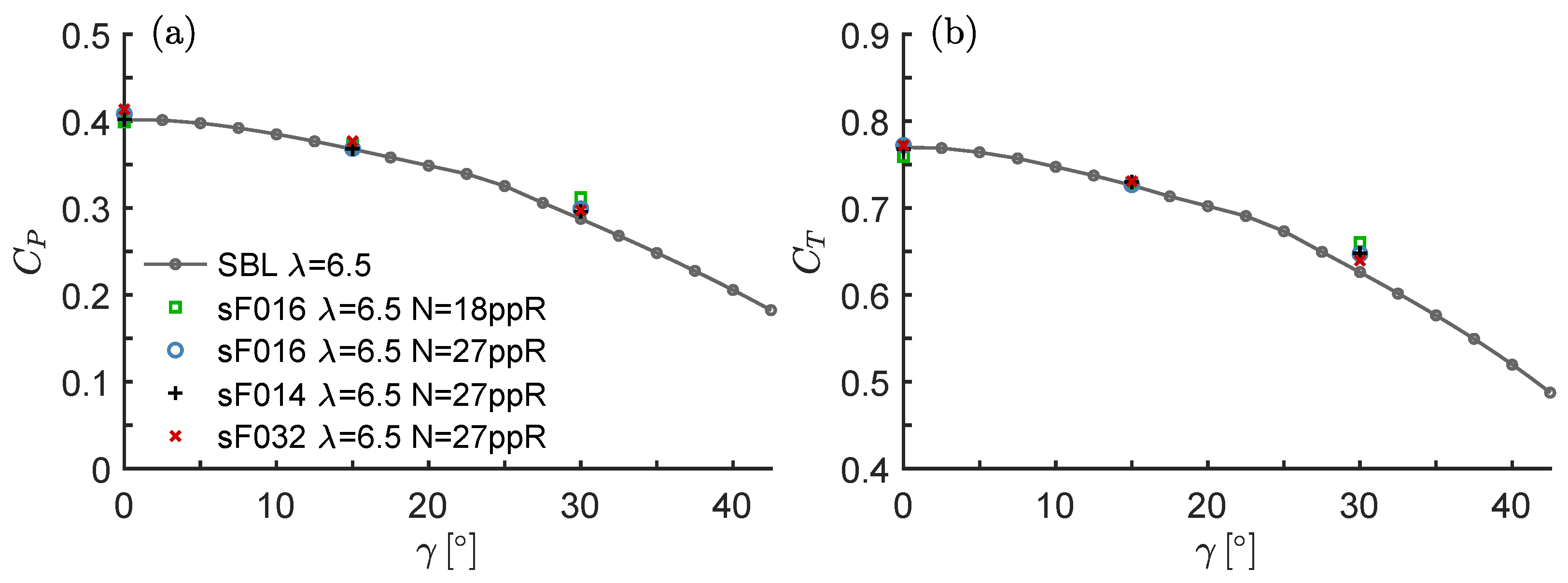
3.2. Rotor Performance

Since the ”calibration” of lift and drag polars through the inverse BEM method was carried out with 3D-blade resolving RANS data, it is not guaranteed that performance data from the ALM implementation in the LES model will agree with the wind-tunnel measurements. Figure 10 shows the power and thrust coefficient as function of the yaw angle for the medium roughness simulation case sF016 ($\alpha =0.16$) with grid resolutions of $N=18$ and $N=27$ ppR. In addition, coefficients from LES simulations with smaller ($\alpha =0.14$) and higher roughness ($\alpha =0.32$) are shown as well. Measurements are included for $\alpha =0.16$ only, since thrust and power coefficients for $\alpha =0.32$ are nearly identical. The graph shows that for a given yaw angle all numerical configurations yield similar coefficients, which are in very good agreement with the experimental results. The deviation from experiment of the rotor performance predicted by the simulations with grid resolutions of $N=27$ ppR is <4% for the power coefficient and <3% for the thrust coefficients. The small differences in between the cases with different roughness length is to be expected as the same holds for the experimental results as documented in [14,53].

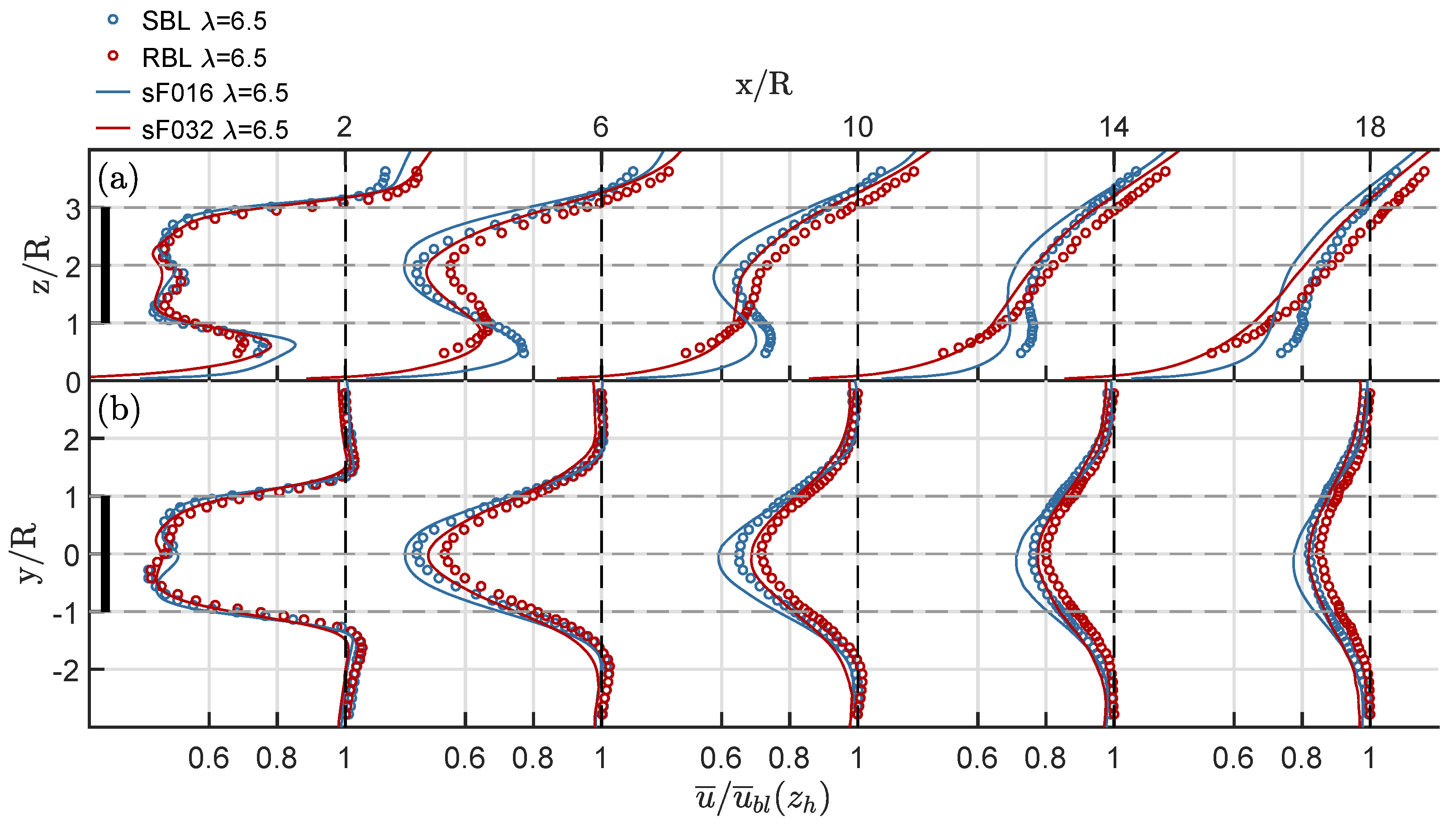
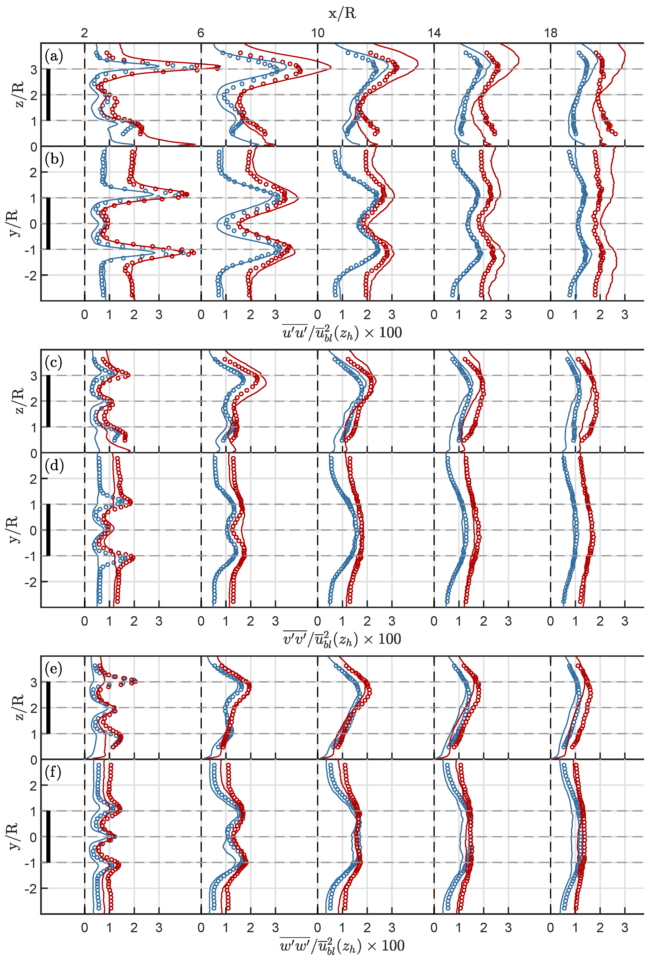
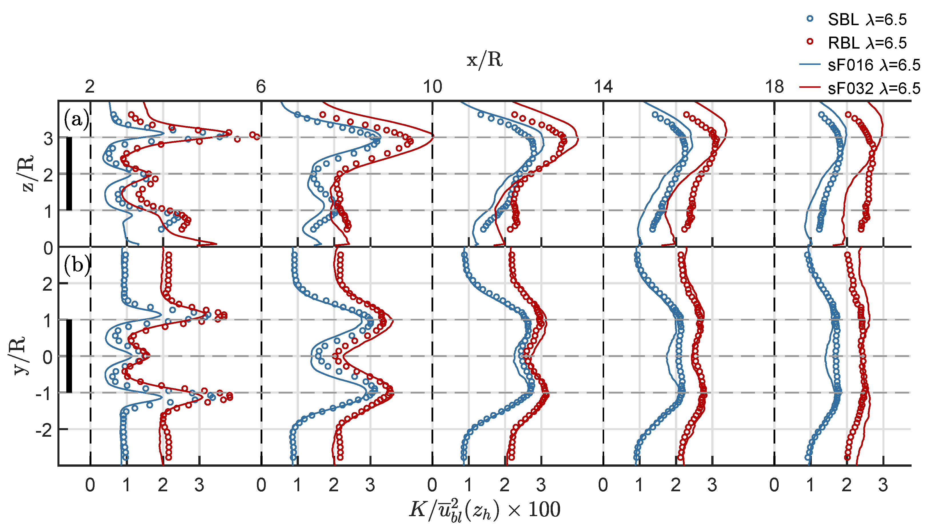
3.3. Flow Field in the Wake Region

Now we are ready to assess the flow field evolution downstream of the rotor. First, vertical and lateral profiles of mean flow, turbulence intensities and Reynolds shear stresses will be compared. Thereafter, integral parameters of the wake are shown. For the validation we focus on the wake evolution for zero yaw angle $\gamma =0^{\circ }$. Results are shown for grid resolutions $N=27$ resp. $\Delta z/\delta =1/270$. For case sf016 ($\alpha =0.16$) the grid sensitivity has been investigated by comparing results with $N=27$ and $N=18$, see [14].

Figure 11 shows the spatial distribution of the normalized mean axial velocity component $\overline{u}/{\overline{u}}_{bl}\left(z_h\right)$ in (a) the mid-vertical and (b) the mid-horizontal plane. Shortly behind the rotor disk at $x/R=2$, mean flow profiles match closely except below hub height in the vertical cut plane. There, the higher velocities in the LES for $z<R$ are likely a result from neglecting the tower in the simulation. Further downstream, simulated and measured profiles maintain fairly similar shapes for both roughness values. However, the LES shows a slightly deeper wake and a nearly constant offset in the vertical plane when compared with the measurements.

We do not have a straightforward explanation for the cause of this mismatch. Since these differences are of the same order for both roughness values, they do not seem to originate from a mismatch of the upstream flow condition which was more prominent for $\alpha =0.32$ than for $\alpha =0.16$. The slightly deeper wake center in the simulation might partially be caused by neglecting the nacelle.

Simulations and experiment agree very well with respect to the change rates of profile shapes as the wake develops downstream. Furthermore, the LES captures the quantitative difference in the wake evolution associated with the change in roughness very well, making this simulation approach a valuable tool for detailed analysis of the underlying flow physics, e.g., by assessment of the budgets for momentum and for turbulent kinetic energy; see [14].

The mean flow profile shape is closely connected with the spatial distribution of Reynolds shear stresses since their gradients dominate the momentum budget in regions with strong shear as in the shear layer emanating from the rotor edge. Figure 12 shows the spatial distribution of the shear stress (a) $\overline{u^{\prime }{w}^{\prime }}$ in the mid-vertical and (b) $\overline{u^{\prime }{v}^{\prime }}$ the mid-horizontal plane, both normalized with the hub height mean velocity ${\overline{u}}_h^2$ of the undisturbed boundary layer.

In general the shear stress is well predicted by the simulations. Whereas for case SBL the maxima in the computed shear stress magnitudes are somewhat underpredicted in the near wake ($x/R=2$), they reach similar levels as the experiment for case RBL. Presumably this is related to some deficiencies of the ALM modeling of the rotor by smeared body forces. As shown later, turbulence intensities near the rotor tips in the near wake are not well predicted with the ALM model.

A feature that is well reproduced by the LES is the shift of the $\overline{u^{\prime }{w}^{\prime }}\left(z\right)$-profiles to more negative values with increasing roughness $z_0$ which is a result of the higher magnitude of the (negative) background shear stresses in case RBL on which the wake is ‘superimposed’.

The change in roughness has hardly any influence on the lateral shear stress profiles $\overline{u^{\prime }{v}^{\prime }}\left(y\right)$. Still, the shape of the lateral profile of axial mean flow, $\overline{u}(y,z_h)$, and the lateral wake width ${\sigma }_y$ (shown below) differ considerably for cases SBL and RBL. Co-spectra $C{o}_{u^{\prime }{v}^{\prime }}\left(f_h\right)$ recorded at lateral position $y\approx \pm R$ of maximum shear stress magnitudes (not shown here, see [14]) show that lateral shear stresses are carried by the same scales for both roughness values. In both cases, the maximum of the (co)spectral density in the medium to far wake is centered around a frequency $f=Sr\overline{u}\left(z_h\right)/\left(2R\right)$ with $Sr\approx 0.2$ as would be expected for a bluff body of diameter $2R$ immersed in a uniform stream $\overline{u}\left(z_h\right)$. For the particular situation with $\lambda =6.5$, this corresponds to 1/10 th of the rotor shaft frequency.

Profiles of turbulence intensities (the diagonal Reynolds stress tensor components) $\overline{u^{\prime }{u}^{\prime }},\overline{v^{\prime }{v}^{\prime }},\overline{w^{\prime }{w}^{\prime }}$ are shown in Figure 13. We observe a good qualitative agreement of Reynolds stress profile shapes in the vertical cut plane and good quantitative agreement in the horizontal plane except for the near-wake position $x=2R$. There, peak values of $\overline{v^{\prime }{v}^{\prime }}$ and $\overline{w^{\prime }{w}^{\prime }}$ are significantly lower in the LES than in the measurements. The agreement is better for the axial intensity $\overline{u^{\prime }{u}^{\prime }}$ with a better match for case RBL than for case SBL. The deviations of the LES results from measurements in the near wake are likely caused by the limitations of the ALM approach that is not capable to correctly reproduce all flow details in the blade tip region.

In the mid and far wake, deviations between measurements and LES are most prominent for the axial and lateral intensities and are slightly higher for case RBL than for case SBL. For the wall-normal intensity $\overline{w^{\prime }{w}^{\prime }}$ the agreement between simulation and experiment is the best and equivalent for cases SBL and RBL. Very close to the ground, the artificially high values of axial intensity in case RBL are associated with the lifted-wall modeling of the roughness. As seen for the Reynolds shear stresses, the lateral profiles of all three intensities in the horizontal cut plane agree much better than the vertical profiles. The only exception are the profiles of $\overline{u^{\prime }{u}^{\prime }}\left(y\right)$ for case RBL which show too high values in the LES for $x\ge 10$. The overprediction of axial intensity in case RBL is also clearly visible in the vertical profiles $\overline{u^{\prime }{u}^{\prime }}\left(z\right)$, starting at $x=6R$. This deviation might be associated with the gradual changes resulting from the adaption to different grid resolutions. In Figure 8b, a similar trend can be seen for case RBL in the empty flow domain.

As observed for the mean flow profiles, the LES captures quantitatively very well the relative changes in the turbulence intensity profiles associated with the change in roughness. Thus, derived quantities such as anisotropy parameters of the Reynolds stress tensor that might be of value in the development of fast wake prediction models might be deduced with some fidelity from this LES data base.

For completeness, profiles of the turbulent kinetic energy $K=0.5\rho \overline{u_i^{\prime }{u}_i^{\prime }}$ are shown in Figure 14. Since the axial component $\overline{u^{\prime }{u}^{\prime }}$ contributes most in such a strongly anisotropic shear flow, the TKE profiles show similar deviations as the previously discussed profiles of axial turbulence intensity. The sharp peaks in the proximity of the rotor are not well resolved by the simulations, perhaps due to the application of smeared body forces.

For most of the presented profiles of mean flow, intensities and Reynolds shear stresses the agreement between simulation and experiment is even better than shown here when the contribution of the undisturbed boundary layer, e.g., ${\overline{u}}_{bl}$ is subtracted out [14]. In [15], the concept of an ’added wake’ was brought forward, leading to the satisfactory collapse of normalized profiles when the wake contribution was isolated from the total by subtracting the boundary layer part. This technique might be helpful in the analysis of LES results from situation where inflow properties do not match perfectly as in the present case RBL.

Next, wake characteristics will be compared, including the wake center velocity deficit

$$\Delta u_C=max(\Delta u),\Delta u(x,y,z)=\frac{{\overline{u}}_{bl}\left(z\right)-\overline{u}(x,y,z)}{{\overline{u}}_{bl}\left(z\right)}$$

(8)

where ${\overline{u}}_{bl}\left(z\right)$ is the undisturbed boundary layer profile ahead of the turbine, the lateral and vertical wake widths ${\sigma }_y$ and ${\sigma }_z$, and the wake center position in the vertical direction $z_C$ derived from the velocity and momentum deficits according to

$${\sigma }_y=\frac{1}{\sqrt{2\pi }max(\Delta u)}{\int }_{-\infty }^{\infty }\Delta udy,{\sigma }_z=\frac{1}{\sqrt{2\pi }max(\Delta u)}{\int }_{-\infty }^{\infty }\Delta udz,z_C=\frac{{\int }_{-\infty }^{\infty }\Delta u^{2}zdz}{{\int }_{-\infty }^{\infty }\Delta u^{2}dz}.$$

(9)

Figure 15 shows the axial development of these parameters. The faster recovery of the wake with increasing background turbulence, and hence ground roughness, can well be observed in the centerline velocity deficit shown in Figure 15a. Despite the axial offset in the curves of $\Delta u$, the simulation and experiment agree very well with respect to the influence of roughness on the axial change rates of the wake deficit. Moreover, the evolution of the vertical wake center location shown in Figure 15d is very well reproduced in the simulation.

The comparison of the evolution of lateral and vertical wake width ${\sigma }_y$ and ${\sigma }_z$ in LES and experiment is hindered by the fact that these parameters are very sensitive with respect to small changes in profile shape. For example, the measurements of the lateral profiles $\overline{u}\left(y\right)$ shown in Figure 11 for case RBL show a slight asymmetry and an overshoot $\overline{u}\left(y\right)/{\overline{u}}_h>1$ at the edges of the wake which is not present in the LES.

Both for the lateral width ${\sigma }_y$ (Figure 15b) and the vertical width ${\sigma }_z$ (Figure 15c) the LES predicts considerably higher influence of ground roughness on the wake width as the measurements. Such a trend with increasing roughness would be consistent with the faster wake recovery, see [15]. However, an increase in wake width from case SBL to RBL is seen in the experiment only for ${\sigma }_z$, not for ${\sigma }_y$. Simulation and experiment agree slightly better with respect to the spreading rates in the far wake, predicting a nearly constant value of $d{\sigma }_i/dx$ in case SBL and and a non-linear behavior for $x/R>12$ for case RBL.

The deviations between LES and experiment seem to have several causes, including weaknesses of the ALM approach, a slight mismatch of the properties of the approach flow, subtle changes associated with the change in grid resolution, as well as neglecting the tower and nacelle in the simulation. Furthermore, the representation of the rough surface by a wall-stress model might not be sufficiently accurate in case RBL where the artificial roughness elements in the experiment have a size which corresponds to one-third of the distance between blade tip and ground. Thus, it is not easy to assess quantitatively the relative importance of the mentioned influence factors since it would require additional simulations where grid resolution, ALM parameters and ground modeling would have to be varied.

4. Summary and Conclusions

A high-fidelity numerical simulation approach is assessed with respect to its capability to quantitatively predict the influence of the roughness length $z_0$ of a neutrally stratified turbulent boundary layer on the evolution of the wake behind a horizontal-axis wind turbine. Wind tunnel measurements of the wake evolution behind a model wind turbine with rotor diameter $D=450\mathrm{mm}$ obtained for ground roughness $z_0=0.5\mathrm{mm}$ and $z_0=5\mathrm{mm}$, corresponding to shear exponents $\alpha =0.16$ and $\alpha =0.32$, with approach speed $\overline{u}\left(z_h\right)=10.8\mathrm{m}/\mathrm{s}$ are used as a reference. The numerical approach combines several modeling steps. For the first time, the implicit LES approach with approximate deconvolution developed by Hickel et al. [38] is combined with a wall-stress model to approximate the rough ground and an actuator line model (ALM) for representing the rotor blades. The main highlights, novel aspects and conclusions of this investigation are summarized as follows:

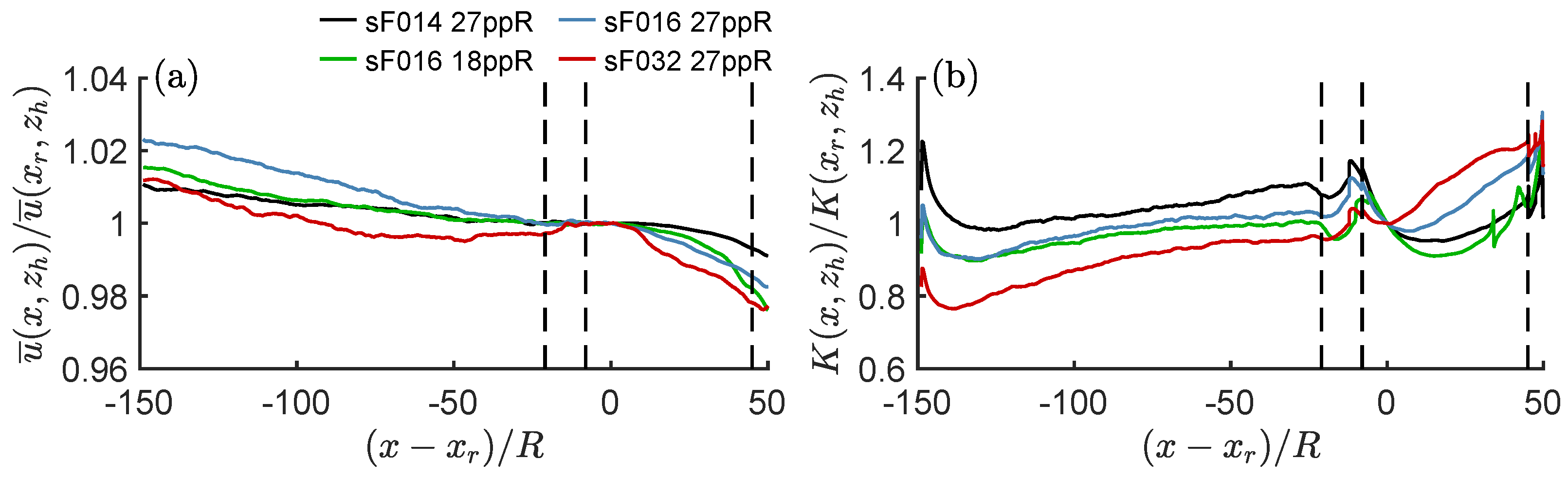
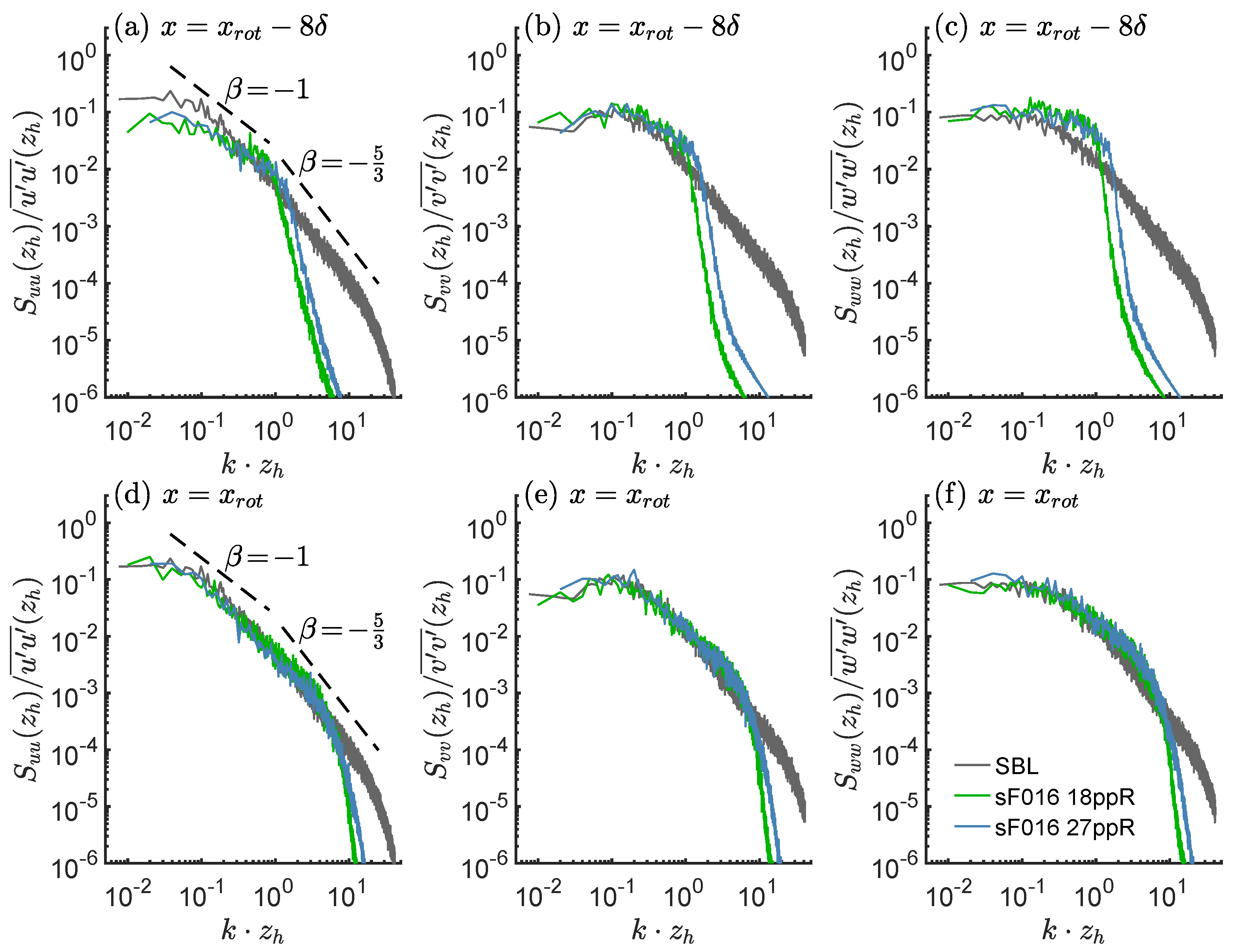
• In the fully coupled simulation approach, turbulent inflow is generated by an internal mapping approach (recycling technique) in an upstream segment of the computational domain with coarser grid resolution. Changes in the grid spacing significantly affect the axial evolution of turbulence intensities in case $\alpha =0.32$.
• The rough wall is approximated via a relation between instantaneous wall-shear stress and the tangential velocity at an off-wall position $z_m$. In accordance with [29], a better match with the logarithmic law of the wall is achieved when $z_m$ is chosen at least three cell layers away from the ground.
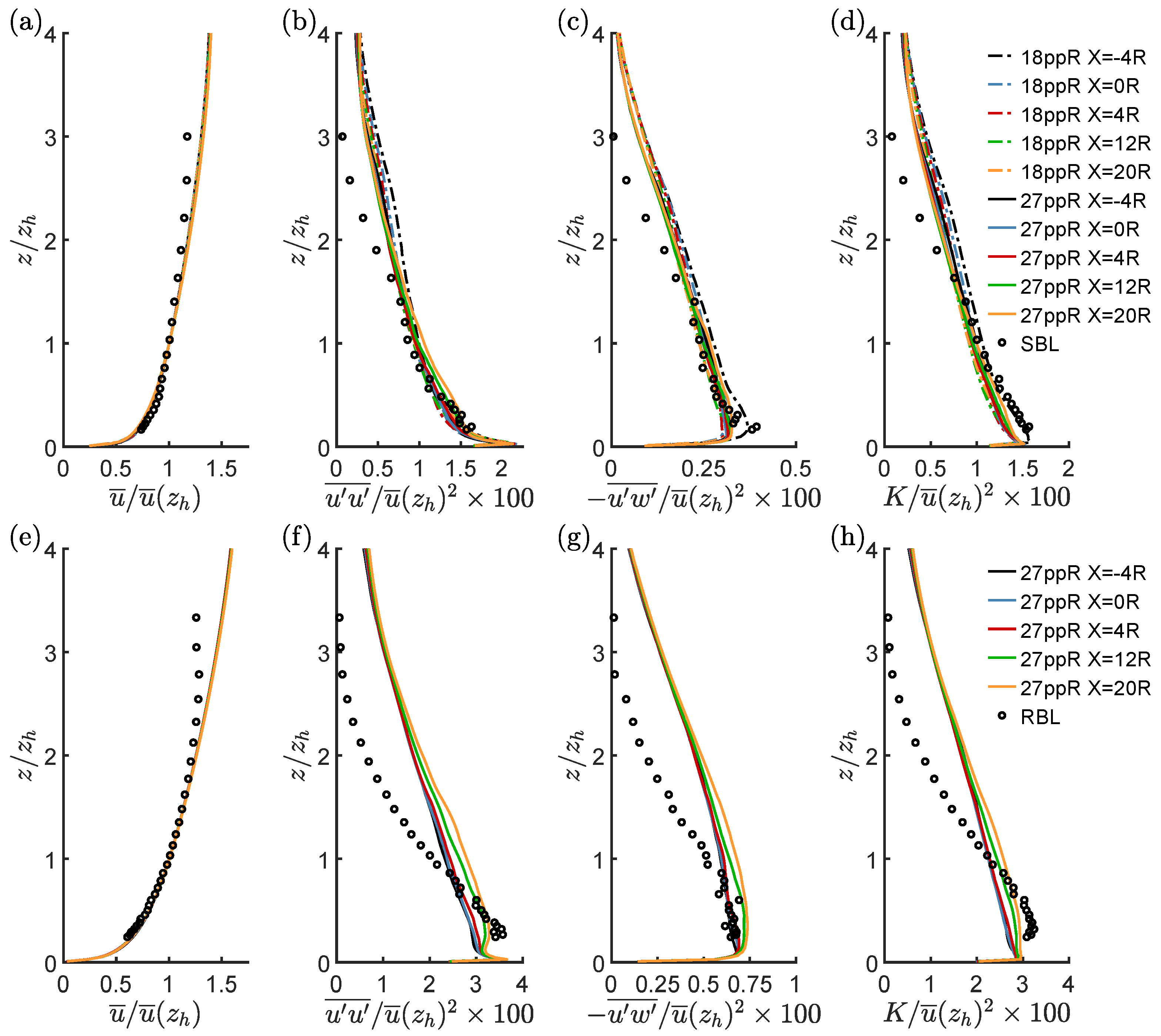
• For moderate roughness ($\alpha =0.16$), shear exponent, turbulence intensities and spectral densities of the approach flow match well with measurements in the lower half of the boundary layer.
• For high roughness ($\alpha =0.32$), a novel wall-model (virtually lifted wall) [14] was used: in this case, the match with the measured inflow is good at hub height, although not over the entire boundary layer.
• Erroneous values of turbulence intensities in wall-adjacent cell layers resulting from short-comings of the wall-stress model do not adversely affect the wake evolution.
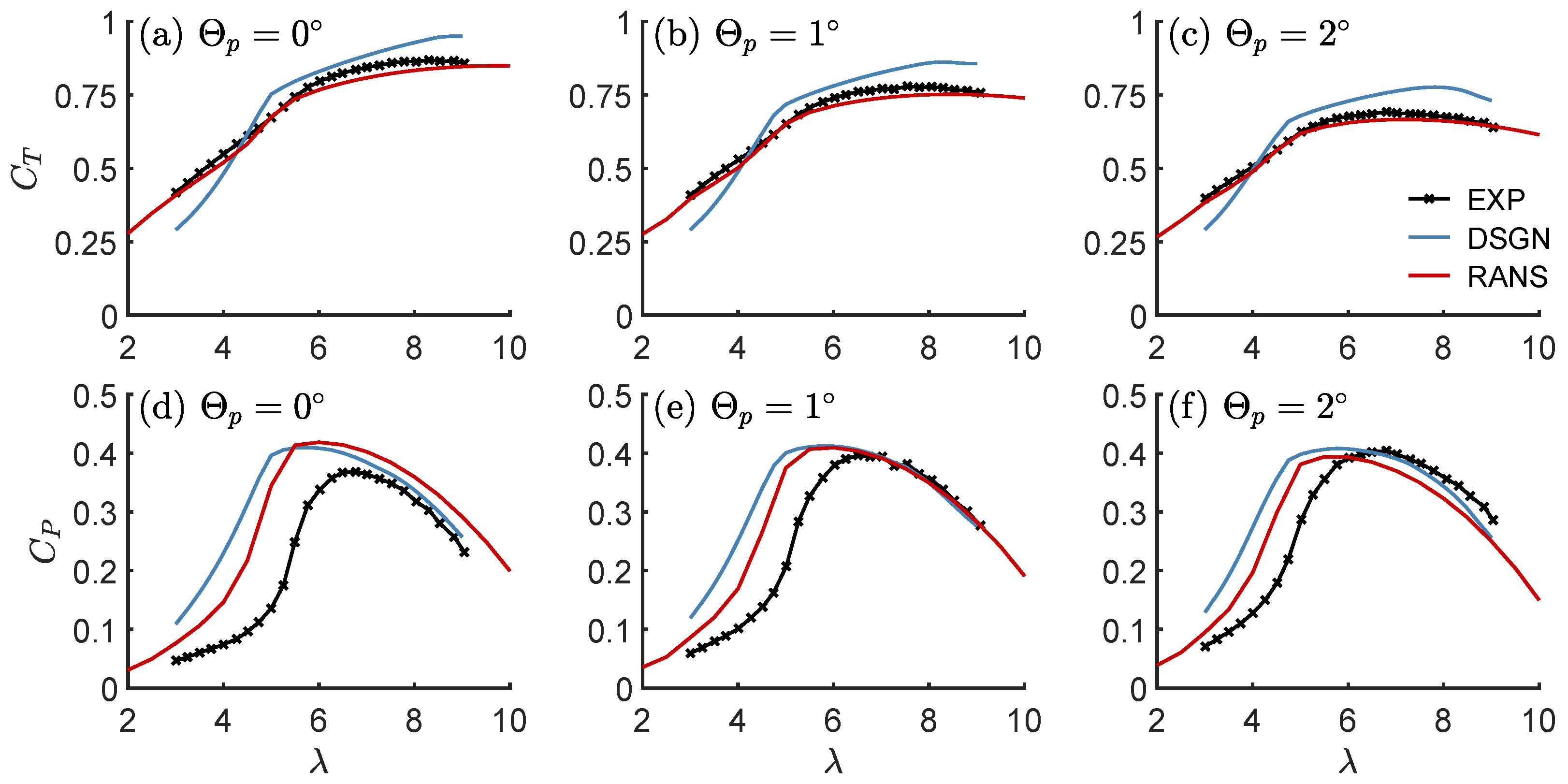
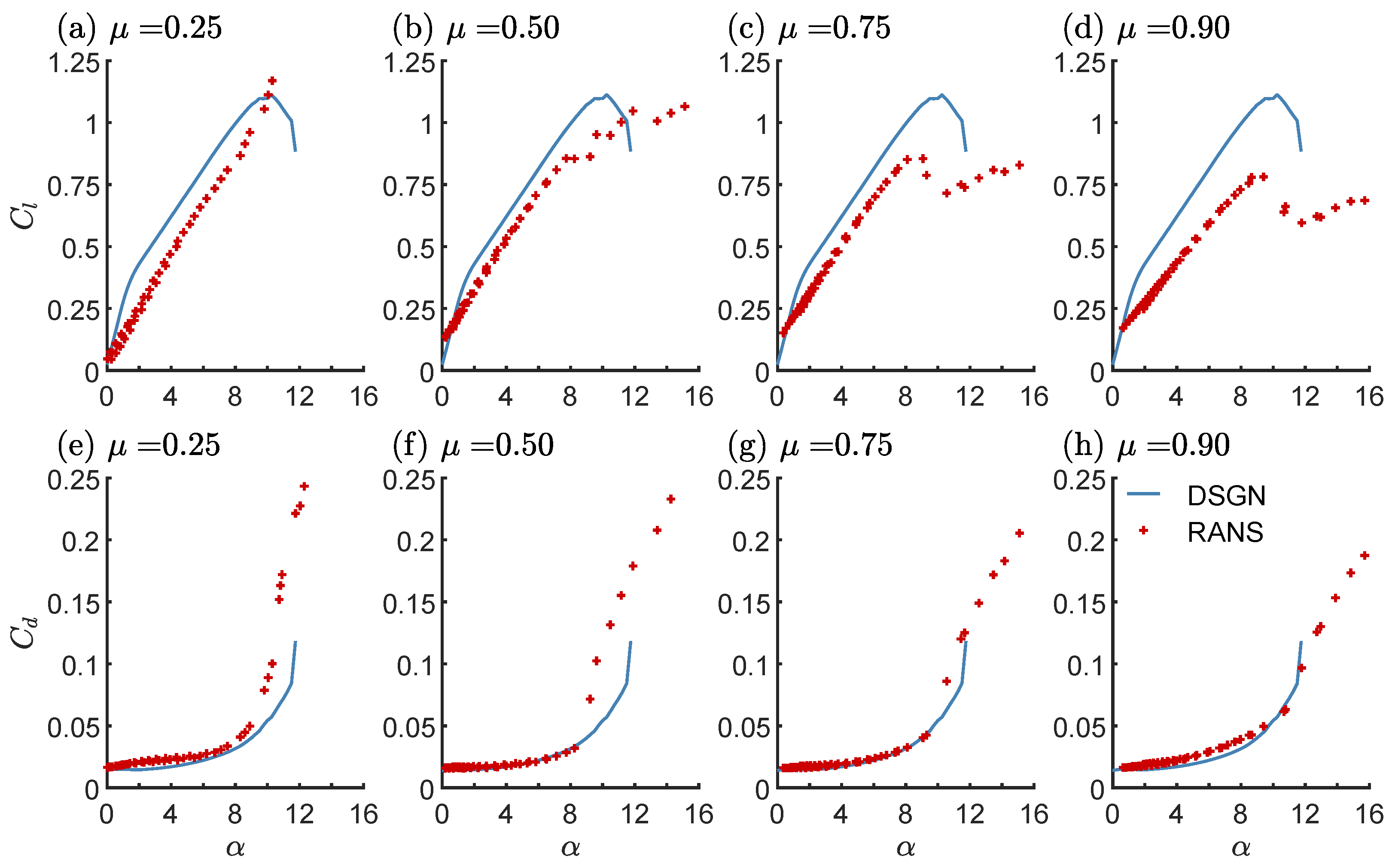
• Actuator line (ALM) rotor modeling works best if the blade polar identification is based on an inverted blade element momentum theory in conjunction with 3D-RANS simulation of the blade geometry of the wind turbine model.
• In the near wake ($x=2R$), the mean flow matches well, whereas turbulence intensities in the LES do not reach the same maxima associated with the formation and break-down of tip vortices as the experimental data, probably due to limitations of the ALM method.
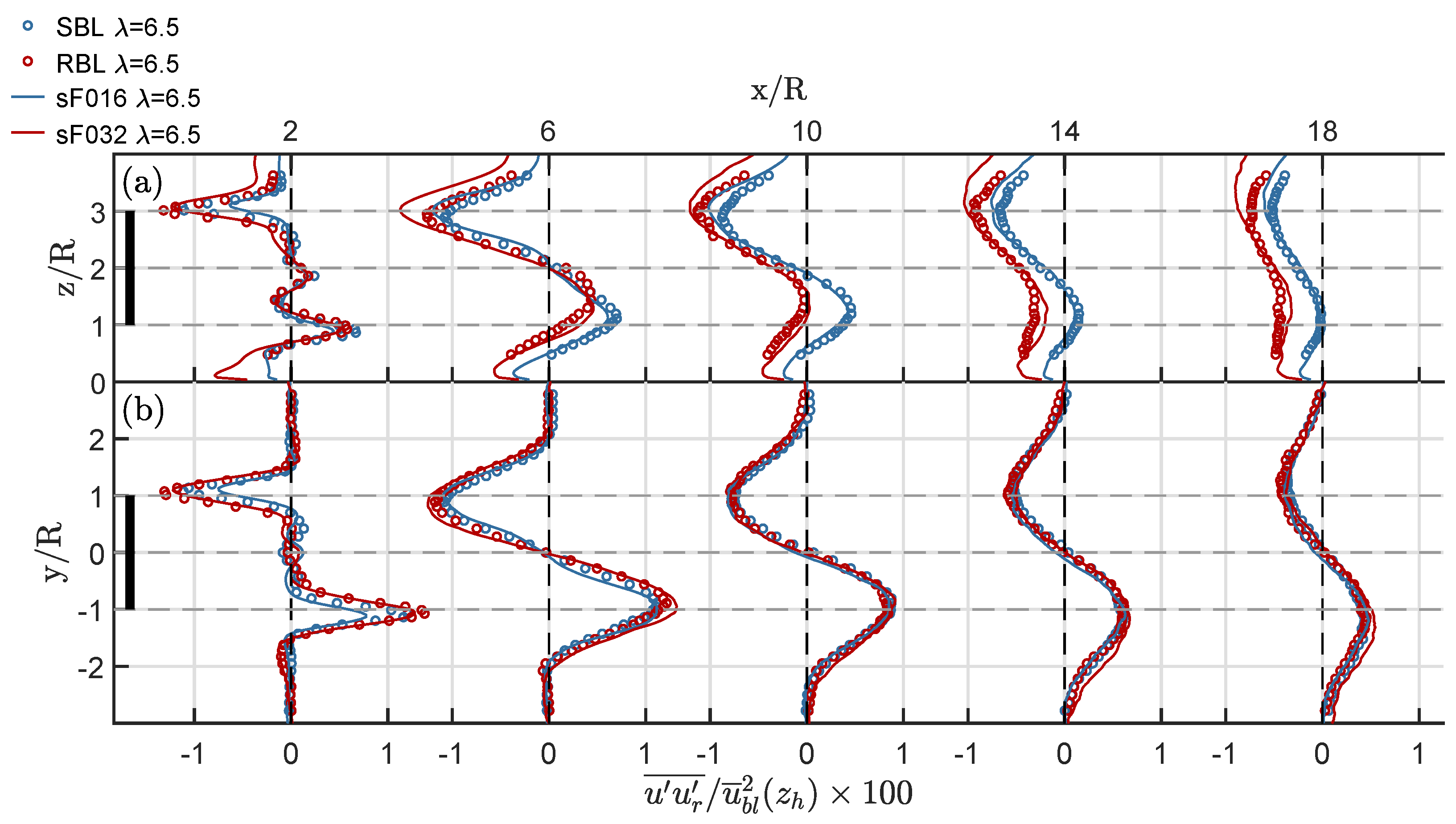
• In the far wake, $x>6R$, lateral profiles of mean flow, Reynolds shear stresses and turbulence intensities in a wall-parallel plane at hub height match better with measurements then profiles in a vertical plane through the wake center.
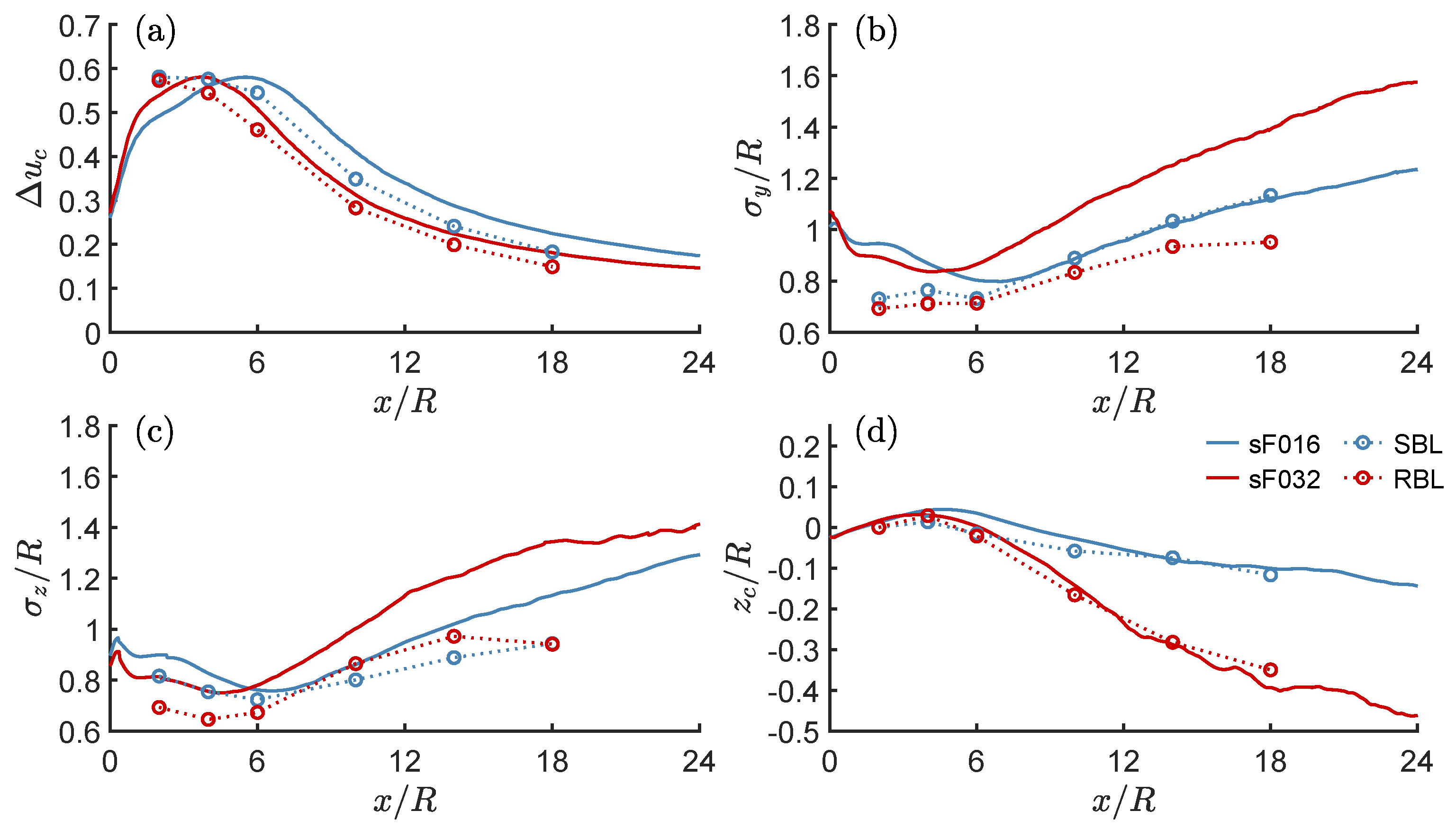
• An axial shift in the wake deficit $\Delta u$ is associated with overprediction of the wake depth. Nevertheless, the change rates $d\Delta u/dx$ are well reproduced. Whereas the influence of roughness on the vertical wake deflection is well captured, its impact on the wake width is larger in the LES than in the reference experiment.
• The remaining differences between simulation and measurements can not be tracked down to a single cause; they can be interpreted as a limit for the achievable accuracy with the current approach.

Overall, the numerical simulation captures quantitatively very well the relative changes in profiles of mean axial flow, shear stresses and turbulence intensities associated with the change in ground roughness. The same holds for the wake deficit, the vertical wake deflection and the change rates of the vertical wake width. Thus, the generated simulation data base can be explored in more detail in order to identify physical processes from the analysis of the relevance of individual terms in the balance equations for momentum and turbulence kinetic energy. This might be helpful in the development and improvement of fast wake prediction models that take roughness into account, as proposed in [15]. As a first step towards this goal, the LES database was used by Stein [14] to identify remarkable changes in the structure of the lateral momentum budget under the combined influence of roughness and yaw misalignment.

References

1. Knudsen, T.; Bak, T.; Svenstrup, M. Survey of wind farm control—Power and fatigue optimization. Wind Energy 2015, 18, 1333–1351. [Google Scholar] [CrossRef]
2. Abkar, M.; Porté-Agel, F. Influence of atmospheric stability on wind-turbine wakes: A large-eddy simulation study. Phys. Fluids 2015, 27, 035104. [Google Scholar] [CrossRef] [Green Version]
3. Vollmer, L.; Steinfeld, G. Estimating the wake deflection downstream of a wind turbine in different atmospheric stabilities: An LES study. Wind Energ. Sci. 2016, 1, 129–141. [Google Scholar] [CrossRef] [Green Version]
4. Hsieh, A.S.; Brown, K.A.; deVelder, N.B.; Herges, T.G.; Knaus, R.C. High-fidelity wind farm simulation methodology with experimental validation. J. Wind. Eng. Ind. Aerodyn. 2021, 218, 104754. [Google Scholar] [CrossRef]
5. Vermeer, L.; Sørensen, J.; Crespo, A. Wind turbine wake aerodynamics. Prog. Aerosp. Sci. 2003, 39, 467–510. [Google Scholar] [CrossRef]
6. Porté-Agel, F.; Bastankhah, M.; Shamsoddin, S. Wind-Turbine and Wind-Farm Flows: A Review. Bound.-Layer Meteorol. 2020, 174, 1–59. [Google Scholar] [CrossRef] [Green Version]
7. Sørensen, J.; Mikkelsen, R.F.; Henningson, D.S.; Ivanell, S.; Sarmast, S.; Andersen, S.J. Simulation of wind turbine wakes using the actuator line technique. Philos. Trans. R. Soc. A Math. Phys. Eng. Sci. 2015, 373, 20140071. [Google Scholar] [CrossRef] [Green Version]
8. Barlas, E.; Buckingham, S.; van Beeck, J. Roughness Effects on Wind-Turbine Wake Dynamics in a Boundary-Layer Wind Tunnel. Bound.-Layer Meteorol. 2016, 158, 27–42. [Google Scholar] [CrossRef] [Green Version]
9. Zhang, W.; Markfort, C.; Porté-Agel, F. Near-wake flow structure downwind of a wind turbine in a turbulent boundary layer. Exp. Fluids 2011, 52, 1219–1235. [Google Scholar] [CrossRef] [Green Version]
10. Chamorro, L.; Porté-Agel, F. A Wind-Tunnel Investigation of Wind-Turbine Wakes: Boundary-Layer Turbulence Effects. Bound.-Layer Meteorol. 2009, 132, 129–149. [Google Scholar] [CrossRef] [Green Version]
11. Wu, Y.; Porté-Agel, F. Atmospheric Turbulence Effects on Wind-Turbine Wakes: An LES Study. Energies 2012, 5, 5340–5362. [Google Scholar] [CrossRef]
12. Jin, Y. Effects of Freestream Turbulence in a Model Wind Turbine Wake. Energies 2016, 9, 830. [Google Scholar] [CrossRef] [Green Version]
13. ESDU. Engineering Sciences Data Unit. Characteristics of Atmospheric Turbulence Near the Ground; Part II: Single Point Data for Strong Winds (Neutral Atmosphere); ESDU International, Item No. 85020; ESDU: London, UK, 2001; ISBN 978-0-85679-526-7. [Google Scholar]
14. Stein, V. Analysis of Wind Turbine Wakes Immersed in Turbulent Boundary Layer Flows over Rough Surfaces-An Experimental and Numerical Study. Ph.D. Thesis, Technical University Munich, München, Germany, 2022. [Google Scholar]
15. Stein, V.; Kaltenbach, H.J. Non-Equilibrium Scaling Applied to the Wake Evolution of a Model Scale Wind Turbine. Energies 2019, 12, 2763. [Google Scholar] [CrossRef] [Green Version]
16. Counihan, J. An improved method of simulating an atmospheric boundary layer in a wind tunnel. Atmos. Environ. 1969, 3, 197–214. [Google Scholar] [CrossRef]
17. Sørensen, J.; Myken, A. Unsteady actuator disc model for horizontal axis wind turbines. J. Wind. Eng. Ind. Aerodyn. 1992, 39, 139–149. [Google Scholar] [CrossRef]
18. Jiménez, A.; Crespo, A.; Migoya, E.; Garcia, J. Advances in large-eddy simulation of a wind turbine wake. J. of Phys. Conf. Ser. 2007, 75, 01204. [Google Scholar] [CrossRef]
19. Jiménez, A.; Crespo, A.; Migoya, E.; Garcia, J. Large-eddy simulation of spectral coherence in a wind turbine wake. Environ. Res. Lett. 2008, 3, 015004. [Google Scholar] [CrossRef]
20. Sørensen, J.; Shen, W. Numerical modelling of Wind Turbine Wakes. J. Fluids Eng. 2002, 124, 393–399. [Google Scholar] [CrossRef]
21. Mikkelsen, R. Actuator Disc Methods Applied to Wind Turbines. Ph.D. Thesis, Technical University of Denmark, Roskilde, Denmark, 2003. [Google Scholar]
22. Wu, Y.; Porté-Agel, F. Large-eddy simulation of wind-turbine wakes: Evaluation of turbine parametrisations. Bound.-Layer Meteorol. 2011, 138, 345–366. [Google Scholar] [CrossRef]
23. Jiménez, J. Turbulent Flows over Rough Walls. Annu. Rev. Fluid Mech. 2004, 36, 173–196. [Google Scholar] [CrossRef]
24. Castro, I. Rough-wall boundary layers: Mean flow universality. J. Fluid Mech. 2007, 585, 469–485. [Google Scholar] [CrossRef] [Green Version]
25. Schumann, U. Subgrid Scale Model for Finite Difference Simulation of Turbulent Flows in Plane Channels and Annuli. J. Comput. Phys. 1975, 18, 376–404. [Google Scholar] [CrossRef] [Green Version]
26. Grötzbach, G. Direct numerical and large eddy simulation of turbulent channel flows. In Encyclopedia of Fluid Mechanics, Vol.6—Complex Flow Phenomena and Modeling; Gulf Publ. Co.: Houston, TX, USA, 1987. [Google Scholar]
27. Mason, P.; Thomson, D. Large-eddy simulations of the neutral-static-stability planetary boundary layer. Q. J. R. Meteorol. Soc. 1987, 113, 413–443. [Google Scholar] [CrossRef]
28. Mason, P.; Callen, N. On the magnitude of the subgrid-scale eddy coefficient in large-eddy simulations of turbulent channel flow. J. Fluid Mech. 1986, 162, 439–462. [Google Scholar] [CrossRef]
29. Larsson, J.; Kawai, S. Wall-Modeling in Large Eddy Simulation: Length Scales, Grid Resolution and Accuracy; Annual Research Briefs; Center for Turbulence Research: Stanford, CA, USA, 2010. [Google Scholar]
30. Leonard, A. Energy cascade in large eddy simulations of turbulent fluid flows. Adv. Geophys. 1974, 18A, 237–248. [Google Scholar]
31. Smagorinsky, J. General circulation experiments with the primitive equations, Part 1: The basic experiment. Mon. Weath. Rev. 1963, 91, 99–164. [Google Scholar] [CrossRef]
32. Germano, M.; Piomelli, U.; Moin, P.; Cabot, W. A dynamic subgrid-scale eddy viscosity model. Phys. Fluids A 1991, 3, 1760–1765. [Google Scholar] [CrossRef] [Green Version]
33. Tossas, L.A.M.; Leonardi, S. Wind Turbine Modeling for Computational Fluid Dynamics, December 2010–December 2012; Report NREL/SR-5000-55054; National Renewable Energy Lab. (NREL): Golden, CO, USA, 2013.
34. Porté-Agel, F.; Meneveau, C.; Parlange, M. A scale-dependent dynamic model for large-eddy simulation: Application to a neutral atmospheric boundary layer. J. Fluid Mech. 2000, 415, 261–284. [Google Scholar] [CrossRef] [Green Version]
35. Bou-Zeid, E.; Meneveau, C.; Parlange, M. A scale-dependent Lagrangian dynamic model for large-eddy simulation of complex turbulent flows. Phys. Fluids 2005, 17, 025105. [Google Scholar] [CrossRef] [Green Version]
36. Sarlak, H.; Meneveau, C.; Sørensen, J. Role of subgrid-scale modeling in large eddy simulation of wind turbine wake interactions. Renew. Energy 2015, 77, 386–399. [Google Scholar] [CrossRef]
37. Ghosal, S. An analysis of numerical errors in large-eddy simulations of turbulence. J. Comput. Phys. 1996, 125, 187–206. [Google Scholar] [CrossRef] [Green Version]
38. Hickel, S.; Adams, N.; Domaradzki, J. An adaptive local deconvolution method for implicit LES. J. Comput. Phys. 2006, 213, 413–436. [Google Scholar] [CrossRef]
39. Tabor, G.; Baba-Ahmadi, M. Inlet conditions for large eddy simulation: A review. Comput. Fluids 2010, 39, 553–567. [Google Scholar] [CrossRef]
40. Dhamankar, N.; Blaisdell, G. An Overview of Turbulent Inflow Boundary Conditions for Large Eddy Simulations. In Proceedings of the 22nd AIAA Computational Fluid Dynamics Conference AIAA 2015-3213, AIAA, Dallas, TX, USA, 22–26 June 2015. [Google Scholar]
41. Lund, T.; Wu, X.; Squires, K. Generation of turbulent inflow data for spatially-developing boundary layer simulations. J. Comp. Phys. 1998, 140, 233–258. [Google Scholar] [CrossRef] [Green Version]
42. Stevens, R.; Graham, J.; Meneveau, C. A concurrent precursor inflow method for Large Eddy Simulations and applications to finite length wind farms. Renew. Energy 2014, 68, 46–50. [Google Scholar] [CrossRef] [Green Version]
43. Mann, J. The spatial structure of neutral atmospheric surface-layer turbulence. J. Fluid Mech. 1994, 273, 141–168. [Google Scholar] [CrossRef]
44. Troldborg, N.; Sørensen, N.; Mikkelsen, R. Numerical Simulations of Wakes of Wind Turbines Operating in Sheared and Turbulent Inflow. In Proceedings of the European Wind Energy Conference, Marseille, France, 16–19 March 2009. [Google Scholar]
45. Troldborg, N.; Zahle, F.; Réthoré, P.; Sørensen, N. Comparison of wind turbine wake properties in non-sheared inflow predicted by different computational fluid dynamics rotor models. Energies 2014, 18, 1239–1250. [Google Scholar] [CrossRef]
46. Purohit, S.; Kabir, I.; Ng, E. On the accuracy of uRANS and LES-based CFD modeling approaches for rotor and wake aerodynamics of the (New) MEXICO wind turbine rotor phase-iii. Energies 2021, 14, 5198. [Google Scholar] [CrossRef]
47. Uchida, T.; Gagnon, Y. Effects of continuously changing inlet wind direction on near-to-far wake characteristics behind wind turbines over flat terrain. J. Wind. Eng. Ind. Aerodyn. 2022, 220, 104869. [Google Scholar] [CrossRef]
48. Xue, F.; Heping, D.; Xu, C.; Han, X.; Shangguan, Y.; Li, T.; Fen, Z. Research on the Power Capture and Wake Characteristics of a Wind Turbine Based on a Modified Actuator Line Model. Energies 2022, 15, 282. [Google Scholar] [CrossRef]
49. Draper, M.; Guggeri, A.; Mendina, M.; Usera, G.; Campagnolo, F. A large eddy simulation-actuator line model framework to simulate a scaled wind energy facility and its application. J. Wind Eng. Ind. Aerodyn. 2018, 182, 146–159. [Google Scholar] [CrossRef]
50. Stevens, R.J.; Martínez-Tossas, L.A.; Meneveau, C. Comparison of wind farm large eddy simulations using actuator disk and actuator line models with wind tunnel experiments. Renew. Energy 2018, 116, 470–478. [Google Scholar] [CrossRef]
51. Wang, J.; Wang, C.; Campagnolo, F.; Bottasso, C.L. Wake behavior and control: Comparison of LES simulations and wind tunnel measurements. Wind Energ. Sci. 2019, 4, 71–88. [Google Scholar] [CrossRef] [Green Version]
52. Wang, C.; Campagnolo, F.; Canet, H.; Barreiro, D.; Bottasso, C.L. How realistic are the wakes of scaled wind turbine models? Wind Energ. Sci. 2021, 6, 961–981. [Google Scholar] [CrossRef]
53. Stein, V.; Kaltenbach, H.J. Influence of ground roughness on the wake of a yawed wind turbine—A comparison of wind-tunnel measurements and model predictions. J. Phys. Conf. Ser. 2018, 1037, 072005. [Google Scholar] [CrossRef]
54. Hickel, S.; Adams, N. Efficient Implementation of Nonlinea Deconvolution Methods for Implicit Large-Eddy Simulation. In High Performance Computing in Science and Engineering’06; Springer: Berlin/Heidelberg, Germany, 2007. [Google Scholar]
55. Remmler, S.; Hickel, S. Direct and large eddy simulation of stratified turbulence. J. Heat Fluid Flow 2012, 35, 13–24. [Google Scholar] [CrossRef]
56. Hickel, S.; Adams, N. On implicit subgrid-scale modeling in wall-bounded flows. Phys. Fluids 2007, 19, 105106. [Google Scholar] [CrossRef]
57. Hickel, S.; Adams, N.; Mansour, N.N. Implicit subgrid-scale modeling for large-eddy simulation of passive-scalar mixing. Phys. Fluids 2007, 19, 095102. [Google Scholar] [CrossRef] [Green Version]
58. Zwerger, C.; Hickel, S.; Breitsamter, C.; Adams, N. Wall modeled large-eddy simulation of the VFE-2 delta wing. In Direct and Large-Eddy Simulation X; Springer: Berlin/Heidelberg, Germany, 2015. [Google Scholar]
59. Cabot, W.; Moin, P. Approximate wall boundary conditions in the large-eddy simulation of high Reynolds number flow. Flow Turbul. Combust. 1999, 63, 269–291. [Google Scholar] [CrossRef]
60. Nicoud, F.; Baggett, J.; Moin, P.; Cabot, W. Large eddy simulation wall-modeling based on suboptimal control theory and linear stochastic estimation. Phys. Fluids 2001, 13, 2968–2984. [Google Scholar] [CrossRef]
61. Heist, D.K.; Castro, I. Combined laser-doppler and cold wire anemometry for turbulent heat flux measurement. Exp. Fluids 1998, 24, 375–381. [Google Scholar] [CrossRef]
62. Piomelli, U. Wall-layer models for large-eddy simulations. Prog. Aerosp. Sci. 2008, 44, 437–446. [Google Scholar] [CrossRef]
63. Davidson, L. Large Eddy Simulations: How to evaluate resolution. Int. J. Heat Fluid Flow 2009, 30, 1016–1025. [Google Scholar] [CrossRef] [Green Version]
64. Piomelli, U.; Balaras, E.; Pasinato, H.; Squires, K.; Spalart, P.R. The inner–outer layer interface in large-eddy simulations with wall-layer models. Int. J. Heat Fluid Flow 2003, 24, 538–550. [Google Scholar] [CrossRef] [Green Version]
65. Saito, N.; Pullin, D.; Inoue, M. Large eddy simulation of smooth-wall, transitional and fully rough-wall channel flow. Phys. Fluids 2012, 24, 075103. [Google Scholar] [CrossRef] [Green Version]
66. Flores, O.; Jiménez, J. Effect of wall-boundary disturbances on turbulent channel flows. J. Fluid Mech. 2006, 566, 357–376. [Google Scholar] [CrossRef]
67. Schneider, M.; Nitzsche, J.; Hennings, H. Accurate load prediction by BEM with airfoil data from 3D RANS simulations. J. Phys. Conf. Ser. 2016, 753, 082016. [Google Scholar] [CrossRef] [Green Version]
68. Wimshurst, A.; Willden, R. Extracting lift and drag polars from blade- resolved computational fluid dynamics for use in actuator line modelling of horizontal axis turbines. Wind Energy 2017, 20, 815–833. [Google Scholar] [CrossRef]
69. Hansen, M. Aerodynamics of Windturbines, 3rd ed.; Earthscan from Routledge: London, UK, 2015. [Google Scholar]
70. Burton, T.; Jenkins, N.; Sharpe, D.; Bossanyi, E. Wind Energy Handbook; John Wiley & Sons: Chichester, UK, 2011; ISBN 978-0-470-69975-1. [Google Scholar]
71. Chamorro, L.P.; Arndt, R.E.; Sotiropoulos, F. Reynolds number dependence of turbulence statistics in the wake of wind turbines. Wind Energ. 2012, 15, 733–742. [Google Scholar] [CrossRef]
Figure 1. Non-dimensional mean axial velocity u + as function of normalized wall distance z / δ computed using the m-th grid point off the wall, indicated by colored dots as denoted in the legend. The black dashed straight line marks the logarithmic law for a rough wall with δ / z 0 = 4500 .
Energies 15 02579 g001
Figure 2. Reynolds stresses normalized by u τ 2 : (a) u u ¯ + , (b) w w ¯ + , (c) v v ¯ + and (d) u w ¯ + as function of normalized wall distance z / δ for different off-wall position z m .
Energies 15 02579 g002
Figure 3. Non-dimensional Reynolds stresses (a) u u ¯ + , (b) w w ¯ + , (c) v v ¯ + and (d) u w ¯ + as function of normalized wall distance z / δ for three different grid resolutions indicated in the legend.
Energies 15 02579 g003
Figure 4. Comparison of (ac) thrust C T and (df) power coefficient C P as a function of tip speed ratio λ obtained from measurement (EXP), 2D airfoil calculations (DSGN) and numerical simulation (RANS) for pitch angles Θ p = 0 , 1 , 2 .
Energies 15 02579 g004
Figure 5. Comparison of blade polars obtained from 2D airfoil calculations (DSGN), and numerical simulation (RANS): (ad) lift C l and (eh) drag C d coefficients as function of AoA θ at selected blade sections μ = r / R = 0.25 , 0.5 , 0.75 , 0.9 .
Energies 15 02579 g005
Figure 6. Sketch of the computational domain used in the LES of the model wind turbine.
Energies 15 02579 g006
Figure 7. (a) Mean axial velocity u ¯ ( x , z h ) and (b) turbulent kinetic energy K ( x , z h ) as function of the axial distance to the rotor, both normalized to their respective values u ¯ ( x r , z h ) , K ( x r , z h ) at the rotor center along the entire domain without turbine. The dashed vertical lines indicate the borders between the regions and the legend denotes flow condition and grid resolution.
Energies 15 02579 g007
Figure 8. Vertical profiles at selected locations in the wake region of the empty domain for intermediate roughness ( α = 0.16 , top row) and large roughness ( α = 0.32 , bottom row): (a,e) mean axial velocity u ¯ ; (b,f) axial intensity u u ¯ ; (c,g) Reynolds shear stress u w ¯ ; (d,h) turbulent kinetic energy K; all normalized with the reference speed u ¯ h = u ¯ ( x r , z h ) .
Energies 15 02579 g008
Figure 9. Normalized energy spectral density of the three velocity components at the rotor center S u i u j ( z h ) / u i u j ¯ ( z h ) with i = j , within simulated boundary layers and experimental SBL configuration: (a,d) u -component; (b,e) v -component and (c,f) w -component. The legend denotes flow conditions, dashed lines denote the slope of the Kolmogorov cascade.
Energies 15 02579 g009
Figure 10. Comparison of measurements and numerical results for (a) power C P and (b) thrust coefficient C T as function of yaw angle γ . The legend states the flow conditions.
Energies 15 02579 g010
Figure 11. Profiles of the normalized mean axial velocity component u ¯ / u ¯ b l ( z h ) in the (a) mid-vertical and (b) mid-horizontal plane at axial positions x / R = 2, 6, 10, 14, 18. Symbols denote measurements, whereas lines correspond to LES results. The legend denotes the case. The origin of local coordinates in the upper subfigure is located at x = 0.8 and in the lower subfigure at x = 1 .
Energies 15 02579 g011
Figure 12. Profiles of the normalized Reynolds shear stress (a) u w ¯ / u ¯ h 2 in the mid-vertical and (b) u v ¯ / u ¯ h 2 the mid-horizontal plane at axial positions x / R = 2, 6, 10, 14, 18. Symbols denote measurements, whereas lines correspond to LES results. The legend denotes the case.
Energies 15 02579 g012
Figure 13. Profiles of the turbulence intensities in axial direction u u ¯ (top), in lateral direction v v ¯ and in vertical (wall-normal) direction w w ¯ (bottom), normalized by u ¯ h 2 in (a,c,e) mid-vertical and (b,d,f) mid-horizontal planes at axial positions x / R = 2, 6, 10, 14, 18. Circles denote measurements, whereas lines correspond to LES results. The color code denotes the shear exponent α = 0.16 (blue) and α = 0.32 (red).
Energies 15 02579 g013
Figure 14. Profiles of the normalized turbulent kinetic energy K / u ¯ h 2 in the (a) mid-vertical and (b) mid-horizontal plane at axial positions x / R = 2, 6, 10, 14, 18. Symbols denote measurements, whereas lines correspond to LES results. The legend denotes the case.
Energies 15 02579 g014
Figure 15. Wake parameters of the model wind turbine operating at design tip-speed ratio above moderate (SBL) and high (RBL) ground roughness: (a) centerline velocity deficit Δ u C , (b) lateral σ y and (c) vertical half width σ z , and (d) vertical centerline position z C . The legend indicates the flow condition.
Energies 15 02579 g015