Application of Machine Learning to Predict the Performance of an EMIPG Reactor Using Data from Numerical Simulations

Abstract

Microwave-driven plasma gasification technology has the potential to produce clean energy from municipal and industrial solid wastes. It can generate temperatures above 2000 K (as high as 30,000 K) in a reactor, leading to complete combustion and reduction of toxic byproducts. Characterizing complex processes inside such a system is however challenging. In previous studies, simulations using computational fluid dynamics (CFD) produced reproducible results, but the simulations are tedious and involve assumptions. In this study, we propose machine-learning models that can be used in tandem with CFD, to accelerate high-fidelity fluid simulation, improve turbulence modeling, and enhance reduced-order models. A two-dimensional microwave-driven plasma gasification reactor was developed in ANSYS (Ansys, Canonsburg, PA, USA) Fluent (a CFD tool), to create 644 (geometry and temperature) datasets for training six machine-learning (ML) models. When fed with just geometry datasets, these ML models were able to predict the proportion of the reactor area with temperature above 2000 K. This temperature level is considered a benchmark to prevent formation of undesirable byproducts. The ML model that achieved highest prediction accuracy was the feed forward neural network; the mean absolute error was 0.011. This novel machine-learning model can enable future optimization of experimental microwave plasma gasification systems for application in waste-to-energy.

1. Introduction

The global human population is expected to increase from 7.8 billion to 10.9 billion throughout the course of the 21st century [1]. The growth in the global population results in the greater consumption of resources and consequently drives an increasing municipal solid waste (MSW) stream [2]. Furthermore, rapid urbanization and economic development accompany this global population rise and concentrate MSW into confined, metropolitan areas [2,3,4]. Increased production and concentration of MSW in tandem with a rising composition complexity poses a glaring challenge for proper waste management [5]. Of the globally estimated 2.01 billion tons of MSW currently generated annually, approximately 33% is not managed properly [6].

Proper management of MSW is essential for preserving the welfare of society. MSW has the ability to affect air, water, and soil vectors that directly impact human health [7], [8]. The two predominant global means of managing MSW today are landfilling and incineration [6]. Unfortunately, both means of management and disposal can lead to inadvertent negative effects even when conducting proper management procedures. Landfills are some of the most significant contributors to greenhouse gas emissions within the waste industry and, in developing countries, landfill methane is rising in conjunction with population, consumption, and landfill expansion [2,8,9]. Waste incineration can cause a detriment to public health and the environment by creating sulfur oxides, nitrogen oxides, and particulate matter from the combustion process [10,11]. Additionally, the increasing complexity of the composition of MSW causes incineration to yield a wide range of toxic and carcinogenic contaminants such as polyvinyl chloride, heavy metals, organic chemicals, and polychlorinated dibenzodioxins (dioxins) and polychlorinated dibenzofurans (furans) [2,12,13,14,15,16].

While known to be a global issue, smaller systems and environments also experience this waste management dilemma. The United States Department of Defense (USDOD) has recognized the need for process improvement within all of its operating centers [17,18,19,20]. Some factors driving the USDOD to pursue process improvement within waste management include: concerns about burn pit exposure causing adverse human health effects, limited energy resources and land availability in contingency operation environments, desire for point-of-source waste-to-energy (WtE) technologies, security concerns, and an overall transition towards more sustainable operations [21,22,23,24,25]. The National Aeronautics and Space Administration (NASA), in addition to other private and government space agencies, are concentrated on improving waste management processes. NASA and other space agencies desire this process improvement to ensure efficient use of resources in interplanetary space travel, and future colonization of terrestrial bodies, planets, and space stations [26]. Facilities such as hospitals and airports also must focus efforts on improving their waste management practices. During the peak period, the COVID-19 pandemic created an estimated five-fold increase in the demand for daily medical waste disposal, which threatened the resilience of medical emergency systems in urban areas [27]. Many airports generate waste volumes at the same rate as a small city, and regional and national governments in their jurisdiction emphasize waste diversion from landfills [28]. This focus on waste diversion for numerous airports leads to their pursuit of sustainable waste management practices [28].

One emerging technology that may help to solve the multivariate waste management problem is microwave induced plasma gasification (MIPG). MIPG is a WtE technology that utilizes plasma gasification as a thermal waste treatment process. Plasma gasification is a process that subjects the MSW to a plasma flame within a reactor where temperatures can exceed 10,000 K [29]. Once exposed to the extreme temperatures within the reactor, the MSW is converted into two products: a syngas primarily composed of carbon monoxide and hydrogen, and an inert slag [30]. Both products can be utilized as resources, promoting a sustainable waste management model. The syngas output can be utilized for energy production, and the inert slag can be used as a construction material [31,32]. The high temperature combustion is an enormous benefit for plasma gasification over other thermal waste treatment processes; this extreme temperature allows for hazardous and complex materials to be safely combusted without toxic emissions, dioxins, furans, or greenhouse gases [33,34]. Most MIPG systems initialize the plasma flame by inserting a tungsten rod that acts as a temporary electrode arrangement [35,36]. Once the plasma flame is initiated, the tungsten rod is removed and the plasma flame is maintained by a microwave and plasma-forming gases, rather than an electrode arrangement. This increases system resilience as electrode utilization and corrosion can cause multiple operational problems and efficiency losses in traditional plasma gasification systems [30], [37]. Additionally, MIPG systems maintain lower voltage requirements than other plasma generator methods and have a lower setup cost as the reactor can operate under atmospheric conditions [30,38]. 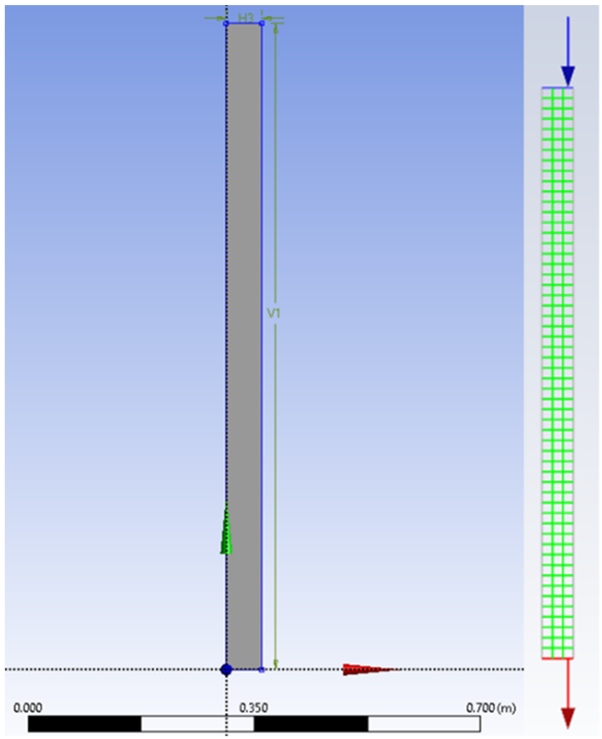One disadvantage of MIPG systems is that they are harder to scale than electrode-based systems [39]. Although MIPG systems can control the diameter and temperature of the plasma flame by increasing power to the system, the length of the reactor can only be controlled by adjusting the reactor size [40]. The diameter of the plasma flame is also constrained to the physical boundary of the reactor [40].

ANSYS Fluent is a software package that can be used to numerically model an MIPG system. Fluent is one of the most widely used computational fluid dynamics (CFD) modeling software packages in the world [41]. CFD is a tool originally used for aerospace applications; however, it has been adopted heavily in both the environmental and chemical engineering fields for its rich reactor modeling and solver ability [41,42,43,44]. CFD modeling software uses a chosen solver method to solve partial differential equations for mass, momentum, and energy, and their theoretical and empirical correlations [45]. When these models are synthesized, the physical–chemical phenomena that take place within an MIPG reactor can be simulated and observed [46,47]. By allowing the user to understand the multiphysics taking place within a MIPG reactor, expensive and tedious experimentation can be reduced and further optimized [45]. ANSYS Fluent offers some benefits over other CFD modeling software, especially for first time users. ANSYS Fluent contains an intuitive and robust graphical user interface (GUI) and a highly integrated support system [41]. Both the GUI and the support system aid the user to easily define solver settings for a model. A disadvantage of ANSYS Fluent is that it is a closed source platform, which can make it harder to modify the solver with user-defined functions (UDF) [48,49,50]. For simulations that necessitate a high degree of personalization and where the user has a firm grasp of how to modify and customize open-source software, OpenFOAM is a great alternative CFD modeling software package [41,51,52]. Machine-learning (ML) algorithms can be informed by numerical models in order to build an accurate representation of the modeled system [53]. Additionally, the synthesis of ML and numerical models has the potential to accelerate high-fidelity fluid simulation, improve turbulence modeling, and enhance reduced-order models [54]. ML algorithms identify patterns within a dataset. These algorithms have been shown to be very functional and accurate with non-linear and highly variable time-dependent data commonly found in plasma gasification reactors [55,56].

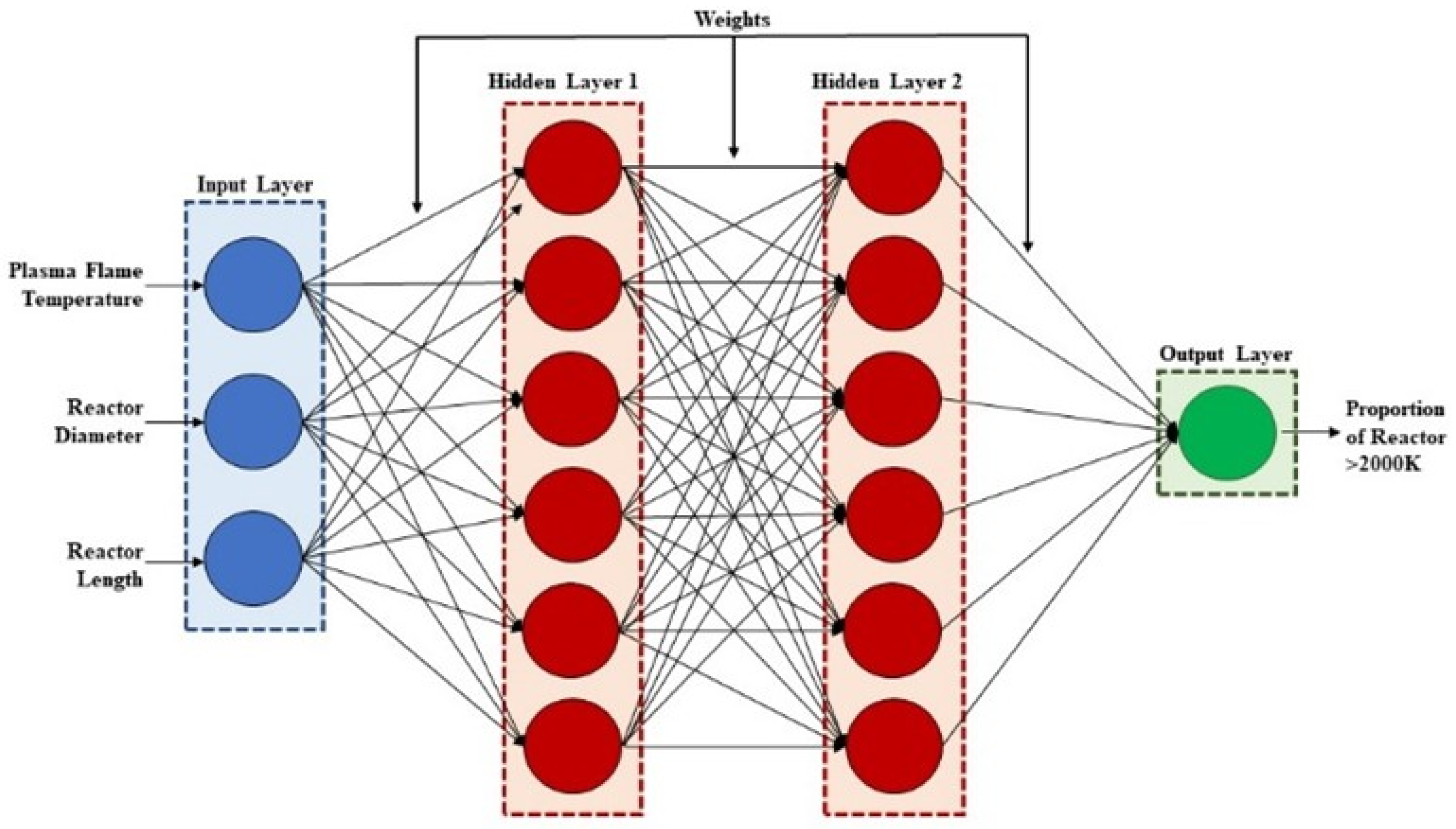
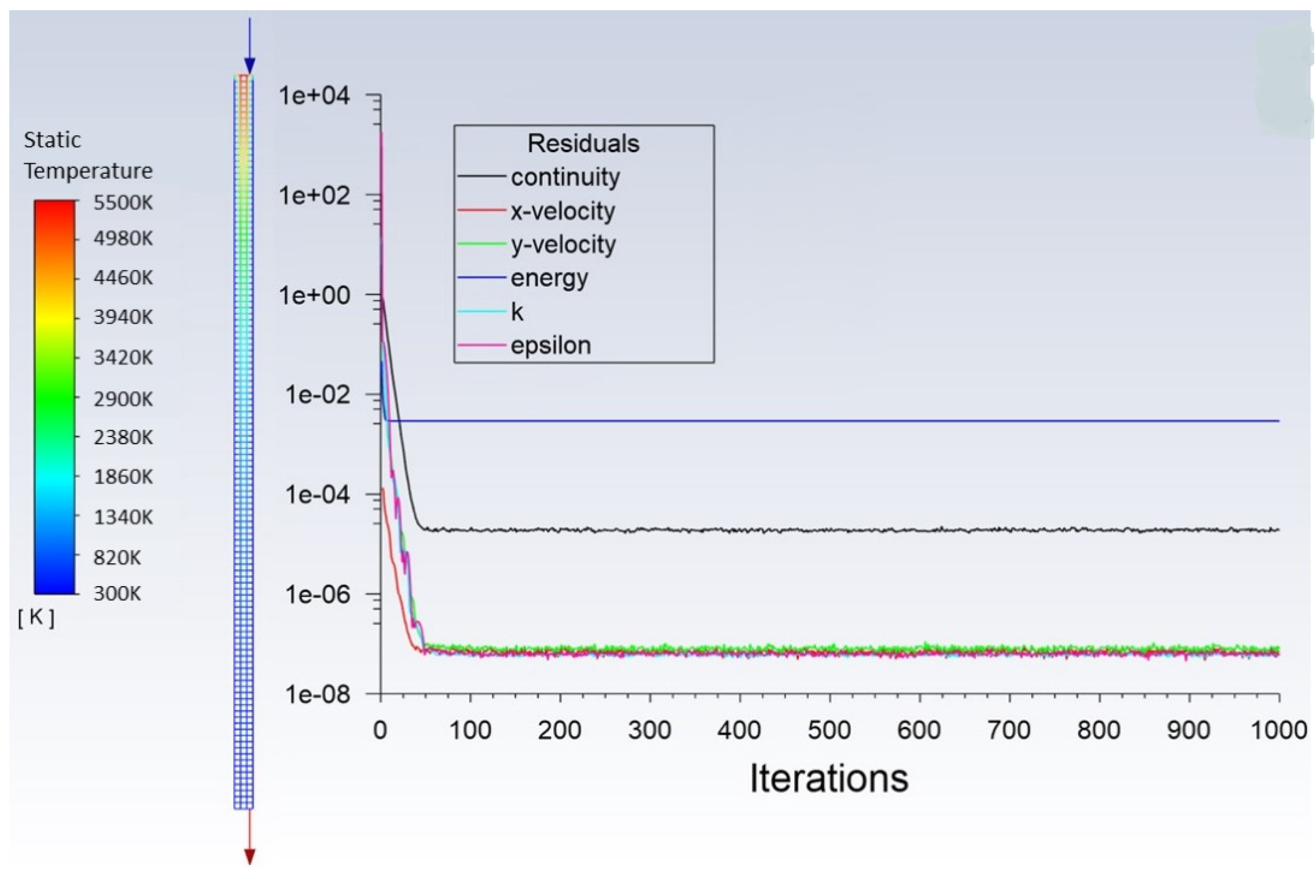
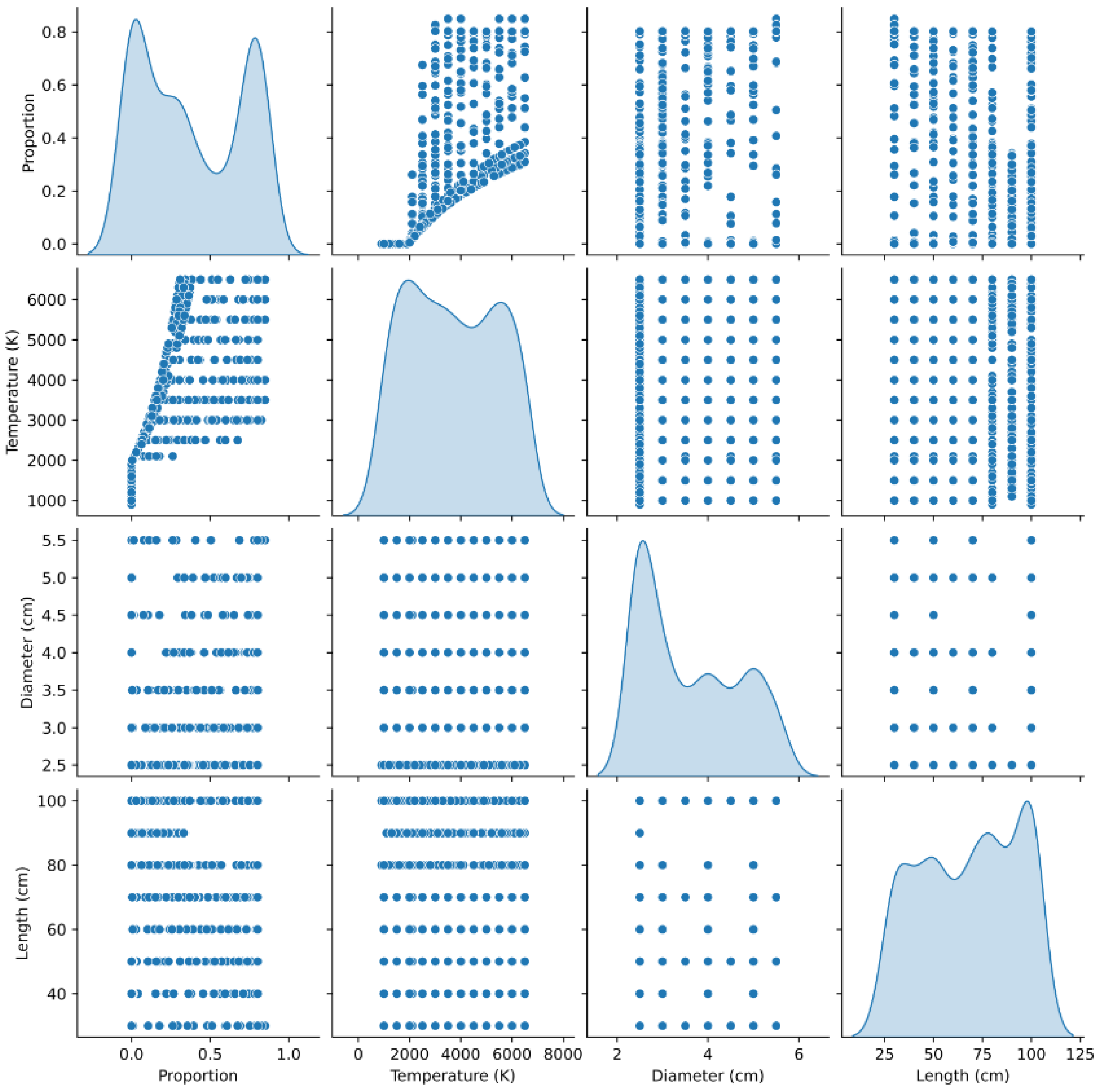
The purpose of this study was to compare ML algorithms that can predict the proportion of the area in the reactor that is above 2000 K within a two-dimensional (2D) MIPG reactor given geometry and temperature inputs. A total of 644 CFD models were simulated within ANSYS Fluent to create a dataset for the machine-learning algorithms. The geometry and temperature inputs within the CFD models were based on experimental MIPG (EMIPG) reactors from a literature review of 13 different experiments. Thermal plasma is commonly defined as the temperature range from approximately 2000 to 30,000 K and, by staying in this temperature range, full combustion of the waste can be achieved [57]. A magnetron is responsible for providing the microwave to the reactor, and the power supply to it has a direct effect on the temperature of the plasma flame within the EMIPG [58]. G.S. Ho et al. determined that fuel retention time, the amount of time that the MSW has in contact with the plasma flame, is the key parameter that affects plasma gasification performance [38]. Therefore, a ML algorithm that can predict the area within an EMIPG reactor that is experiencing a proper combustion temperature range can aid future research by allowing the user to optimize the system by determining a proper waste input rate. Furthermore, this parameter can now be estimated via a simplified algorithm instead of a time-consuming CFD software that requires the user to have a level of proficiency in order to simulate a model. The novelty of this study is developing ML algorithms for EMIPG performance prediction; in particular, using geometry and reactor temperature parameters to predict the plasma ratio achieved without computationally intensive CFD simulations. An extensive literature review found no similar studies focusing on geometry.

2. Materials and Methods

2.1. Data Selection

In this study, a comprehensive literature review was conducted on previously studied EMIPG systems. The data from the literature review that is relevant to informing the ANSYS Fluent model in this study is shown in

Table 1. Reactor descriptions for reviewed EMIPG systems.

Source	Reactor Diameter	Reactor Length	Plasma Temperature
[59]	3.00 cm	45 cm	Up to 6500 K
[60]	3.00 cm	35 cm	Up to 6500 K
[37]	3.00 cm	50 cm	973–2173 K
[61]	5.80 cm	100 cm	Above 3300 K
[62]	5.80 cm	100 cm	Not Specified
[40]	3.00 cm	Not Specified	2000–6500 K
[63]	2.85 cm	Not Specified	Up to 5300 K
[64]	2.54 cm	22.50 cm	5446–6100 K
[58]	2.90 cm	25 cm	1063–1121 K
[65]	3.30 cm	Not Specified	Not Specified
[66]	2.90 cm	Not Specified	1500 K
[67]	3.10 cm	Not Specified	4000–5000 K
[68]	5 cm	75 cm	Up to 6000 K

. In Table 1, the reactor diameters varied between 2.54 and 5.8 cm, and their lengths varied from 22.5 to 100 cm. All EMIPG reactors in the review were quartz tubes and the diameter reported in Table 1 is the respective inner diameter of each reactor. Table 1 also shows that the power ranges from 1 to 6 kW for each EMIPG system with a plasma temperature range from 973 to 6500 K.

2.2. Modeling an EMIPG Reactor in ANSYS Fluent

In this study, ANSYS Fluent was used to simulate the complex fluid dynamics and reactions that take place within an EMIPG reactor based on a series of assumptions that were found during a literature review of these reactors. Establishing a working CFD model of an EMIPG reactor will allow for an understanding of the thermodynamic interactions that take place within it, and thus solve for the proportion of the reactor’s area that contains a plasma flame with proper MSW combustion temperature conditions (>2000 K). The CFD model used in this study contains Navier–Stokes equations to solve for the fluid motion within the reactor, the energy equation to solve for the temperature distribution within the model, and the standard k-ɛ model to apply the effects of turbulence. This modeling approach is known as the Reynolds-averaged Navier–Stokes simulation (RANS) and is widely used for plasma reactor modeling as it helps to minimize computational effort [36]. The fluid motion is simplified within the reactor using the Eulerian–Eulerian approach that treats the gas and solid phases as a single continuum [36]. The transport equations are all solved using the finite volume method, which discretizes the geometry of the reactor into two dimensional quadrilateral elements, thus allowing the mathematical models to be solved within each element [36]. Once each element has been solved, the solutions can then be synthesized, allowing for the entire fluid motion within the reactor to be described [36].

2.2.1. Modeling Assumptions, Boundary Conditions, and Limitations

Due to the complicated nature of developing a solver for an EMIPG reactor, a set of assumptions must be made to develop a reliable solution. The first assumption is that the model is set to be pressure-based as the fluid inside of the reactor is assumed to have incompressible flow. Additionally, the fluid flow within the model is assumed to be fully turbulent. The next assumption is that the velocity formulation is set to absolute since the majority of flow within the EMIPG reactor is not assumed to be rotating. Additionally, the model is not a function of time as the scheme is set to steady state. Finally, the acceleration of gravity on the model is assumed as −9.81 m/s² along the Y-axis of the coordinate flame.

The boundary conditions for the model were informed by the literature review on EMIPG reactors. These boundary conditions include:

• A velocity inlet with fluid entering at 0.1 $\frac{m}{s}$ normal to the inlet. This a realistic rate for fluid within an EMIPG system to enter the reactor as a carrier/plasma forming gas [40,59,60,61,62,63,64,65,66,67].
• A plasma flame sized to the relative diameter of the model.
• A 2-D model was used to describe the EMIPG reactor, which has been shown to work in past literature, and aided in computational effort [48].
• A pressure outlet where the pressure is equal to atmospheric which is typical for an EMIPG system reactor [36].
• The sidewalls of the reactor set with thermal conditions of 300 K due to the average temperature of input plasma forming gases. These carrier gases are typically tangentially injected into the reactor, which allows them to insulate the sidewalls of the reactor by stabilizing and centering the plasma flame within it through a vortex effect [36].

The CFD modeling was conducted using ANSYS Fluent 2021 R1 Academic software. This software is a student version of ANSYS Fluent.

2.2.2. Modeling Geometry and Meshing

The geometry for the EMIPG reactor model was designed in two dimensions using ANSYS (Ansys, Canonsburg, PA, USA) DesignModeler software. The model consists of a symmetrical rectangle that has one edge on the top as the inlet and an edge on the bottom as an outlet. The two edges perpendicular to the inlet and outlet are defined as the boundaries of the wall and the inner space of the rectangle is defined as the fluid. Both the inlet and outlet represent the diameter of a theoretical EMIPG reactor. The modeled reactor diameter and length were varied according to possibilities found in the literature review. This two-dimensional model is describing the typical EMIPG system reactor as a quartz tube. A quartz tube is often used for these systems so that the interior of the reactor can be seen by image detection equipment that the experiment might use, and because quartz is able to withstand a wide range of temperature conditions and minimally contaminates the product syngas during the experimental process [36,69]. The three variables that encompass the geometry and temperature variations that will be modeled to inform the ML dataset can be found in

Table 2. Geometry and temperature iterations modeled.

Reactor Diameter (cm)	Reactor Length (cm)	Plasma Temperature (K)
2.50 cm	100, 90, 80	900–6500 (In 100 K increments)
2.50 cm	70, 60, 50, 40, 30	1000–6500 (In 500 K increments), 2100
3.00 cm	100, 80, 70, 60, 50, 40, 30	1000–6500 (In 500 K increments
3.50 cm	100, 70, 50, 30	1000–6500 (In 500 K increments), 2100
4.00 cm	100, 80, 70, 60, 50, 40, 30	1000–6500 (In 500 K increments)
4.50 cm	100, 70, 50, 30	1000–6500 (In 500 K increments), 2100
5.00 cm	100, 80, 70, 60, 50, 40, 30	1000–6500 (In 500 K increments)
5.50 cm	100, 70, 50, 30	1000–6500 (In 500 K increments), 2100

. The values for the modeling configurations of the three variables were selected so as to construct realistic modeling configurations of an EMIPG system within the minimum and maximum constraints of these values that were found in the literature review. Additionally, the values chosen were spread between the two constraints so that the resultant dataset captures a wide distribution of varying systems within the constraints. It was important to capture as many configurations as possible and not focus on any specific parameter since the computational effort in the modeling phase was high. One iteration of the modeled geometry of an EMIPG reactor along with its mesh configuration is shown in Figure 1.

The meshing for the EMIPG reactor model was created using ANSYS (Ansys, Canonsburg, PA, USA) Mesh software. A meshing scheme was used to define the face of the mesh into quadrilateral elements. The default element size ratio was used so that, despite the size of the geometry, the ANSYS Fluent solver would be able to model each EMIPG reactor across a common number of elements. Each mesh of the EMIPG reactor model was ensured to have an element quality minimum and maximum of at least 0.99.

2.2.3. Mathematical Modeling Equations

Multiple modeling equations were used within the CFD software to achieve the EMIPG reactor model. This model is a single-phase incompressible fluid model, with no other physical effects (i.e., combustion). Therefore, Navier–Stokes equations are solved for the fluid phase modeling using the assumed time-averaged steady-state conditions. The governing equations solved for the conservation of mass are shown by Equation (1); for the conservation of momentum by Equations (2)–(4); and for the conservation of energy by Equation (5). The energy equation is used to capture and calculate the temperature distribution and changes within this computational model. The energy equation can be solved for temperature due to the assumption of an input velocity of 0.1 $\frac{m}{s}$ [70]. Low speed flows allow for the total energy per unit mass to be related directly to temperature, thus converting the energy equation into an equation for temperature [71]. All equations are defined for 2D axisymmetric geometries.

$$\mathrm{Mass}: \frac{\partial \rho }{\partial t}+\frac{\partial }{\partial x}\left(\rho v_x\right)+\frac{\partial }{\partial r}\left(\rho v_r\right)+\frac{\rho v_r}{r}=S_m$$

(1)

$S_m$ is the mass added to the continuous phase from the inlet, x is the axial coordinate, r is the radial coordinate, $v_x$ is the axial velocity, and $v_r$ is the radial velocity [71].

$$\mathrm{Momentum} \left(\mathrm{axial}\right): \frac{\partial }{\partial t}\left(\rho v_x\right)+\frac{1}{r}\frac{\partial }{\partial x}\left(r\rho v_x{v}_x\right)+\frac{1}{r}\frac{\partial }{\partial r}\left(\rho v_r{v}_x\right)=-\frac{\partial p}{\partial x}+F_x$$

(2)

$$\mathrm{Momentum} \left(\mathrm{radial}\right): \frac{\partial }{\partial t}\left(\rho v_r\right)+\frac{1}{r}\frac{\partial }{\partial x}\left(r\rho v_x{v}_r\right)+\frac{1}{r}\frac{\partial }{\partial r}\left(r\rho v_r{v}_r\right)=-\frac{\partial p}{\partial r}+F_r$$

(3)

$$\mathrm{where}: \nabla ·\overrightarrow{v}=\frac{\partial v_x}{\partial x}+\frac{\partial v_r}{\partial r}+\frac{v_r}{r}$$

(4)

$p$ is the static pressure and $\overrightarrow{F}$ is the respective gravitational body force and external body forces.

$$\mathrm{Energy}: \frac{\partial }{\partial t}\left(\rho e_t\right)+\nabla ·(\overrightarrow{V}(\rho e_t+p))=\nabla ·(k\nabla T+(\stackrel{˭}{t}·\overrightarrow{V}))+\dot{S_g}$$

(5)

$e_t$ is the total internal energy, $\dot{S_g}$ is the generation source term of energy, $k$ is the thermal conductivity of the fluid, T is the temperature, and $\stackrel{˭}{t}$ is the shear stress tensor [72].

The standard k-ɛ model is used to solve for the fluid flow within the EMIPG reactor. The standard k-ɛ model is one of the most renowned models for solving turbulent fluid flows, and allows for the determination of both turbulent lapse scale and time scale by solving two different transport equations. Thus, the turbulent kinetic energy, k, and its rate of dissipation, ɛ, are obtained from the transport Equations (6) and (7). Following this, the turbulent viscosity, ${\mu }_t$, can be solved by combining k and ɛ, as shown in Equation (8) [72].

$$\mathrm{For} k: \frac{\partial }{\partial t}\left(\rho k\right)+\frac{\partial }{\partial x_i}\left(\rho k{u}_i\right)=\frac{\partial }{\partial x_j}\left[(\mu +\frac{{\mu }_t}{{\sigma }_k})\frac{\partial k}{\partial x_j}\right]+G_k+G_b-\rho \epsilon -Y_M+S_k$$

(6)

$$\mathrm{For} \epsilon : \frac{\partial }{\partial t}\left(\rho \epsilon \right)+\frac{\partial }{\partial x_i}\left(\rho \epsilon u_i\right)=\frac{\partial }{\partial x_j}\left[(\mu +\frac{{\mu }_t}{{\sigma }_{\epsilon }})\frac{\partial \epsilon }{\partial x_j}\right]+C_{1e}\frac{\epsilon }{k}(G_k+C_{3e}{G}_b)-C_{2e}\rho \frac{{\epsilon }^2}{k}+S_{\epsilon }$$

(7)

$G_k$ represents the generation of turbulence kinetic energy due to the mean velocity gradients, $G_b$ is the generation of turbulence kinetic energy due to buoyancy, and $Y_M$ represents the contribution of the fluctuating dilation in compressible turbulence to the overall dissipation rate. ${\sigma }_k$ and ${\sigma }_s$ are the turbulent Prandtl numbers for $k$ and $\epsilon$, respectively. $S_k$ and $S_{\epsilon }$ are user-defined source terms [72].

$$\mathrm{Turbulent} \left(\mathrm{eddy}\right) \mathrm{viscosity}: {\mu }_t=\rho C_{\mu }\frac{k^2}{\epsilon }$$

(8)

The model constants $C_{1\epsilon }$, $C_{2\epsilon }$, $C_{\mu }$, ${\sigma }_k$, ${\sigma }_{\epsilon }$ for Equations (6)–(8) have the following default values:

$$C_{1\epsilon }=1.44, C_{2\epsilon }=1.92, C_{\mu }=0.09, {\sigma }_k=1.0, {\sigma }_{\epsilon }=1.3$$

These default values have been determined from experiments with air and water for fundamental turbulent shear flows and have been found to work successfully for a wide range of wall-bounded and free shear flows [72].

2.3. Machine-Learning Algorithms

This study utilized a total of 6 statistical ML models belonging to three different classes of regression algorithms. Linear regression, gradient boosting machines (GBM), and a deep neural network (DNN) are the three different classes of regression algorithms used in this paper. Regression algorithms were utilized due to the numerical nature of the dataset. All ML models were created using Python 3 [73]. Additionally, the following libraries were utilized in order to construct the models and obtain statistical information describing them: Pandas [74,75], scikit-learn (with NumPY, SciPY, and matplotlib) [76], and TensorFlow [77].

2.3.1. Linear Regression ML Model

The simplest ML model utilized was a linear regression model. The type of linear regression used by the model was ordinary least squares linear regression. A linear model with coefficients shown in Equation (9) is fit in order to reduce the residual sum of squares between the observed targets in the dataset and the targets that were predicted by the linear approximation [78].

$$\mathrm{Linear} \mathrm{model}: \widehat{y}=b_{1}x+b_0$$

(9)

where $b_1$ and $b_0$ are chosen by minimizing the total sum of squares of the difference between the calculated and observed values, as shown in Equation (10).

$${\displaystyle \sum }_{i=1}^n{\left(y_i-{\widehat{y}}_i\right)}^2={\displaystyle \sum }_{i=1}^n{\left(y_i-b_1{x}_1-b_0\right)}^2={\displaystyle \sum }_{i=1}^n{\left({\widehat{\in }}_i\right)}^2=\min$$

(10)

where ${\widehat{y}}_i$ is the predicted value for the ith observation, $y_i$ is the actual value for the ith observation, ${\widehat{\in }}_i$ is the residual for the ith observation, and $n$ is the total number of observations.

2.3.2. Gradient Boosting ML Models

GBM is an ensemble or iterative learning model that uses decision trees for regression [79]. GBM uses a technique called gradient boosted trees in order to create a model in which every predictor corrects the predecessor’s error; as this loss gradient is minimized, the model is fit [80,81]. The GBM algorithm is expressed as an additive model of decision trees in Equation (11).

$$\mathrm{Generalized} \mathrm{GBM} \mathrm{model}: f_m\left(x\right)={\displaystyle \sum }_{m=1}^{M}T\left(x,{\theta }_m\right), T\left(x,{\theta }_m\right)$$

(11)

where ${\theta }_m$ is the parameter of the decision tree and M is the number of decision trees. The algorithm then uses a loss function in order to optimize the next learner parameter shown by Equation (12) [80].

$$\mathrm{FBM} \mathrm{loss} \mathrm{function}: {\theta }_{m+1}=\mathrm{argmin}{\displaystyle \sum }_{t=1}^{N}L\left(y_t, F_m\left(x\right)+h\left(x,{\theta }_{m+1}\right)\right)$$

(12)

Four GBM algorithms were used with the modeled dataset within this paper from three different libraries. These algorithms were a gradient boosting regressor (GBR), a histogram-based gradient boosting regressor (HGBR), XGBoost, and LightGBM. Multiple types of GBM algorithms were used in this paper in order to test different implementations of the GBM method; different libraries and GBM schemes tune different hyperparameters. Many differences in GBM models exist because some models, such as HGBR and LightGBM, value model speed of fit, whereas others, such as XGBoost, value computational efficiency for better model performance.

2.3.3. Deep Neural Network ML Model

DNNs are a ML model that utilize artificial neural networks (ANNs). An ANN consists of an input and an output layer that contains a hidden layer in between. The hidden layer stores and evaluates the relationship and contribution of an input to an output, and stores information regarding an input’s value and realizes the significance of combinations of inputs. These ANNs work similarly to the human brain in that they train themselves through experience and find patterns in order to determine an output [82]. ANNs are black-box models since they do not create analytical results, only numerical ones [83]. The hidden layer, shown in Equation (13), sums the input signals and uses an activation function to produce an output signal [84].

$$\mathrm{Hidden} \mathrm{layer} \mathrm{activation} \mathrm{function} \mathrm{equation}: y_j=f({\displaystyle \sum }_{i=1}{W}_{ij}{x}_i+b_j)$$

(13)

where $f$ is the activation function, $W_{ij}$ is the weight of the link between the ith input and the jth neuron and $b_j$ is the bias for the unit $j$[84]. The output data generated by the neurons are gathered into a layer and each output neuron, $Q_k$, sums the weighted input signal and performs the activation function shown by Equation (14) [84,85].

$$\mathrm{Output} \mathrm{neuron} \mathrm{activation} \mathrm{function}: Q_k=f_{\mathrm{activation}}{\displaystyle \sum }_{j=1}{V}_{jk}{y}_j+b_{k }$$

(14)

The weighted connection $W_{ij}$ between neurons in contiguous layers is optimized through nonlinear algorithms [84]. The error within the difference of the predicted and target values is calculated, and then the optimization algorithm adjusts the weights accordingly. Following many iterations of this method, the weights can be determined [84]. DNNs use multiple hidden layers within their framework; hence, they are named ‘deep’ because their model’s layers are multiple layers deep. A visualization of the DNN that was used in this paper is shown in Figure 2 and the details of the model are shown in

Table 3. DNN model characteristics.

Detail	Specification
Network Type	Feed Forward Neural Network
Number of Layers	2
Hidden Layers	Non-linear, dense layers with ReLU 1
Output Layer	Linear dense single-output layer
Optimizer	Adam
Learning Rate	0.001
Number of Neurons in the Input Layer	3 (Plasma Flame Temperature, Reactor Diameter, Reactor Length)
Total Parameters	1,006,008
Trainable Parameters	1,006,001
Non-trainable Parameters	7
Number of Neurons in Hidden Layer 1	1000
Number of Neurons in Hidden Layer 2	1000
Number of Neurons in the Output Layer	1 (Ratio of Reactor > 2000 K)
Number of Epochs 2	100

¹ Rectified linear activation function [86]. ² A single iteration of the DNN using all training data.

.

2.3.4. Performance of the ML Algorithms

Each value within a feed-forward neural network transitions between the input and output and proportionally between the hidden layers of the model [84]. Errors within the model are then determined and propagated back to the model where the weight and bias values of the previous layer in the model are changed for error reduction [84]. The error within all models used in this paper compares the difference between the estimated and actual values provided by the dataset. In order to compare the prediction accuracy between the types of models used, the mean absolute error (MAE) is calculated in Equation (15).

$$\mathrm{MAE}=\frac{1}{n}{\displaystyle \sum }_{i=1}^n\left|Y_{predicted}-Y_{actual}\right|$$

(15)

where $n$ is the number of instances that values transition between the input and output layer, $Y_{predicted}$ is the generated value from the DNN model, and $Y_{actual}$ is the target value. The MAE, also known as median regression, was used as a prediction of error in order to compare all of the ML models. The MAE was used to quantify how close the predictions are to the outcomes, and thus allowed for easy computational efficiency when comparing the models. Additionally, the MAE was easier to fit across all the models in order to create a standard comparison. The DNN and GBM models used a loss function within the model themselves, known as mean squared error (MSE), in order to create a more accurate model. The MSE loss function is shown in Equation (16).

$$\mathrm{MSE}=\frac{1}{n}{\displaystyle \sum }_{i=1}^n{\left(Y_{predicted}-Y_{actual}\right)}^2$$

(16)

3. Results

3.1. CFD Model Description and Resultant Dataset

Each iteration of the CFD model of an EMIPG reactor solved for the temperature distribution in its interior, as displayed in Figure 3. Figure 3 also shows the scaled residuals for all equations within the model following the solver iteration. The residuals were used to ensure that the solution by the solver was accurate. At the end of each solver iteration, the computer was set to sum the residuals over 1000 iterations. By ensuring that the residuals decayed to an extremely small value and leveled out, the solution could be trusted as correct [87]. Most iterations finished rounding off and then leveled out at approximately 50 iterations. The input parameters for the model in Figure 3 were a 2.5 cm diameter by 100 cm reactor with a 5500 K plasma flame.

Once ANSYS Fluent was able to solve for an iteration of an EMIPG reactor, the histogram function was utilized to obtain the number of elements within the model that had a temperature greater than 2000 K, which is the temperature that allows for the benefits of plasma flame combustion, and the number of elements that were below 2000 K [56]. These values could then be used to create a ratio that shows the proportion of the area within the EMIPG reactor model that was experiencing true plasma flame temperatures. A demonstration of the method to create the proportion for the EMIPG reactor model in Figure 3 is shown in

Table 4. Resultant proportion for one iteration of the CFD model.

Reactor Input Parameters	Ratio	Proportion of Area Within an EMIPG Reactor >2000 K
Temperature = 5500 K Diameter = 2.5 cm, Length = 100 cm	$\frac{319 \mathrm{elements} \mathrm{above} 2000 \mathrm{K}}{884 \mathrm{elements} \mathrm{below} 2000 \mathrm{K}}$	$\approx 0.26517041$

.

All the proportions shown in Table 4 were gathered for each respective iteration and put into tabular form along with the input parameters for the model. The first few rows of the dataset, and the last row, are shown in

Table 5. Demonstration of dataset used to inform the ML models.

Model Number	Diameter (cm)	Length (cm)	Temperature (K)	Proportion of EMIPG Reactor >2000 K
1	2.50	100	2000	0.0024937656
2	2.50	100	2100	0.016625104
3	2.50	100	2200	0.029925187
4	2.50	100	2300	0.03990025
…	…	…	…	…
644	5.00	30	6500	0.8029567

. This dataset was used to inform the ML models.

Table 6. Table of statistics describing the dataset used to inform the ML models.

Parameter	Count	Mean	Standard Deviation	Minimum Value	Q1	Q2 (Median)	Q3	Maximum Value
Diameter (cm)	644	3.571429	1.060909	2.5	2.5	3.5	4.5	5.5
Length (cm)	644	68.726708	24.518882	30	50	70	90	100
Temperature (K)	644	3693.167702	1703.518424	900	2100	3500	5300	6500
Proportion	644	0.374670	0.315021	0	0.039271	0.303181	0.757032	0.848485

is a table of statistics that describes the entirety of the dataset. Figure 4 shows a pair plot of the dataset that was used to visually inspect the dataset. The top row of Figure 4 indicates that the proportion of the EMIPG reactor greater than 2000 K is a function of all the other parameters. The following rows show the input parameters as functions of each other. The pair plot in Figure 4 shows that none of the data are a great linear predictor of the chaos within the dataset. This allows for the ML models to be able to demonstrate their ability to identify the nuances of each specific input parameter in order to create the most accurate model.

3.2. Model Validation

The dataset, which represents the culmination of the CFD model solutions by the CFD modeling, must be demonstrably accurate so that the ML models can be accurate predictors of the plasma conditions within an EMIPG reactor. The initial correlations found within the dataset have been observed by previous experiments showing that the CFD model is reasonably accurate. Figure 5 shows a correlation matrix for the dataset displaying the Spearman’s coefficient as a function of each input parameter within the entire dataset provided by the CFD model. As shown in Figure 5, the proportion of plasma flame within the EMIPG reactor increases with diameter. Previous research conducted by Hong et al. demonstrated that the volume of plasma flame is a positive function of the flame’s diameter [40]. Additionally, research by Arpia et al. and Li et al. displayed that the temperature distribution within the reactor is dependent on the plasma flame temperature, supporting the positive correlation between these two parameters in Figure 5 [88,89].

3.3. Assessment of Applied ML Models

In order to increase the generalization capability of all ML models, the dataset created by CFD modeling was divided into two sets: 80% (515 models) of the dataset was used as a training set, and 20% (129 models) of the data was used as a validation dataset.

3.3.1. Linear Regression ML Models

A linear regression ML model was run for each individual input parameter against the output proportion (area >2000 K within EMIPG reactor), and for the combination of all input parameters affecting the distribution. A cross-validation of 10 random splits was used. The individual parameters were run using the linear regression ML model to show the effect they have on the temperature distribution. By observing this effect, the parameters can be compared to the linear regression model that used all inputs in order to determine that the linear regression model benefits from the synthesis of the parameters. Figure 6 shows the trendline built by the predictions from the linear regression model for the diameter, temperature, and length parameters. The Spearman’s correlation coefficient comparing diameter to proportion is 0.43, temperature to proportion is 0.75, and length to proportion is −0.32, as also shown in Figure 5. The Spearman’s correlation coefficients confirm the finding of Figure 4, i.e., that there is a poor linear relationship between the input and output parameters. The strongest correlation, found with the input parameter temperature predicting the proportion, can be reasonably assumed as the temperature has a direct effect on the intensity of the plasma flame.

It can be seen in Figure 7 that the MAE settled in approximately five epochs. The MAE value converged to a minimum value as the number of iterations increased; however, at around five epochs the MAE value continued steadily through 100. This trend shows that the weights and biases of the linear regression model were not changing significantly during the remaining iterations. The resulting MAE for the linear regression model with all parameters was 0.105. The error between the test and training set for the proportion prediction is shown by Figure 7 for the 100 epochs. The result of the training dataset is shown by the loss function, and the val_loss shows the test set. Because the val_loss is the test set, the val_loss function is a good observation of how the model performs on unseen data.

3.3.2. Gradient Boosting ML Models

For the GBM model, a cross-validation of 10 random splits was used. There is no specific size that each dataset needs to be in order to yield results from the models. The training dataset is commonly chosen to be much larger than the test dataset in order to expose the model to more samples and variation within the totality of the dataset [80]. The results from the CFD model were randomly assigned to either the training or validation dataset. The four GBM ML models proved to be excellent models for the given EMIPG reactor. All the GBM models were run with 10⁵ n_estimators. The n_estimators with the GBM models represent the number of iterations, or trees, in each ensemble. The relationship between the n_estimators used in each model and the prediction accuracy of the proportion of plasma flame within an EMIPG reactor are shown in Figure 8.

Figure 8 demonstrates that the prediction accuracy settled at approximately 10² n_estimators and then continued steadily through 10⁵. Since the HGBR model utilizes a bucketing technique with the data, this model was not compared with n_estimators. The best fitting model of the GBM method was the standard GBM, which achieved an MAE of 0.015 with a standard deviation of 0.003. The rest of the GBM methods results are shown in

Table 7. Comparison of GBM model results with 10⁵ n_estimators.

GBM Method	MAE	Standard Deviation
GBM	0.015	0.003
LightGBM	0.016	0.003
XGboost	0.019	0.003
HGBR	0.028	0.005

. As shown in Table 7, the ranking of the GBM methods’ accuracy, in order from best to worst fit, is GBR, LightGBM, XGboost, and then HGBR. HGBR was expected to be the least accurate model as it uses a histogram-based approach to achieve a quicker result, thus sacrificing the model’s accuracy.

3.3.3. DNN ML Models

For the DNN ML models, a cross-validation of 10 random splits was used. The number of neurons in both hidden layers was tested iteratively between 10 and 10⁵; 10³ was used, as this provided the lowest MAE.

The DNN model was run for each input parameter in order to observe the relationship of the model with the three input parameters. In Figure 9, the predictions are shown against the dataset values for the diameter, temperature, and length. In Figure 10 the model’s error is described through 100 passes of the training set (epochs) for the diameter, temperature, and length. The comparison between Figure 9 and Figure 6 demonstrates the advantage of DNNs over linear regression ML models. The DNN model allows the predictions to follow a non-linear path that is able to accurately describe the chaotic results within the CFD model dataset. Figure 9 raises some concern as to whether a non-linear function might offer an optimal solution for a prediction of the dataset as each of the parameters seem to be following a non-linear function. Subsequent to this discovery, a polynomial model with cross-validation and least absolute shrinkage and selection operator (LASSO) regularization was used to develop a polynomial prediction model for the given training and testing dataset with five random splits. This model showed that the non-linear regression ML model could only achieve a MAE of 0.036, which is not better than that of either the GBM ML models or the DNN model.

The same DNN model was run with all input parameters, and its error over 100 epochs is described in Figure 11. The epochs for the DNN model with all parameters have significantly less variation between the training and testing data when compared to when the DNN model was ran against the individual parameters. This shows that the weights and biases of the DNN model were not changing between iterations, indicating that the model is a good fit. The DNN model seems to have minimized its error and leveled off at approximately 20 epochs.

The error within the DNN model of all inputs is shown further in Figure 12. In Figure 12, image ″a″ shows the predictions of the proportion by the DNN model against the true values of the proportion in the dataset. In Figure 12, image ″b″ shows a histogram of the prediction error for the proportion of the DNN model. The histogram contains 20 bins. Both figures indicate that the DNN model is a good fit model for the prediction of the proportion of plasma flame within an EMIPG reactor.

The results of the MAE by the DNN models are shown in

Table 8. Comparison of DNN model results.

DNN ML Parameters	MAE
Temperature	0.177
Diameter	0.210
Length	0.228
All Inputs	0.011

. It is clear that the synthesis of all input parameters informs the DNN model to make a much more accurate prediction. Only the DNN model that utilizes all input parameters is a satisfactory model. This demonstrates how DNN models are unique to each dataset. Even the most accurate individual DNN parameter was found to have a worse result than the linear regression model. The DNN relies on the uniqueness of the dataset, including all input and output parameters, in order to create a personalized prediction for it.

3.3.4. Comparison of all ML Models

The results of all the ML models are shown in terms of the MAE of their predictions in

Table 9. Comparison of all ML models with all input parameters.

ML Method	MAE
Linear Regression	0.101
Non-Linear Regression	0.036
GBM	0.015
HGBR	0.028
XGBoost	0.019
LightGBM	0.016
DNN	0.011

. Table 9 shows that the most accurate model was the DNN ML model. This result was expected as these models are typically found to be the best type of ML model when describing the gasification process and predicting CFD solutions [84]. The GBM models, specifically the GBR model, were able to achieve satisfactory predictions as long as the number of n_estimators used was high enough in order to maximize the prediction accuracy. Finally, the linear regression model proved to be the least accurate ML model, as forcing a linear prediction within the dataset severely limits its ability to find and skew towards the patterns and specificity within the seemingly tumultuous data.

4. Conclusions and Forward Look

The proportion of area greater than 2000 K within an EMIPG reactor given variable inputs of diameter, length, and plasma flame temperature were examined with a CFD model developed by ANSYS Fluent. To test the accuracy of this newly developed CFD model, the results of the dataset were then compared with the literature.

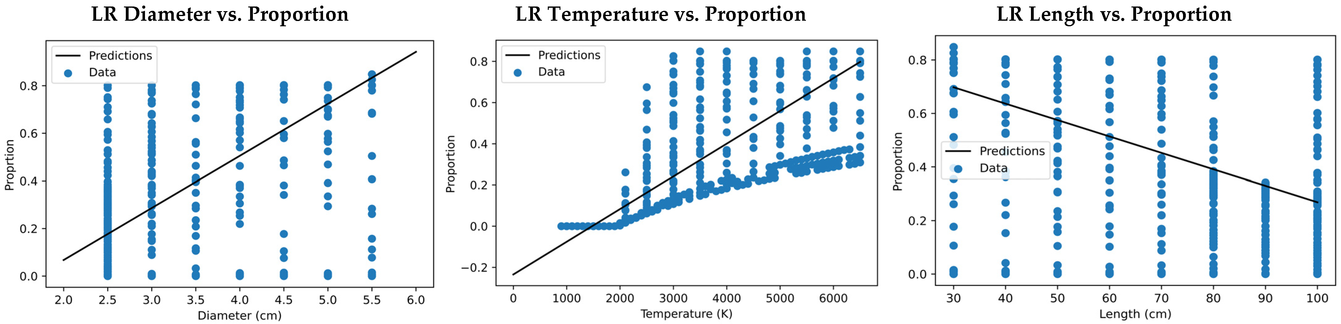
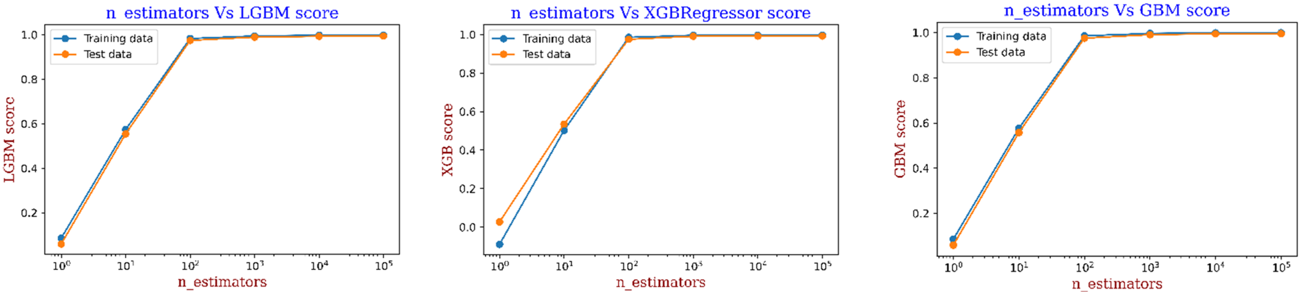
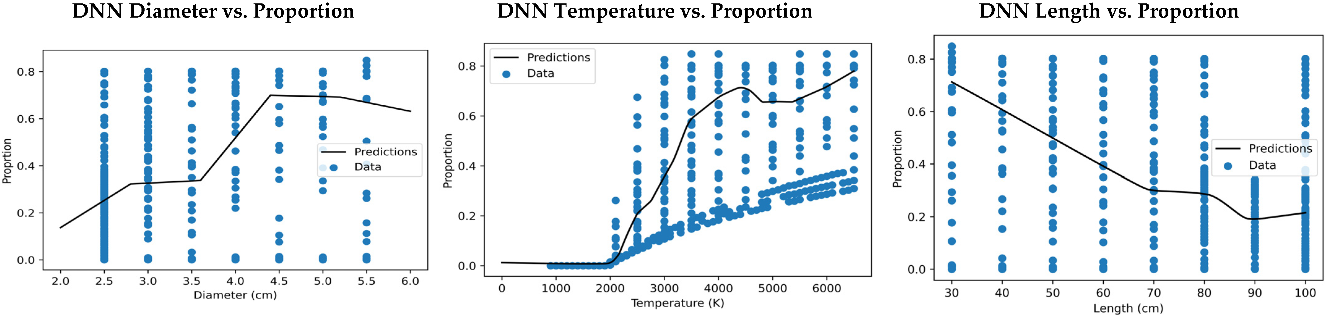
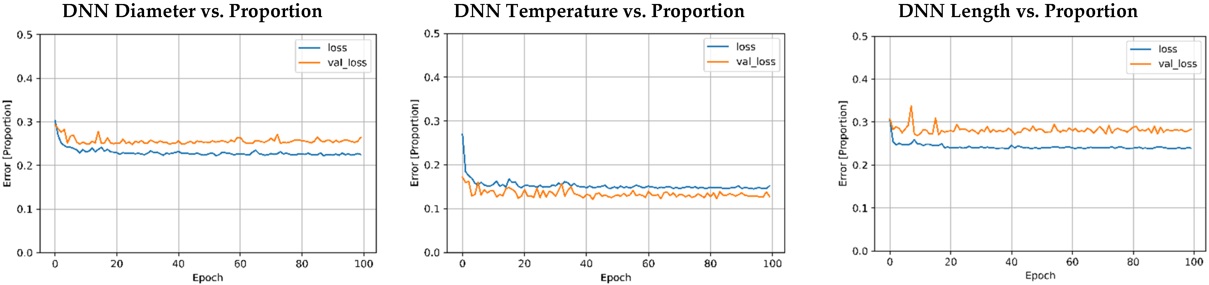
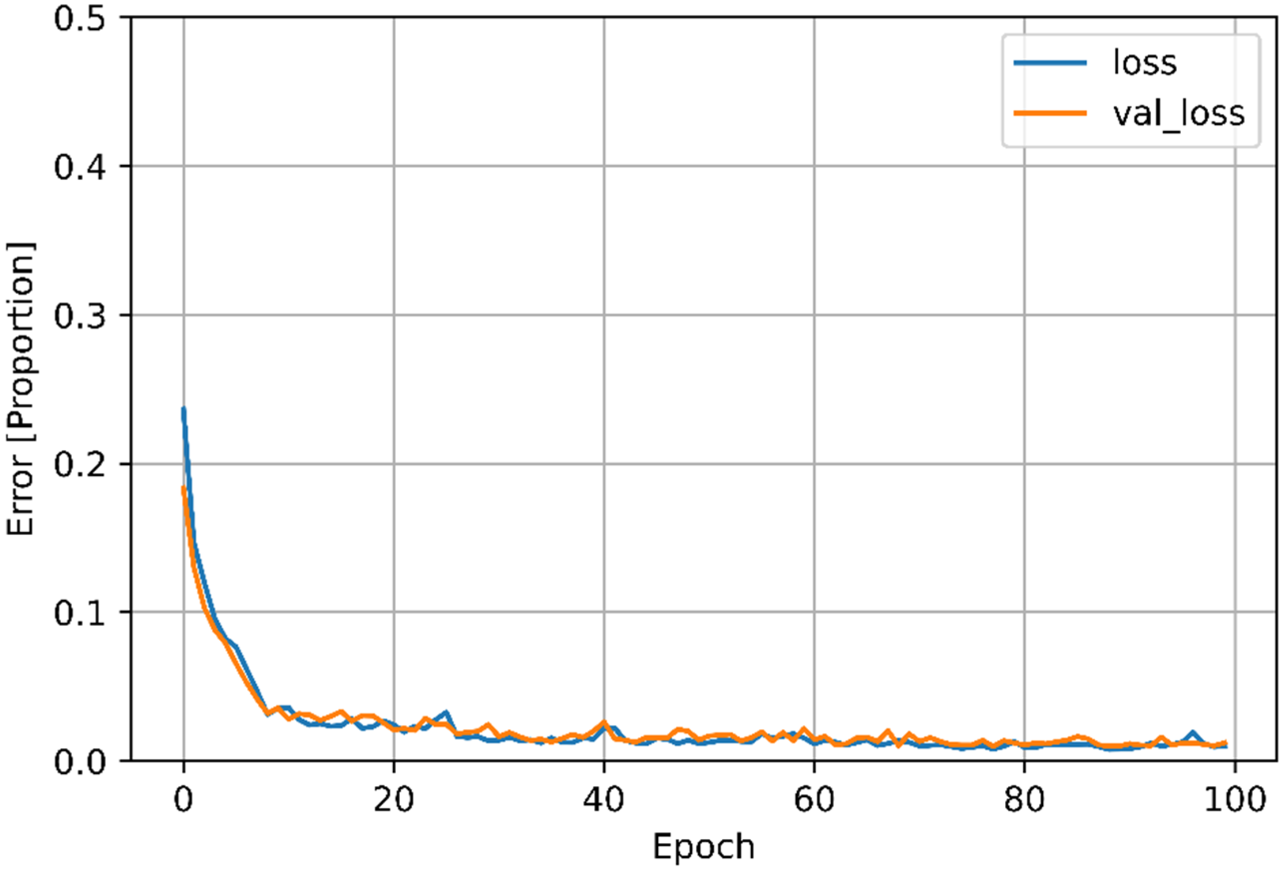
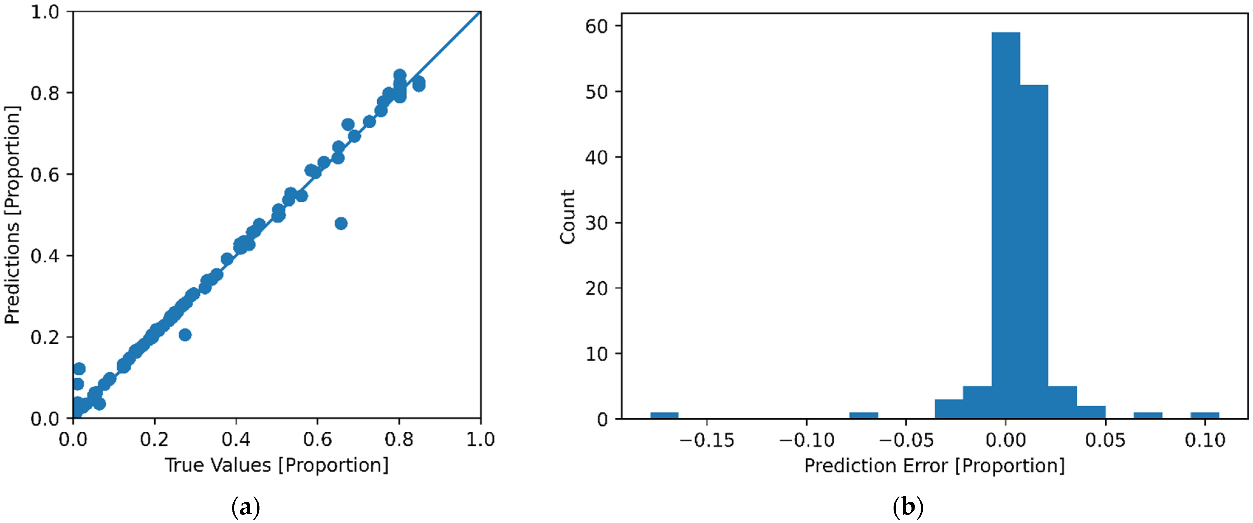
A dataset of 644 CFD modeling iterations containing three different input variables and one output variable was used to train six different ML models. The best ML model to predict the proportion of plasma flame within an EMIPG reactor was found to be the DNN model followed closely by the GBR model. The linear regression model proved to add contrast and show the advantages that non-linear ML models have in the accurate modeling of the non-linear and highly variable time-dependent data commonly found in plasma gasification reactors.

In conclusion, ML models can be used to provide accurate prediction algorithms for EMIPG reactors based on CFD solutions. The ML models allow a user who has no experience with CFD software to understand parameters effecting EMIPG reactors. More importantly, calculations that take a long time using the numerical methods in CFD software can be quickly and accurately modeled with ML models. This study demonstrated that, by using the input parameters of the diameter and length of an EMIPG reactor, and the temperature of the initialized plasma flame, the proportion of the EMIPG reactor that has optimal combustion conditions can be estimated.

More broadly, this study aims to demonstrate that CFD solutions can be synthesized with ML algorithms that are able to provide accurate and fast solutions for specific problems. The availability and ease of use of a ML algorithm can allow someone who has no technical experience in the CFD field to derive equivalent results. This allows for more availability of data and, hopefully, faster process improvement regarding sustainable future technologies such as WtE. Additionally, the incorporation of ML models with numerical solutions has the potential to improve overall solution accuracy and better represent the phenomena in real-life WtE systems. Future recommendations following this work include: creating a larger dataset in order to inform ML models, incorporating experimental data into ML datasets, utilizing ML models with other WtE technologies in order to better understand reactor phenomena, and focusing on other ML model predictive parameters within EMIPG and other WtE reactors.

References

1. Klein, T.; Anderegg, W.R. A vast increase in heat exposure in the 21st century is driven by global warming and urban population growth. Sustain. Cities Soc. 2021, 73, 103098. [Google Scholar] [CrossRef]
2. Khan, S.; Anjum, R.; Raza, S.T.; Bazai, N.A.; Ihtisham, M. Technologies for municipal solid waste management: Current status, challenges, and future perspectives. Chemosphere 2021, 288, 132403. [Google Scholar] [CrossRef] [PubMed]
3. Vergara, S.E.; Tchobanoglous, G. Municipal Solid Waste and the Environment: A Global Perspective. Annu. Rev. Environ. Resour. 2012, 37, 277–309. [Google Scholar] [CrossRef]
4. Johnstone, N.; Labonne, J. Generation of Household Solid Waste in OECD Countries: An Empirical Analysis Using Macroeconomic Data. Land Econ. 2004, 80, 529–538. [Google Scholar] [CrossRef]
5. Ye, Y.; Ngo, H.H.; Guo, W.; Chang, S.W.; Nguyen, D.D.; Varjani, S.; Ding, A.; Bui, X.-T.; Nguyen, D.P. Bio-membrane based integrated systems for nitrogen recovery in wastewater treatment: Current applications and future perspectives. Chemosphere 2021, 265, 129076. [Google Scholar] [CrossRef]
6. Shah, A.V.; Srivastava, V.K.; Mohanty, S.S.; Varjani, S. Municipal solid waste as a sustainable resource for energy production: State-of-the-art review. J. Environ. Chem. Eng. 2021, 9, 105717. [Google Scholar] [CrossRef]
7. Mian, M.; Zeng, X.; Nasry, A.A.N.B.; Al-Hamadani, S.M.Z.F. Municipal solid waste management in China: A comparative analysis. J. Mater. Cycles Waste Manag. 2017, 19, 1127–1135. [Google Scholar] [CrossRef]
8. Waste Management-Google Books. Available online: https://books.google.com/books?hl=en&lr=&id=wgehDwAAQBAJ&oi=fnd&pg=PR7&ots=O8Uti_dYVB&sig=DswFHMaGfTC_FCJTOMMtzezWjWU#v=onepage&q&f=false (accessed on 23 October 2021).
9. Cheng, H.; Hu, Y. Municipal solid waste (MSW) as a renewable source of energy: Current and future practices in China. Bioresour. Technol. 2010, 101, 3816–3824. [Google Scholar] [CrossRef]
10. National Research Council. Waste Incineration and Public Health; National Academies Press: Washington, DC, USA, 2000.
11. Reviewing National Ambient Air Quality Standards (NAAQS): Scientific and Technical Information|US EPA. Available online: https://www.epa.gov/naaqs (accessed on 6 December 2021).
12. Integrated Solid Waste Management: A Lifecycle Inventory: A Lifecycle Inventory, White, P.R.; Franke, M.P. Hindle-Google Books. Available online: https://books.google.com/books?hl=en&lr=&id=QzqdWOOymToC&oi=fnd&pg=PR19&ots=yRIe3AG_cM&sig=VywhICAzeWmdcYwRdghyjF6o17s#v=onepage&q&f=false (accessed on 25 October 2021).
13. Tchobanoglous, G.; Kreith, F. Handbook of Solid Waste Management, 2nd ed.; 2002; Available online: https://www.accessengineeringlibrary.com/content/book/9780071356237 (accessed on 25 October 2021).
14. Rathna, R.; Varjani, S.; Nakkeeran, E. Recent developments and prospects of dioxins and furans remediation. J. Environ. Manag. 2018, 223, 797–806. [Google Scholar] [CrossRef]
15. Chanthakett, A.; Arif, M.; Khan, M.; Oo, A.M. Performance assessment of gasification reactors for sustainable management of municipal solid waste. J. Environ. Manag. 2021, 291, 112661. [Google Scholar] [CrossRef]
16. Khan, S.; Galstyan, H.; Bazai, N.A.; Idrees, M. Surface interaction of cadmium and zinc metal ions on Al2O3 nanoparticles in aqueous solution. Int. J. Environ. Anal. Chem. 2020, 1–18. [Google Scholar] [CrossRef]
17. Usda. DoDI 4170.11 11 December 2009, Inorporating Change 2, 31 August 2018. Available online: https://apps.osd.mil/sites/DoDIIC/Pages/default.aspx (accessed on 23 November 2021).
18. GAO. United States General Accounting Office. Report to Congressional Requesters Hazardous Waste Dod Efforts to Reduce; Wmte: Manistee, MI, USA, 1989.
19. Chester, D.J. AFIT Scholar Theses and Dissertations Student Graduate Works A Life Cycle Analysis of DOD Expeditionary Waste Management Practices Using Simapro. Available online: https://scholar.afit.edu/etd/2328 (accessed on 25 October 2021).
20. DoD’s Energy Efficiency and Renewable Energy Initiatives. Available online: www.eesi.org (accessed on 23 November 2021).
21. U. Department of Veterans Affairs—Airborne Hazards and B. Pit Exposures, VA Airborne Hazards and Open Burn Pit Registry Quick Reference Sheet. Available online: http://www.publichealth.va.gov/airbornehazards (accessed on 25 October 2021).
22. Dod. Task Force on Energy Systems for Forward/Remote Operating Bases; Dod: Washington, DC, USA, 2016.
23. Military Deployment Periodic Occupational and Environmental Monitoring Summary (POEMS): Camp Al Fallujah and vicinity, Iraq Calendar Years: (2004 to 2011), 2004. Available online: https://phc.amedd.army.mil/PHC%20Resource%20Library/U_IRQ_Fallujah%20POEMS%202004-2011_Public%20Release.pdf (accessed on 22 February 2021).
24. Modi, R.; Al Khalisy, H.; Amzuta, I. Burn Pits Exposure and A Case of Usual Interstitial Pneumonia. Chest 2019, 156, A1259. [Google Scholar] [CrossRef]
25. Jani, N.; Falvo, M.; Sotolongo, A.; Osinubi, O.; Tseng, C.-L.; Rowneki, M.; Montopoli, M.; Morley, S.; Mitchell, V.; Helmer, D. Self-Reports of Constrictive Bronchiolitis Among Service Members Participating in the Veterans Administration and Department of Defense Airborne Hazards and Open Burn Pit Registry. Chest 2017, 152, A822. [Google Scholar] [CrossRef]
26. Meier, A.; Shah, M.; Engeling, K.; Quinn, K. Demonstration of Plasma Assisted Waste Conversion to Gas. Int. Conf. Environ. Syst. 2019, 1–13. Available online: https://ttu-ir.tdl.org/handle/2346/84884 (accessed on 22 February 2021).
27. Chen, C.; Chen, J.; Fang, R.; Ye, F.; Yang, Z.; Wang, Z.; Shi, F.; Tan, W. What medical waste management system may cope With COVID-19 pandemic: Lessons from Wuhan. Resour. Conserv. Recycl. 2021, 170, 105600. [Google Scholar] [CrossRef]
28. Sebastian, R.; Louis, J. Understanding waste management at airports: A study on current practices and challenges based on literature review. Renew. Sustain. Energy Rev. 2021, 147, 111229. [Google Scholar] [CrossRef]
29. Erdogan, A.A.; Yilmazoglu, M.Z. Plasma gasification of the medical waste. Int. J. Hydrog. Energy 2021, 46, 29108–29125. [Google Scholar] [CrossRef]
30. Sanlisoy, A.; Carpinlioglu, M. A review on plasma gasification for solid waste disposal. Int. J. Hydrog. Energy 2017, 42, 1361–1365. [Google Scholar] [CrossRef]
31. Perkins, G. Production of electricity and chemicals using gasification of municipal solid wastes. Waste Biorefinery 2020, 3–39. [Google Scholar] [CrossRef]
32. Blaisi, N.I.; Roessler, J.G.; Watts, B.E.; Paris, J.; Ferraro, C.C.; Townsend, T.G. Construction material properties of high temperature arc gasification slag as a portland cement replacement. J. Clean. Prod. 2018, 196, 1266–1272. [Google Scholar] [CrossRef]
33. Sekiguchi, H.; Orimo, T. Gasification of polyethylene using steam plasma generated by microwave discharge. Thin Solid Film. 2004, 457, 44–47. [Google Scholar] [CrossRef]
34. Dharmaraj, S.; Ashokkumar, V.; Pandiyan, R.; Munawaroh, H.S.H.; Chew, K.W.; Chen, W.-H.; Ngamcharussrivichai, C. Pyrolysis: An effective technique for degradation of COVID-19 medical wastes. Chemosphere 2021, 275, 130092. [Google Scholar] [CrossRef] [PubMed]
35. Pintsuk, G.; Hasegawa, A. Tungsten as a Plasma-Facing Material. In Comprehensive Nuclear Materials; Elsevier BV: Amsterdam, The Netherlands, 2020; pp. 19–53. [Google Scholar]
36. Sedej, O.; Mbonimpa, E. CFD Modeling of a Lab-Scale Microwave Plasma Reactor for Waste-to-Energy Applications: A Review. Gases 2021, 1, 133–147. [Google Scholar] [CrossRef]
37. Delikonstantis, E.; Sturm, G.; Stankiewicz, A.I.; Bosmans, A.; Scapinello, M.; Dreiser, C.; Lade, O.; Brand, S.; Stefanidis, G. Biomass gasification in microwave plasma: An experimental feasibility study with a side stream from a fermentation reactor. Chem. Eng. Process. Process. Intensif. 2019, 141, 107538. [Google Scholar] [CrossRef]
38. Ho, G.S.; Faizal, H.M.; Ani, F.N. Microwave induced plasma for solid fuels and waste processing: A review on affecting factors and performance criteria. Waste Manag. 2017, 69, 423–430. [Google Scholar] [CrossRef]
39. Uhm, H.S.; Na, Y.H.; Hong, Y.C.; Shin, D.H.; Cho, C.H. Production of hydrogen-rich synthetic gas from low-grade coals by microwave steam-plasmas. Int. J. Hydrog. Energy 2014, 39, 4351–4355. [Google Scholar] [CrossRef]
40. Hong, Y.C.; Lee, S.J.; Shin, D.H.; Kim, Y.J.; Lee, B.J.; Cho, S.Y.; Chang, H.S. Syngas production from gasification of brown coal in a microwave torch plasma. Energy 2012, 47, 36–40. [Google Scholar] [CrossRef]
41. Ariza, C.; Casado, C.; Wang, R.-Q.; Adams, E.E.; Marugán, J. Comparative Evaluation of OpenFOAM and ANSYS® Fluent for the Modeling of Annular Reactors. Chem. Eng. Technol. 2018, 41, 1473–1483. [Google Scholar] [CrossRef]
42. Xia, H.; Tucker, P.; Dawes, W. Level sets for CFD in aerospace engineering. Prog. Aerosp. Sci. 2010, 46, 274–283. [Google Scholar] [CrossRef]
43. Wang, R.-Q.; Law, A.W.-K.; Adams, E.E. Large-Eddy Simulation (LES) of settling particle cloud dynamics. Int. J. Multiph. Flow 2014, 67, 65–75. [Google Scholar] [CrossRef]
44. Wang, S.; Lu, H.; Zhao, F.; Liu, G. CFD studies of dual circulating fluidized bed reactors for chemical looping combustion processes. Chem. Eng. J. 2014, 236, 121–130. [Google Scholar] [CrossRef]
45. Silva, V.B.R.E.; Cardoso, J. Introduction and overview of using computational fluid dynamics tools. In Computational Fluid Dynamics Applied to Waste-to-Energy Processes; Elsevier BV: Amsterdam, The Netherlands, 2020; pp. 3–28. [Google Scholar]
46. Reactor Design & Simulation|Ansys. Available online: https://www.ansys.com/solutions/solutions-by-industry/materials-and-chemical-processing/reactor-design (accessed on 22 February 2021).
47. Couto, N.; Silva, V.; Bispo, C.; Rouboa, A. From laboratorial to pilot fluidized bed reactors: Analysis of the scale-up phenomenon. Energy Convers. Manag. 2016, 119, 177–186. [Google Scholar] [CrossRef]
48. Silva, V.B.R.E.; Cardoso, J. How to approach a real CFD problem—A decision-making process for gasification. In Computational Fluid Dynamics Applied to Waste-to-Energy Processes; Elsevier BV: Amsterdam, The Netherlands, 2020; pp. 29–83. [Google Scholar]
49. About Ansys. Available online: https://www.ansys.com/about-ansys (accessed on 22 February 2021).
50. Thompson, M.K.; Thompson, J.M. Introduction to ANSYS and Finite Element Modeling. In ANSYS Mechanical APDL for Finite Element Analysis; Elsevier BV: Amsterdam, The Netherlands, 2017; pp. 1–9. [Google Scholar]
51. Tao, L.; Dongmei, Z. Numeric simulation and analysis of H2-O2 premixed combustion based on OpenFOAM. In Proceedings of the 2012 IEEE Symposium on Robotics and Applications (ISRA), Kuala Lumpur, Malaysia, 3–5 June 2012; pp. 27–30. [Google Scholar]
52. OpenFOAM. Available online: https://www.openfoam.com/ (accessed on 18 May 2021).
53. Alrashed, A.A.; Gharibdousti, M.S.; Goodarzi, M.; de Oliveira, L.R.; Safaei, M.R.; Filho, E.B. Effects on thermophysical properties of carbon based nanofluids: Experimental data, modelling using regression, ANFIS and ANN. Int. J. Heat Mass Transf. 2018, 125, 920–932. [Google Scholar] [CrossRef]
54. Vinuesa, R.; Brunton, S.L. The Potential of Machine Learning to Enhance Computational Fluid Dynamics. arXiv 2021, arXiv:2110.02085. [Google Scholar]
55. Pandey, D.S.; Das, S.; Pan, I.; Leahy, J.J.; Kwapinski, W. Artificial neural network based modelling approach for municipal solid waste gasification in a fluidized bed reactor. Waste Manag. 2016, 58, 202–213. [Google Scholar] [CrossRef] [Green Version]
56. Puig-Arnavat, M.; Hernández-Pérez, J.A.; Bruno, J.C.; Coronas, A. Artificial neural network models for biomass gasification in fluidized bed gasifiers. Biomass- Bioenergy 2013, 49, 279–289. [Google Scholar] [CrossRef]
57. Ramos, A.; Rouboa, A. Life cycle thinking of plasma gasification as a waste-to-energy tool: Review on environmental, economic and social aspects. Renew. Sustain. Energy Rev. 2021, 153, 111762. [Google Scholar] [CrossRef]
58. Lin, K.; Lin, Y.-C.; Hsiao, Y.-H. Microwave plasma studies of Spirulina algae pyrolysis with relevance to hydrogen production. Energy 2014, 64, 567–574. [Google Scholar] [CrossRef]
59. Vecten, S.; Wilkinson, M.; Martin, A.; Dexter, A.; Bimbo, N.; Dawson, R.; Herbert, B. Experimental study of steam and carbon dioxide microwave plasma for advanced thermal treatment application. Energy 2020, 207, 118086. [Google Scholar] [CrossRef]
60. Vecten, S.; Wilkinson, M.; Bimbo, N.; Dawson, R.; Herbert, B. Experimental investigation of the temperature distribution in a microwave-induced plasma reactor. Fuel Process. Technol. 2021, 212, 106631. [Google Scholar] [CrossRef]
61. Yoon, S.J.; Lee, J.G. Syngas Production from Coal through Microwave Plasma Gasification: Influence of Oxygen, Steam, and Coal Particle Size. Energy Fuels 2011, 26, 524–529. [Google Scholar] [CrossRef]
62. Yoon, S.J.; Yun, Y.M.; Seo, M.W.; Kim, Y.K.; Ra, H.W.; Lee, J.-G. Hydrogen and syngas production from glycerol through microwave plasma gasification. Int. J. Hydrog. Energy 2013, 38, 14559–14567. [Google Scholar] [CrossRef]
63. Shin, D.H.; Hong, Y.C.; Lee, S.J.; Kim, Y.J.; Cho, C.H.; Ma, S.H.; Chun, S.M.; Lee, B.J.; Uhm, H.S. A pure steam microwave plasma torch: Gasification of powdered coal in the plasma. Surf. Coat. Technol. 2013, 228, S520–S523. [Google Scholar] [CrossRef]
64. Su, L.; Kumar, R.; Ogungbesan, B.; Sassi, M. Experimental investigation of gas heating and dissociation in a microwave plasma torch at atmospheric pressure. Energy Convers. Manag. 2014, 78, 695–703. [Google Scholar] [CrossRef]
65. Tsai, C.-H.; Chen, K.-T. Production of hydrogen and nano carbon powders from direct plasmalysis of methane. Int. J. Hydrog. Energy 2009, 34, 833–838. [Google Scholar] [CrossRef]
66. Wang, Y.-F.; You, Y.-S.; Tsai, C.-H.; Wang, L.-C. Production of hydrogen by plasma-reforming of methanol. Int. J. Hydrog. Energy 2010, 35, 9637–9640. [Google Scholar] [CrossRef]
67. Sturm, G.S.J.; Muñoz, A.N.; Aravind, P.V.; Stefanidis, G. Microwave-Driven Plasma Gasification for Biomass Waste Treatment at Miniature Scale. IEEE Trans. Plasma Sci. 2016, 44, 670–678. [Google Scholar] [CrossRef] [Green Version]
68. Hrycak, B.; Czylkowski, D.; Miotk, R.; Dors, M.; Jasinski, M.; Mizeraczyk, J. Application of atmospheric pressure microwave plasma source for hydrogen production from ethanol. Int. J. Hydrog. Energy 2014, 39, 14184–14190. [Google Scholar] [CrossRef]
69. Su, X.; Jin, H.; Guo, L.; Guo, S.; Ge, Z. Experimental study on Zhundong coal gasification in supercritical water with a quartz reactor: Reaction kinetics and pathway. Int. J. Hydrog. Energy 2015, 40, 7424–7432. [Google Scholar] [CrossRef]
70. ANSYS FLUENT 12.0 Theory Guide-17.4 Energy Equation. Available online: https://www.afs.enea.it/project/neptunius/docs/fluent/html/th/node353.htm (accessed on 23 November 2021).
71. ANSYS FLUENT 12.0 Theory Guide-1 Basic Fluid Flow. Available online: https://www.afs.enea.it/project/neptunius/docs/fluent/html/th/node9.htm (accessed on 23 November 2021).
72. ANSYS FLUENT 12.0 Theory Guide-4.4.1 Standard-Model. Available online: https://www.afs.enea.it/project/neptunius/docs/fluent/html/th/node58.htm (accessed on 4 November 2021).
73. The Python Language Reference—Python 3.10.4 Documentation. Available online: https://docs.python.org/3/reference/ (accessed on 31 January 2022).
74. User Guide—Pandas 1.4.1 Documentation. Available online: https://pandas.pydata.org/docs/user_guide/index.html (accessed on 27 March 2022).
75. McKinney, W. Data Structures for Statistical Computing in Python. Proc. Python Sci. Conf. 2010, 56–61. [Google Scholar] [CrossRef] [Green Version]
76. Pedregosa, F. Scikit-learn: Machine Learning in Python Gaël Varoquaux Bertrand Thirion Vincent Dubourg Alexandre Passos PEDREGOSA, VAROQUAUX, GRAMFORT ET AL. Matthieu Perrot. J. Mach. Learn. Res. 2011, 12, 2825–2830. [Google Scholar]
77. Developers, T. TensorFlow. Available online: https://zenodo.org/record/5949169/export/schemaorg_jsonld#.YkRbPzURVPY (accessed on 31 January 2022).
78. sklearn.linear_model.LinearRegression-scikit-learn 1.0.1 documentation. Available online: https://scikit-learn.org/stable/modules/generated/sklearn.linear_model.LinearRegression.html (accessed on 6 November 2021).
79. Ma, H.; Yang, X.; Mao, J.; Zheng, H. The Energy Efficiency Prediction Method Based on Gradient Boosting Regression Tree. In Proceedings of the 2018 2nd IEEE Conference on Energy Internet and Energy System Integration (EI2), Beijing, China, 20–22 October 2018; pp. 1–9. [Google Scholar]
80. Xue, P.; Lei, Y.; Li, Y. Research and prediction of Shanghai-Shenzhen 20 Index Based on the Support Vector Machine Model and Gradient Boosting Regression Tree. In Proceedings of the 2020 International Conference on Intelligent Computing, Automation and Systems (ICICAS), Chongqing, China, 11–13 December 2020; pp. 58–62. [Google Scholar] [CrossRef]
81. Huaiyu, L.; Hongli, W.; Guanmin, L.; Shuangmei, L.; Jialiang, G. Study on Urban Wastewater Discharge Forecasting and Influence Factors Analysis Based on Stochastic Gradient Regression. In Proceedings of the 2009 Third International Symposium on Intelligent Information Technology Application, Nanchang, China, 21–22 November 2009; pp. 483–486. [Google Scholar] [CrossRef]
82. Biomass Gasification and Pyrolysis: Practical Design and Theory-Prabir Basu-Google Books. Available online: https://books.google.com/books?hl=en&lr=&id=QSypbUSdkikC&oi=fnd&pg=PP1&ots=VhYs1aEqi7&sig=a_zyESQtIQG8vbKXVM8knPL1fNs#v=onepage&q&f=false (accessed on 7 November 2021).
83. Baruah, D. Modeling of biomass gasification: A review. Renew. Sustain. Energy Rev. 2014, 39, 806–815. [Google Scholar] [CrossRef]
84. Kartal, F.; Özveren, U. A deep learning approach for prediction of syngas lower heating value from CFB gasifier in Aspen plus®. Energy 2020, 209, 118457. [Google Scholar] [CrossRef]
85. Ozonoh, M.; Oboirien, B.; Higginson, A.; Daramola, M. Performance evaluation of gasification system efficiency using artificial neural network. Renew. Energy 2020, 145, 2253–2270. [Google Scholar] [CrossRef]
86. Shahbaz, M.; Taqvi, S.A.; Loy, A.C.M.; Inayat, A.; Uddin, F.; Bokhari, A.; Naqvi, S.R. Artificial neural network approach for the steam gasification of palm oil waste using bottom ash and CaO. Renew. Energy 2019, 132, 243–254. [Google Scholar] [CrossRef]
87. ANSYS FLUENT 12.0 User’s Guide-26.13.1 Monitoring Residuals. Available online: https://www.afs.enea.it/project/neptunius/docs/fluent/html/ug/node812.htm (accessed on 23 November 2021).
88. Arpia, A.A.; Nguyen, T.-B.; Chen, W.-H.; Dong, C.-D.; Ok, Y.S. Microwave-assisted gasification of biomass for sustainable and energy-efficient biohydrogen and biosyngas production: A state-of-the-art review. Chemosphere 2021, 287, 132014. [Google Scholar] [CrossRef]
89. Li, J.; Tao, J.; Yan, B.; Jiao, L.; Chen, G.; Hu, J. Review of microwave-based treatments of biomass gasification tar. Renew. Sustain. Energy Rev. 2021, 150, 111510. [Google Scholar] [CrossRef]
Figure 1. Numerical model geometry and meshing structure for 5.50 cm × 100 cm EMIPG reactor.
Energies 15 02559 g001
Figure 2. DNN model structure used to predict the proportion of reactor >2000 K in an EMIPG reactor.
Energies 15 02559 g002
Figure 3. CFD solution for an EMIPG reactor with contour diagram and scaled residuals.
Energies 15 02559 g003
Figure 4. Pair plot of the dataset from the CFD model. Units: Temperature (K), Diameter (cm), Length (cm).
Energies 15 02559 g004
Figure 5. Correlation matrix of the dataset provided by CFD simulations.
Energies 15 02559 g005
Figure 6. Input parameter vs. proportion with linear regression prediction and dataset (Units: Diameter (cm), Temperature (K), and Length (cm)).
Energies 15 02559 g006
Figure 7. Linear regression model with all input parameters, 100 epochs.
Energies 15 02559 g007
Figure 8. n_estimators vs. GBM models: LightGBM (LGBM), XGRegressor Score, and GBM respectively, from left to right.
Energies 15 02559 g008
Figure 9. DNN model for diameter, temperature, and length predictions vs. dataset.
Energies 15 02559 g009
Figure 10. DNN model for diameter, temperature, and length error for 100 epochs.
Energies 15 02559 g010
Figure 11. DNN model of all inputs over 100 epochs.
Energies 15 02559 g011
Figure 12. (a) True value vs. DNN prediction. (b) Histogram of DNN prediction error.
Energies 15 02559 g012