Influence of Geometrical Parameters on the Shape of the Cycloidal Function Curve of a Fan with a Cycloidal Rotor

Abstract

Even though the cycloidal rotor concept has been around for almost a century, it is still not as popular as it should be. Most often it is used to propel unmanned aerial vehicles or sea-going ships, or it is applied as a river- or sea-energy converter. Despite the possibility of directing the flow by changing the inclination angle of blades and the possibility of working in both directions, there are no scientific studies on the use of the concept in HVAC (heat, ventilation and air conditioning). One of the most important elements characterizing the operation of the cycloidal rotor is the cycloidal function describing the change in the angles of the blades during rotation. To properly design a cycloidal rotor for a preferred application, an analysis of the rotor geometrical parameters must be performed and analyzed. This was performed on a four-blade rotor equipped with CLARK Y blades. Using Ansys CFX software, a CFD model of a fan operating with various cycloidal functions was created. The results were compared with the experimental data with the use of the LDA technique. Different velocity profiles were obtained despite the use of cycloidal functions with similar waveforms and small angular differences. This is due to the considerable sensitivity of the cycloidal regulation system to differences in the geometrical sizes that describe it.

1. Introduction

Even though the cycloidal rotor concept is over a century old [1,2], it is still not researched or utilized widely enough despite its advantages. It is most often used in aviation as a form of propulsion for MAVs (micro air vehicles) or UAVs (unmanned air vehicles) [2,3,4] and in the marine sector as a cycloidal propeller for sea-going ships [5]. There are also attempts to use a cycloidal rotor in vertical axis wind turbines (Darrieus) [6] and in a river or offshore energy converters [7,8,9]. Kirsten and Boeing can be considered pioneers of scientific research on using a cycloidal rotor (cyclorotor) as a propulsion for airplanes and ships [10]. One of the most important advantages of this concept is the possibility to immediately change the direction of the thrust. Based on this feature, scientists developed the idea of a cycloplane, i.e., an aircraft powered by two cycloidal rotors. Although the design was characterized by relatively high efficiency, it was not very well received, as it required the use of a huge hub size and a working motor capable of operating in a wide range of rotational speeds.

In the 1920s and 1930s, Strandgren built several cycloidal rotor models and conducted a series of experimental studies [11]. He published an aerodynamic model in which he presented the distribution of forces on the rotor. In the work, the author also presented an assessment of the feasibility of the presented concept.

Wheatley [12] published an aerodynamic theory based on the momentum theory of the blade element. On its basis, he examined the feasibility of the concept of a manned aircraft and assessed that the model presented by them makes it possible to build a vehicle that can hover, rise vertically and move freely in the air. The author noted, that due to the difficulties in constructing such a vehicle, it might have been impossible to make at the time. Together with Windler [13], they built an experimental stand for a four-blade cycloidal rotor equipped with blades with a NACA 0012 profile, which was set in a wind tunnel. The experiments aimed to describe the value and distribution of forces arising on the rotor in the conditions of hover and forward flight. Using the experimental stand, the influence of the blade movement on the rotor operation (force distribution and generation) under conditions of hovering and a forward flight at various rotational speeds were investigated. The occurrence of lateral forces caused by the Magnus effect was described. Thanks to experimental measurements, the relationships concerning the blade profile coefficients and the drag coefficients were determined.

Tanuguchi [2,14,15,16] developed an aerodynamic analysis to determine the hover and forward performance of a cycloidal rotor. Thrust and torque were determined by combining the lift and drag forces acting on each blade section. The authors assumed that only the longitudinal velocities affect the thrust and the rotor torque; their value is constant over the entire blade surface, and the longitudinal speed is not a function of the orbital position of the blade. The value of these velocities is obtained using the momentum theory after applying a correction factor based on the experimental results on the six-bladed cycloidal rotor.

Yun’s research team [17] introduced the concept of a mechanical cycloidal adjustment that made it possible to change the angles of the rotor blades. The authors described the mathematical model on the basis of the individual geometrical quantities of the control system, and the forces generated by the rotor were described. Two-dimensional CFD calculations of the 6-blade NACA 0012 profile rotor were performed and compared with the experimental data. The highest thrust was obtained for the largest amplitude of the rotor blades and the rotational speed.

Hwang’s research team [18] designed and built a model of a cyclocopter powered by four cycloidal rotors (quadrocopter), based on the work of Yun [17,19]. For this purpose, 2D and 3D numerical calculations were performed. The 4-blade NACA 0018 profile rotor, which has been elliptically rounded, was analyzed. The research was aimed at determining the thrust generated by the cyclocopter rotors and their power demand.

Sirohi’s research team [20] conducted tests of a compact cycloidal rotor to determine its applicability in UAVs. The research was to lead to the creation of a fully functional 250 g cyclocopter. The tests were carried out on rotors with a diameter of approx. 15 cm, for which the influence of the number of blades, their angle of inclination and rotational speed were determined. To obtain the approximate performance of the cycloidal rotor, an analytical model based on the theory of the wind turbine was used [12]. The authors obtained a satisfactory agreement between the analytical model and the experimental data and showed that the efficiency of the system largely depends on the design used, as well as the friction between the control elements.

Between 2013 and 2014, the international CROP (Cycloidal Rotor Optimized for Propulsion) project aimed at introducing an innovative cycloidal rotor propulsion system to introduce a new concept for air vehicles, overcoming the traditional limitations of short take-off and landing, including the possibility of hovering [6,21,22,23,24,25].

Xisto’s research team [6] checked the impact of the key geometric parameters of a cycloidal rotor on its operations. The influence of the blade profile, the number of blades, the c/R ratio and the location of the axis of rotation of the blade were investigated. Numerical calculations and parametric analysis were carried out, taking into account the large-scale model of the cyclorotor under hover conditions. Among the analyzed profiles, the authors proposed the NACA 0018 profile as the best. The rotor with the highest power load was a three-blade rotor, but it generated less thrust compared to a four-blade rotor. It has been proposed to use such a configuration when thrust is required more than a power load. In the case of using a six-blade rotor, a significant deterioration in the rotor load and thrust was noticed due to the interference effects between the blades. The influence of the blade pivot point on the rotor operation was analyzed.

Andrisani’s research team [21] tried to determine the optimal angle of inclination of the cycloidal rotor blades to reduce the demand for power at a given thrust. Analytical calculations were carried out to determine the kinematics and basic aerodynamic properties of the rotor. Then, Lagrange optimization was used to determine the best possible range of inclination angles under hover conditions. The results obtained in this way were compared with the data obtained from 2D numerical calculations. The subject of the research was the IAT L3 rotor operating with an amplitude of approx. 40°. The cycloid function determined by Lagrange’s optimization was implemented into the numerical model to determine the aerodynamic properties of the cycloidal rotor and to validate the selected analytical model. Thanks to optimization, the authors obtained a theoretical increase in rotor efficiency by 25%.

Gagnon’s research team [22] investigated the aeroelasticity of a cycloidal rotor under flight conditions. For this purpose, the influence of the number of blades, their thickness and flexibility on the characteristics of the rotor were investigated. Analytical, numerical and experimental calculations were carried out. Three rotors were analyzed, proposed by Yun, IAT32 L3 and proposed by McNabb [26]. For selected rotors, the authors obtained the results of the experiments, which were then compared with the results obtained from the analytical and numerical calculations. The authors concluded that the influence of elasticity on thrust and power is small, while on the performance itself, it is negligible. The gusts of wind have little effect on the strength of the blades, but they largely affect the power and thrust of the rotor.

Benedicts’s research team [27] tried to optimize the cycloidal rotor for MAV using performance measurements. The aim was to determine the influence of rotational speed, amplitude of the blade pitch angle and the number of blades on the operation of the cycloidal rotor. Thrust measurements suggested a lateral force beyond the vertical lift. Optimized rotors were used on two different MAV cyclocopters, two-rotor and four-rotor cyclocopters, which were both hoverable. Control strategies for the position control of the four-rotor cyclocopter were developed and implemented. Detailed parametric studies were carried out to determine the effects of the number of blades, rotational speed and pitch amplitude of the blades. The results showed that the power load and rotor efficiency increased with the use of more blades. Operation of the cyclorotor at higher pitch amplitudes resulted in better efficiency, regardless of the number of blades. Increasing the number of blades increased the slope of the resultant thrust vector concerning the vertical due to the increasing share of the lateral force. The values of vertical and lateral forces generated by the cyclorotor were determined, and the results were confirmed experimentally.

Adams’ research team [28,29] introduced a prototype of a fully flying cyclocopter. A prototype weighing 535 g was built, equipped with two cycloidal rotors and a tail rotor. To make flight possible, a novel centrifugal-driven mechanism was developed. A control strategy was implemented which made it possible to control the direction of the thrust and its size. The cyclocopter used double cycloidal rotors equipped with four blades with a NACA 0015 profile, 5 cm long. The rotor diameter was 15 cm, and it was the same as its span. The most important element of the MAV was the cycloidal control, which had two servos that could change the position of the regulation about the rotor. This is a significant simplification compared to older solutions, where one servo was used for each blade. To make the structure as light and durable as possible, it was made of carbon fiber. To reduce the weight while maintaining stiffness and durability, the rotor blades consisted of a hollow skeleton made of Delrin over which a mylar foil was stretched. Thanks to this procedure, the weight of one blade was limited to 5 g. The cyclorotor was powered by a single 100 W motor powered by an 850 mAh battery. The mechanism used allowed the rotor to work based on inclination angles with a different course. Thanks to this, it was possible to direct and change the size of the thrust. As can be seen, there is no systematic research on the possibility and use of such a solution in stationary applications, e.g., in HVAC (heat, ventilation and air conditioning) systems. The presented article will show the influence of changes in various geometrical parameters of the mechanical cycloidal control on the shape of the function curve. The referenced values will be characteristic only for a fan with a specific size of the cycloidal rotor. The aim is to show only the general impact of geometrical quantities, which in a way will show the problem of calibration and the level of complexity of mechanical cycloidal regulation.

2. Subject of Investigation

The design of the cycloidal rotor fan (CRF) was based on our own experience and on the design concept most often used in the research. A rather compact size of the four-blade fan impeller was selected [30]. It was decided to make a machine with a radius R = 70 mm and span of 25 cm. Using the c/R ratio, and following the values presented in the literature [6,21,22], it was decided to install the blades with chord c = 50 mm. The fan was placed in the middle of a 4 m long duct. The internal dimensions of the channel were 25 × 25 cm. Rotor was equipped with an asymmetric CLARK Y profile. The optimal pivoting point P selected for the blade (Figure 1b) was located between 35 and 50% [6] of the c length from the blade beginning; the center of the blade was selected for the analyzed variant.

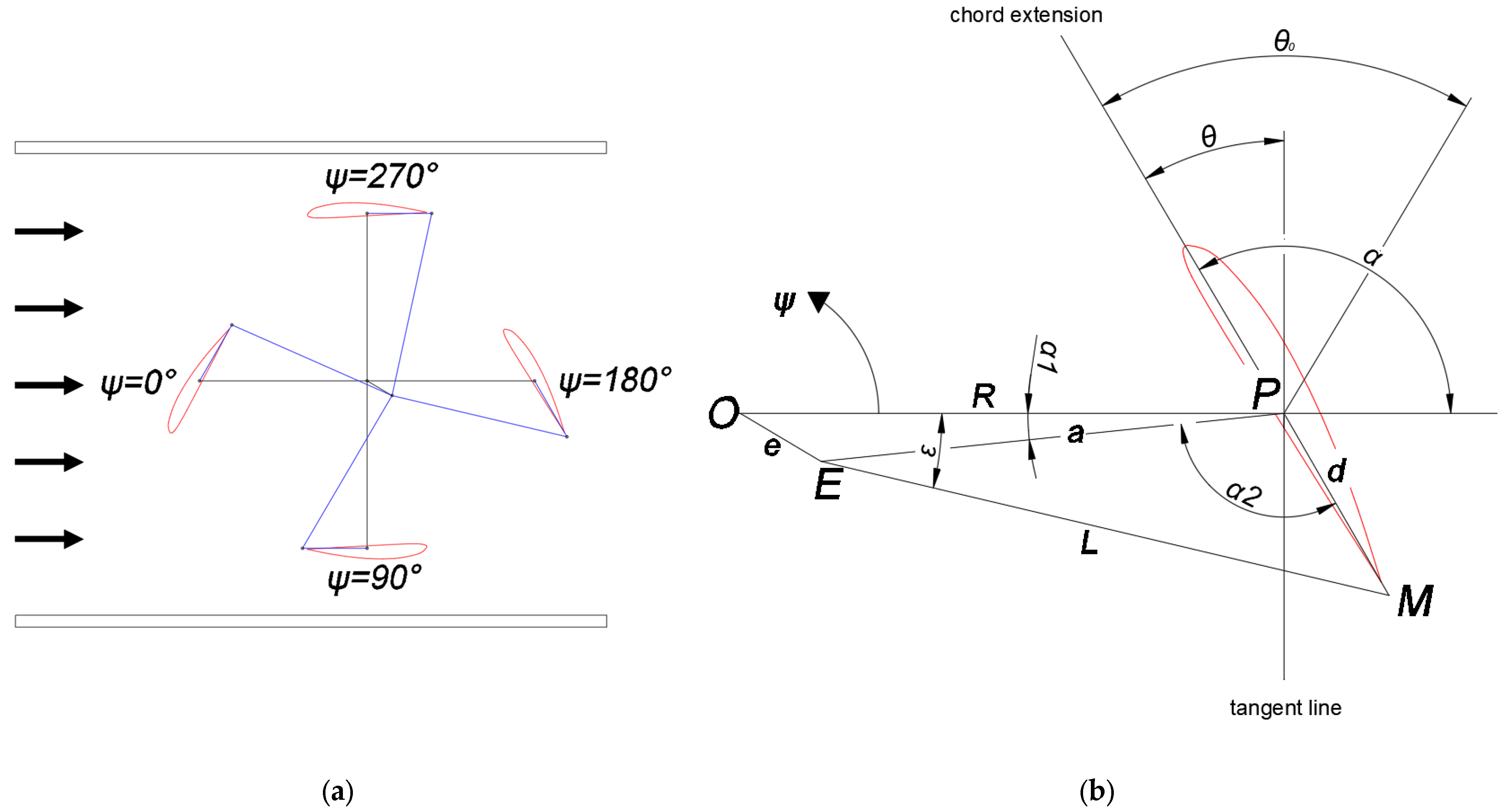
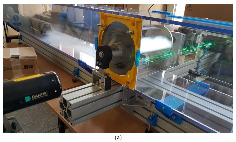
Figure 1a shows a diagram of the analyzed cycloidal rotor with a cycloidal control (marked in blue) placed in the channel [31,32]. The change in the angle of the blade during rotation is described by a certain cycloidal function. For each blade, the function curve should be the same but shifted by an angle of 90°. Due to the imperfections of the structure, it should be noted that these functions vary slightly depending on the blade. The principle of operation of a fan with a cycloidal rotor will be described based on a blade set to position ψ = 0° (Figure 1a). The rotor operation can be divided into 2 stages. The stream is drawn in during the blade rotation from ψ = 0 to 180°, while ejection occurs from ψ = 180 to 0°. The analysis starts from ψ = 0°. In this position, the blade is closest to the top of the channel; its angle of inclination θ should be 0°. By turning in line with the rotation of the ψ rotor, the inclination angle is reduced to the lowest θ value of θ_min. Moving towards the lower part of the tunnel, the inclination angle θ increases to θ = 0°. Due to the operation of the rotor, it is important that the values of the θ at opposite rotor positions (ψ = 0 and 180°) are as close to each other as possible. At higher rotational speeds, the vibrations are increased due to the dynamic unbalance of the rotor [31]

The lowest vibrations and noise would be generated by the rotor, for which the blades in the second rotor part realize the change of θ angles with exactly opposite values. However, due to the mathematical model used [6], the fan size and production capabilities, it is possible to obtain only a similar cycloidal function. In the 2nd part of the rotor, the θ angle increases until it reaches θ_max at the ψ = 27°. When this value is exceeded, the blade reduces θ until it reaches 0 for ψ = 0°.

Figure 1b shows a fragment of the cyclorotor with marked geometrical quantities. Point 0 is the geometrical center of the rotor, point E is the geometrical center of the mechanical cycloidal control moved by angle ε, point P is the blade pivoting point, while M is the point of attachment of the mechanical control gear arm with length L to the blade. Inclination angle θ can be described as in [25]:

$$\theta =\frac{\pi }{2}-\alpha ,$$

(1)

where

$$\alpha ={\alpha }_1+{\alpha }_2.$$

(2)

Summand α₁ is the angle between the rotor radius R and a, while α₂ is the angle between a and the camber line of the blade. The above-mentioned parameter a is the length of the segment between points E and P. The cycloidal control system is shifted by angle ε from the rotor axis. This can be described as

$$a^2= e^2+R^2-2eR\cos \left(\psi +\epsilon +\frac{\pi }{2}\right),$$

(3)

$$\frac{\sin \left({\alpha }_1\right)}{e}=\frac{\cos \left(\psi +\epsilon +\frac{\pi }{2}\right)}{a}$$

(4)

where e is the distance determining the shift between the geometrical center of the rotor and the axis of the control system; ψ determines the current position of the blade on the circle, and ε is the mentioned angle by which the mechanical control is shifted. On the other hand, length L, which is the length of the tension member, can be described as:

$$L=\sqrt{a^2+d^2-2ad\cos \left({\alpha }_2\right)}.$$

(5)

Finally, the dependence of the blade inclination angle θ on its position on the rotor can be described as:

$$\theta =\frac{\pi }{2}-{\sin }^{-1}\left[\frac{e}{a}\cos \left(\psi +\epsilon \right)\right]-{\cos }^{-1}\left[\frac{a^2+d^2-L^2}{2ad}\right].$$

(6)

The above equation shows that for each position of the rotor blade ψ, the value of θ changes only due to a change in the eccentric phase angle ε and shift e because length L and distance d are constant for a given mechanical system.

Equation (5) defines the tension member length L as being the length of the cycloidal gear arm. The last Equation (6) defines the blade inclination angle θ. Based on the above equations, a program was created in the LabVIEW software that enables the creation and optimization of the cycloidal function based on the selection of geometrical parameters.

The values of the geometrical quantities describing the geometry of the cycloidal regulation are presented in

Table 1. Geometric parameters of cycloidal regulation.

Geometrical Parameter	Parameter Value
L	74 mm
d	27 mm
e	13 mm
ε	292°

.

3. Sensitivity Analysis

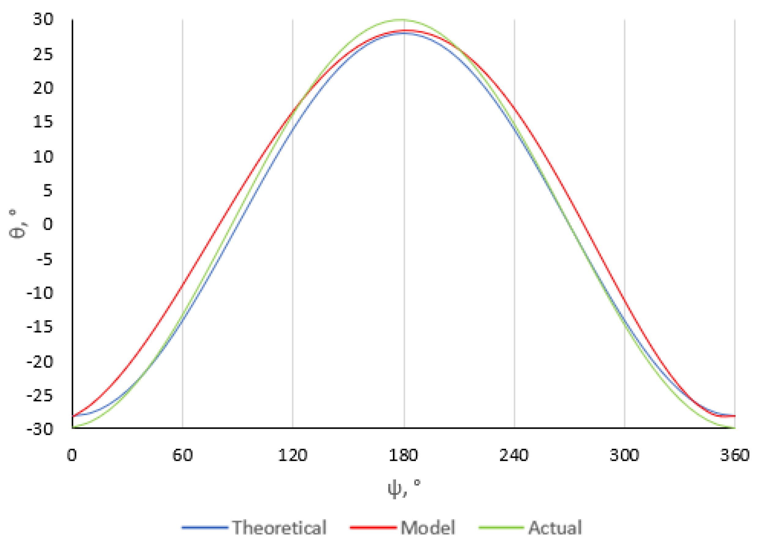
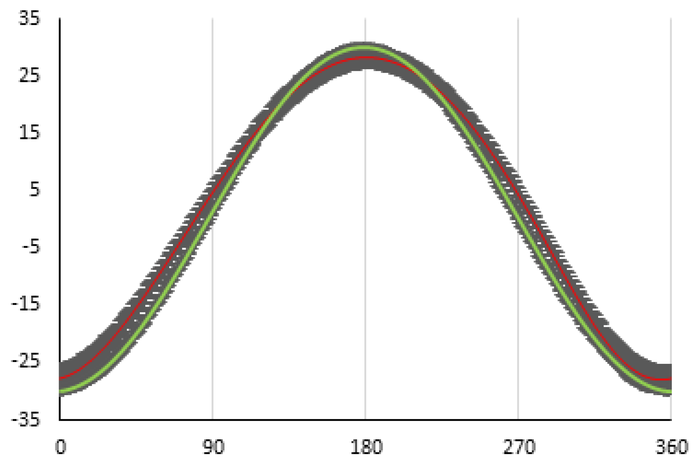
By analyzing the operation of the cycloidal function and the changes in the function values for the rotor under consideration, 3 functions can be determined [32]. Figure 2 below shows a set of example cycloidal function curves plotted for one blade (cf. Figure 1a). The fan working according to the following functions operates with an amplitude of θ₀~60°.

Figure 2 shows the curves illustrating changes in the values of the 3 cycloidal functions under analysis: model, theoretical and actual. The theoretical function is the best to model the cyclorotor work. The fan that changes angle θ according to this function is characterized by the lowest level of vibrations. Furthermore, the angle extreme value and the zero values of the angles are realized in azimuthal positions. For this reason, for each quarter rotation, the change in angle θ is constant. This function is the product of the cosine function and the minimum value of the θ angle.

When designing the cycloidal control, the aim was to set the rotor to the operating mode based on the theoretical function. With the current dimensions of the machine and cycloidal adjustment, it turned out to be impossible due to the inability to make individual adjustment elements with this accuracy. It was necessary to determine the function as close to theoretical as possible, which was obtained with the aforementioned Labview software. The obtained model function was determined as a model, and on its basis, the cycloidal regulation was set up in the experiment.

The geometrical quantities were selected so that the absolute difference in the θ angle of corresponding azimuthal positions was as small as possible. Such a condition enabled a reduction in the vibration level and, thus, an increase in the RPM ranges.

The actual function describes the change in the blade angle measured on the experimental stand. The shape of this function curve, apart from obvious measurement errors, is also influenced by the accuracy of the making, calibration and adjustment.

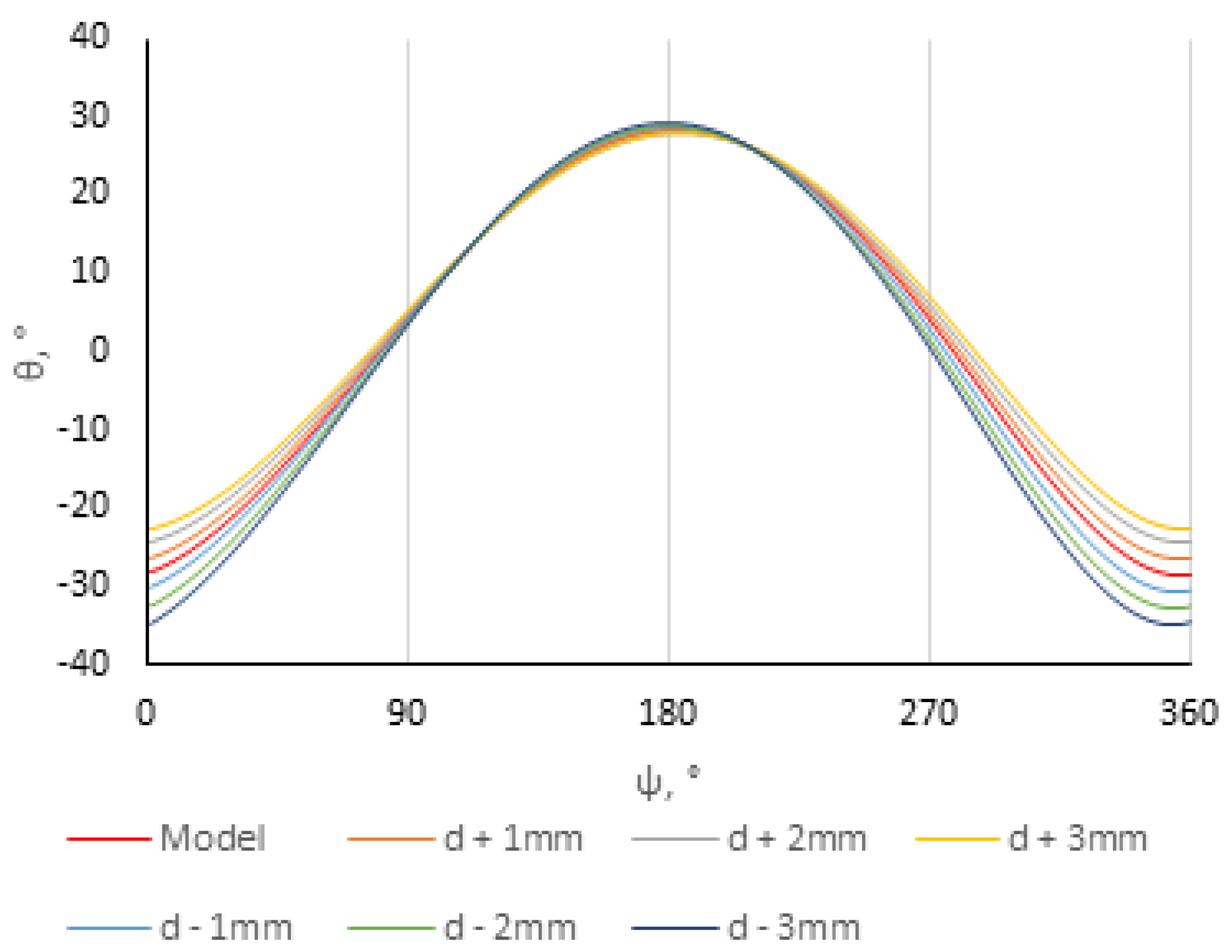
The model function was analyzed by changing various geometrical parameters. The presented curves show the variability of the functions for the mentioned fan size with a cycloidal rotor.

Figure 3 shows the effect of length d on the cycloidal function for the model function with amplitude θ₀ = 60°. The presented changes are shown for a size change of ±1 mm. Changing the value of d alone does not significantly change the value of the blade’s maximum inclination angle (rotation angle ψ = 180°). For such a blade position, the changes do not cause a shift in the maximum value either. An increase in parameter d for a given function involves an increase in the value of the minimum inclination angle by approx. 2°. Shortening distance d will reduce the minimum inclination angle θ by a value similar to the previous case.

Figure 4 shows the influence of the lengthening and shortening of the control gear arm length L on the values of the cycloidal function and, thus, on the shape of the function curve. An increase in length L will increase the minimum angle and lower the value of the maximum inclination angle in the azimuth position. In the case of shortening the tension member, the opposite effect is obtained. Each shift will change the values of the slope by a constant value of about 2°.

During the operation of the fan with a cycloidal rotor, it is possible to change the cycloidal function and, thus, the rotor amplitude θ₀. The change is made by moving the mechanical control away from the geometrical center of the rotor by a certain shift e by angle ε. The effect of an excessive or insufficient shift on the shape of the function curve is substantially similar to the previous cases (cf. Figure 3 and Figure 4). Only the values of the θ_max and θ_min angles of the blades are changed. There are no changes in the angles in blade positions ψ = 90° and 270°. Inaccuracy during the traverse and shifting the center of rotation of E too high will shift the maximum and the minimum θ angle earlier than the azimuthal position (cf. Figure 5b). Shifting by 10° causes a shift of the max/min point by about 5°, which, with larger errors, can significantly increase the lateral force and, as a result, increase the vibration level of the rotor.

The studies of the sensitivity of the cycloid function were in line with the studies carried out by Kiwata and his research team [33]. The authors conducted a wind turbine study to improve efficiency and performed a sensitivity analysis of its geometric parameters. It was found that the amplitude of the blade inclination angles was mainly influenced by the parameters e and d. The increase in amplitude could be achieved by moving the eccentricity point away from the rotor center (increasing the distance e) and shortening the distance between the blade rotation point and the cycloidal control hooking point (shortening the distance e). The results of the analysis also coincide with those determined by Higashi [34] and his research team, who conducted the optimization of geometrical quantities to obtain the highest possible thrust for the cycloidal rotor. The authors found that as the distance e increases, the LW coefficient will increase (it is the ratio of the total lift to mass). Based on the conducted analysis of the aforementioned works, it can be concluded that the sensitivity analysis was carried out correctly and its results coincide with the results of other researchers.

4. Influence of the Geometrical Parameters on the Shape of the Cycloidal Curve

Considering the necessity of measuring individual geometrical quantities that determine the blade inclination angle θ, which is needed to create the model function, the uncertainty analysis was conducted [35]. At first, calibration uncertainties Δdx (arising from the applied measuring instrument) and experimenter uncertainties Δex (arising due to possible readout errors of the experimenter) were determined for L, d, e and ε. The uncertainties are presented in

Table 2. Measuring uncertainties of the mechanical control geometrical parameters.

Measured Quantities x	Calibration Uncertainty Δdx	Experimenter Uncertainty Δex	Standard Calibration Uncertainty Sxd	Standard Experimenter Uncertainty Sxe	Standard Uncertainty Sx
L	0.01 mm	1 mm	0.0058 mm	0.58 mm	0.58 mm
e
d
ε	0.5°	1°	0.29°	0.58°	0.65°

.

Quantities L, d and e were measured using a 0.01 mm caliper, whereas ε was established using a protractor with an accuracy of 0.5°. Due to limited space at the test stand and the structure of the mechanical control, readout errors may arise at the level of 0.5 mm for the caliper and 1° for the protractor. Next, standard uncertainties S_xd, S_xe and S_x due to the rectangular distribution of probability were determined according to the following relation [36]:

$$S_{xd}=\frac{{\Delta }_{d}x}{\sqrt{3}},$$

(7)

$$S_{xe}=\frac{{\Delta }_{d}x}{\sqrt{3}},$$

(8)

$$S_x=\sqrt{{S_{xe}}^2+{S_{xd}}^2}.$$

(9)

The next step in the uncertainty analysis was to determine the standard uncertainty of the inclination angle θ, which according to Equation (6) depends on all the geometrical quantities under consideration: L, d, e and ε. The uncertainty propagation rule was used for this purpose, according to the following Equation:

$$S_y=\sqrt{{\left(\frac{\partial y}{\partial x_i}{S}_{x_i}\right)}^2}.$$

(10)

Considering the structure of Equation (6), partial derivatives for individual quantities are difficult to find analytically due to the degree of complexity. For this reason, they were estimated using the following central difference quotient:

$$f^{\prime }\left(x_0\right)\cong \frac{f\left(x_0+\mathsf{\Delta }x\right)-f\left(x_0-\mathsf{\Delta }x\right)}{2\mathsf{\Delta }x}.$$

(11)

The results of standard uncertainty of composite quantity θ for individual geometrical parameters are shown in Figure 6, Figure 7, Figure 8 and Figure 9.

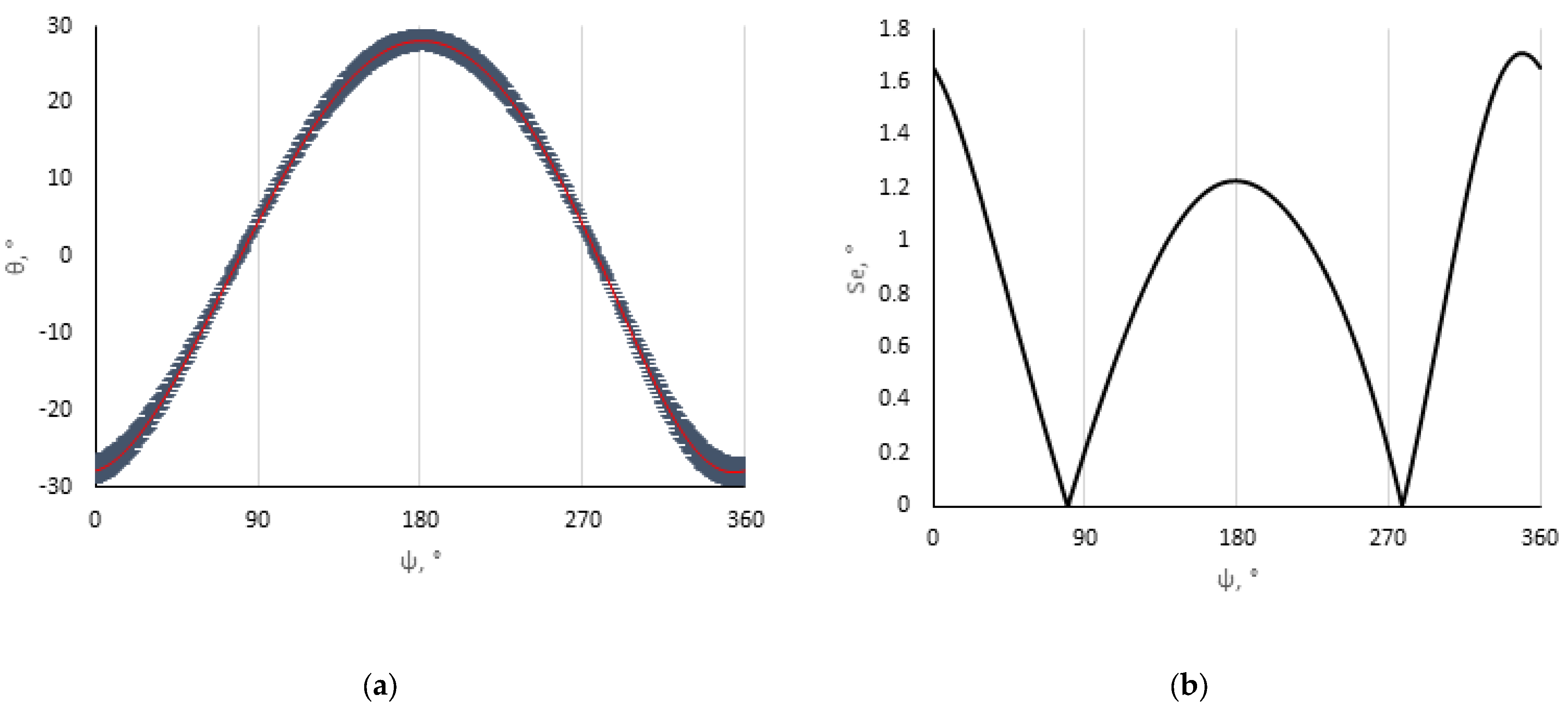
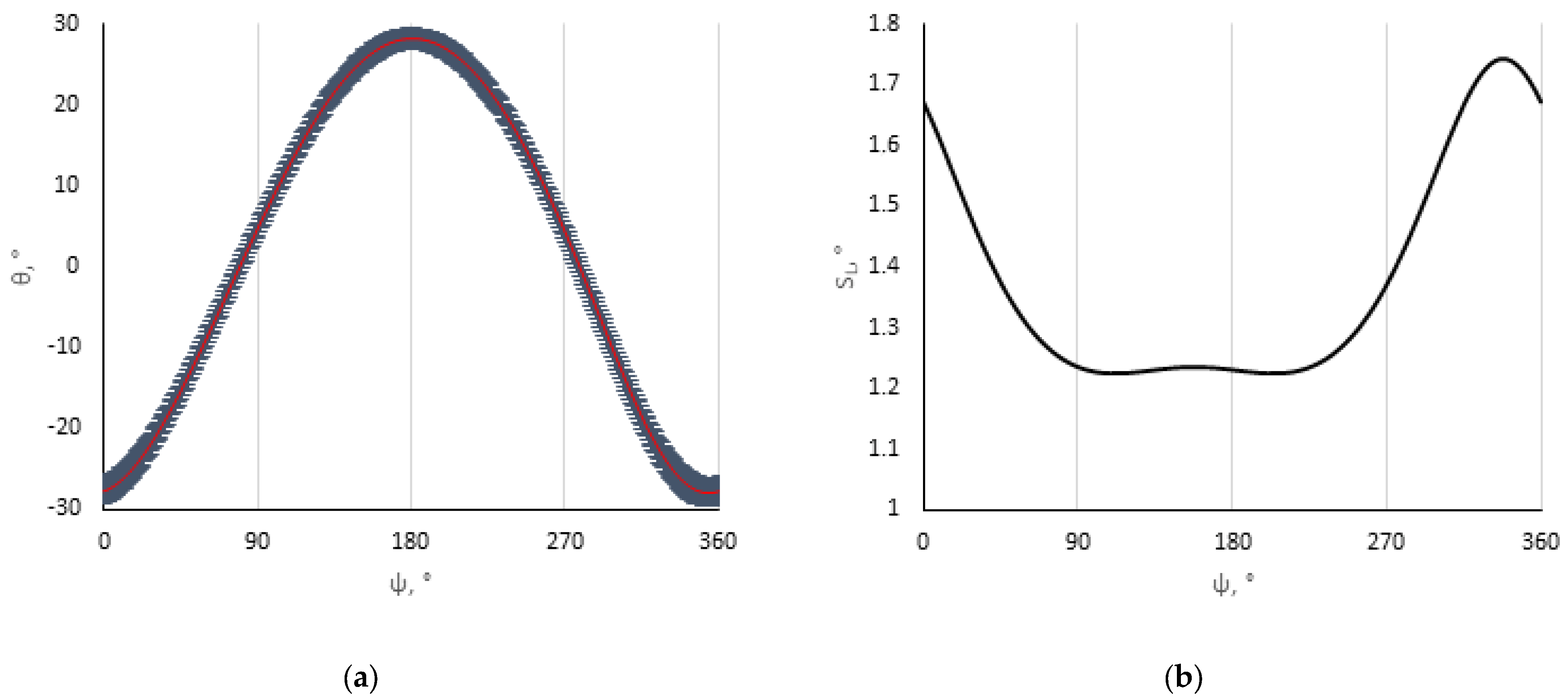
Figure 6 presents the model function together with standard uncertainty due to the measurement of e and the changes in the uncertainty values in relation to the angle of the blade rotation ψ. The highest uncertainties occur for the lowest inclination angles of blades θ, which points to a high correlation between θ and e in this area. The standard measuring uncertainty for θ_min can be established at about ±1.7°. In the case of the blade maximum inclination angle at ψ = 180°, the uncertainty is about ±1.2°. In the case of azimuthal positions, where angle θ = 0° (assumed for ψ = 90 and 270°), the function is independent of the value of e.

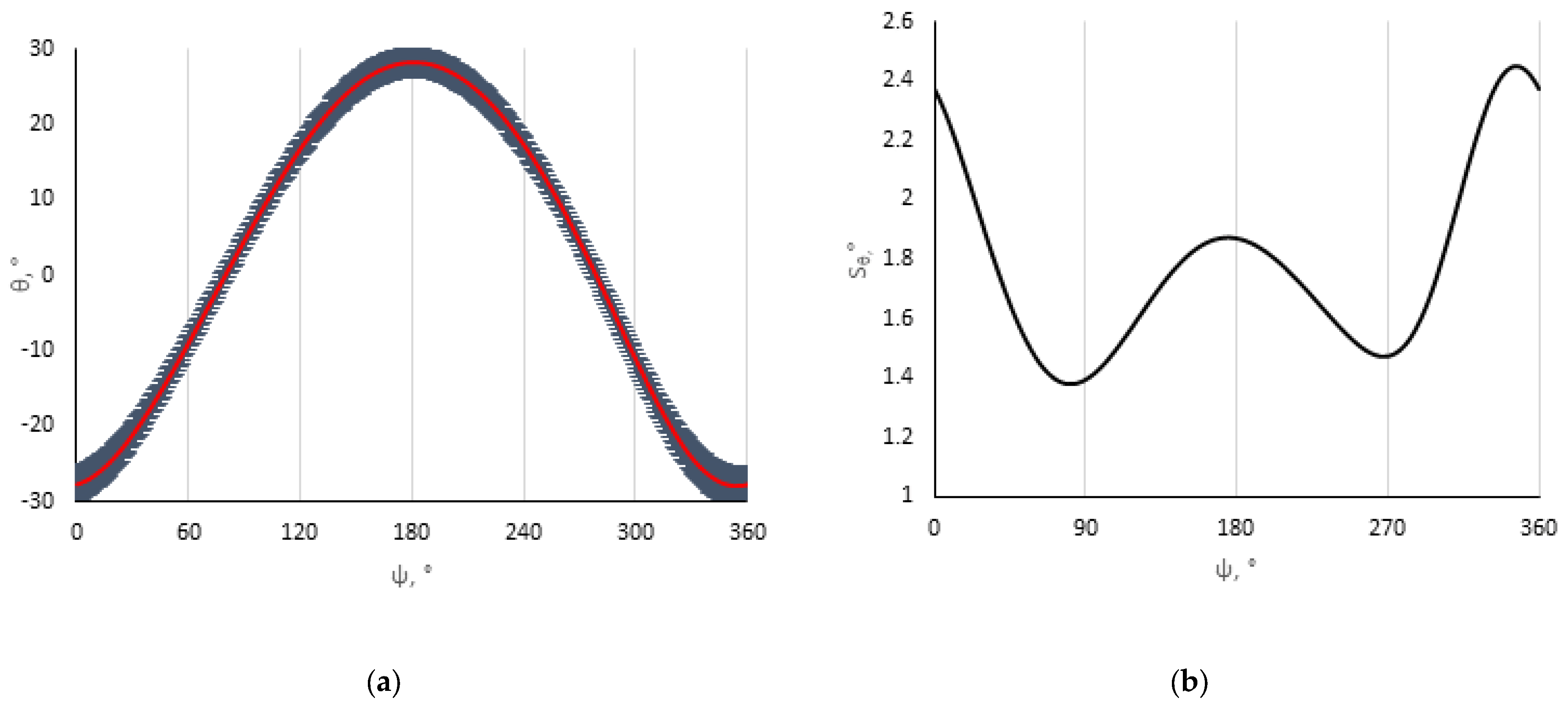
Figure 7 shows the curve illustrating the standard uncertainty of the composite quantity θ due to the standard measuring uncertainty of L and the curve illustrating changes in the uncertainty in relation to the angle of the blade rotation ψ. Such as in the previous case (cf. Figure 6), the highest uncertainties can be observed at θ_min; they have a similar value of about ±1.7°. The lowest standard uncertainties can be observed in the range from ψ = 90° to ψ = 270° during the jet ejection by the rotor. The maximum uncertainty and the sudden drop in its value are related to the shift of the model function.

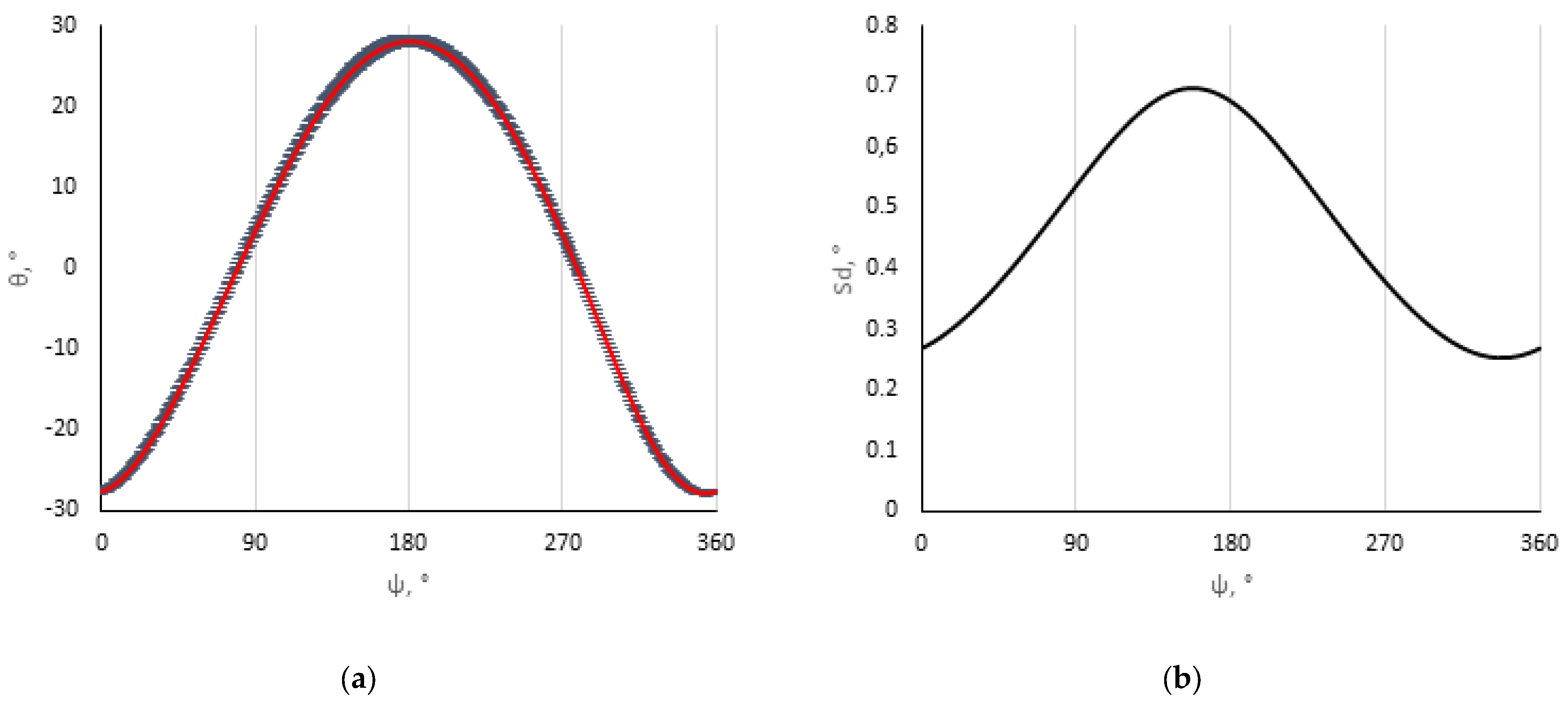
Considering the geometrical parameters measured using a caliper, the lowest standard uncertainty of composite quantity θ was caused by the measurements of d (cf. Figure 8). The highest uncertainty occurred for θ_max. It totals about ±0.7°, and the curve illustrating the changes in its value has a shape similar to the shape of the curve illustrating the cycloidal function itself (Figure 8b).

The smallest standard uncertainty of angle θ was caused by the measurement of ε (Figure 9). The highest value occurred for θ = 0° and totals ±0.35°. For θ_max, standard uncertainty was 0, which indicates that in this point θ is independent of ε.

The standard uncertainty of composite quantity θ being the result of all standard uncertainties of the measurements of L, d, e and ε were determined according to relation (12). The results are presented in Figure 10.

$$S_{\theta }=\sqrt{{\left(\frac{\partial \theta }{\partial e}{S}_e\right)}^2+{\left(\frac{\partial \theta }{\partial L}{S}_L\right)}^2+{\left(\frac{\partial \theta }{\partial d}{S}_d\right)}^2+{\left(\frac{\partial \theta }{\partial \epsilon }{S}_{\epsilon }\right)}^2}.$$

(12)

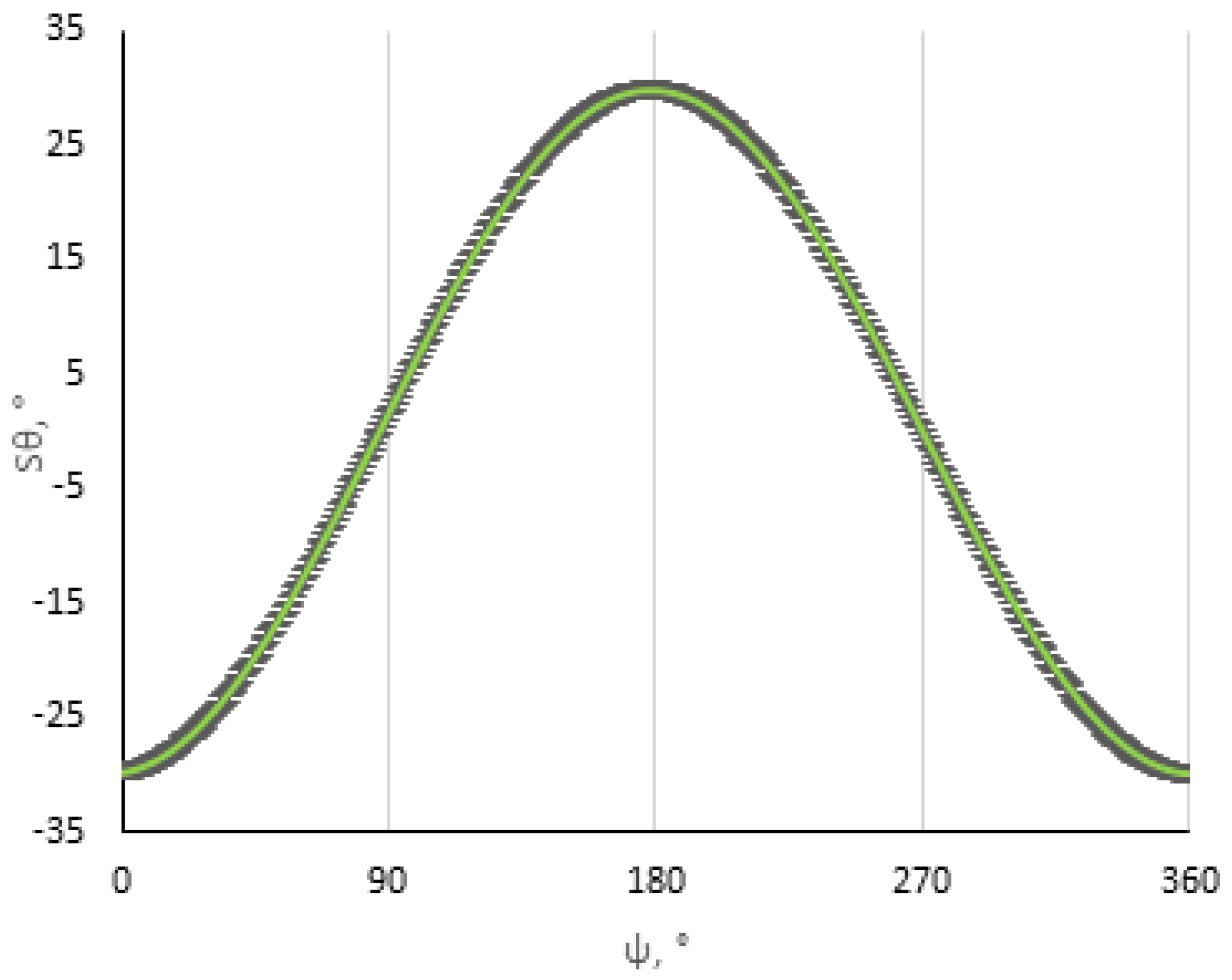
Figure 10 presents the standard uncertainty of composite quantity θ arising due to the measurement of all geometrical quantities of the mechanical control of a fan with a cycloidal rotor for a given amplitude on the testing stand.

To check the history of the real cycloidal function values for a given amplitude, the blade inclination angle θ was measured with the rotor rotated each time by ψ = 1°. A purpose-made angle scale was used with a pitch of 0.5°. The obtained results were then subjected to trigonometric approximation using the sum of sines. The model goodness-of-fit was found at the level of R² = 0.99. The uncertainty of the measurements and standard uncertainties S_xd, S_xe and S_x are listed in

Table 3. Uncertainty of angle θ measurements on the laboratory stand.

Measured Quantities x	Calibration Uncertainty Δdx	Experimenter Uncertainty Δex	Standard Calibration Uncertainty Sxd	Standard Experimenter Uncertainty Sxe	Standard Uncertainty Sx
θ	0.5°	1°	0.29°	0.58°	0.65°

.

Figure 11 presents the curve illustrating the actual cycloidal function values together with the uncertainty due to the measurement of angle θ.

In this case, for each position of the blade, the measurement was performed only once and with the same measuring instrument. For this reason, the uncertainty value does not change with the function values.

Figure 12 presents a comparison between the model and the actual function together with standard uncertainties for the two functions. Good agreement between the functions can be observed—the uncertainty areas overlap, which means that the mechanical control structure and the control settings for a given amplitude of θ₀ are made correctly.

5. Analysis of the Example Case Results

Measurements were performed of a fan with a cycloidal rotor equipped with CLARK Y profile blades, operating with the amplitude of θ₀ ≈ 60° at the rotational speed of 1000 rpm. Figure 13 presents a view of the fan with a cycloidal rotor placed in a rectangular channel with marked measuring meshes. The measurements were carried out using the LDA (Laser Doppler Anemometry) technique [30,31,32].

Figure 13b presents the CRF measuring stand with two measuring meshes: the inlet and the outlet mesh [32]. The inlet measuring mesh (red vertical line in Figure 13b) was generally a straight line made of 23 measuring points. It is distanced from the rotor center by −2R, i.e., by the rotor doubled radius (14 cm). The outlet mesh is located at a distance of 2R from the rotor center and has a rectangular shape. The mesh total dimensions are 28 × 23 cm. Due to the mesh shape and size, both vertical and horizontal velocity profiles could be obtained, but in this paper, only the results of the vertical velocity profiles are presented: −2R (inlet) and 2R, 4R and 6R (outlet). In the beginning, due to the similarity of the curves and relatively small angular differences between individual functions, it was decided to implement the theoretical function into the numerical model created in Ansys CFX. However, due to the limitations of the CFX computations related to the analysis of objects moving towards each other and changing the angle of rotation along with the rotation of the entire rotor, it was necessary to write a script in the Ansys CEL environment that fully enabled the rotor to work based on the cycloidal function. The program rotated the large, round domain with a shaft (Figure 14—2 Inner domain with shaft) in which there were four blades. In each moment of domain rotation, the blade pitch angle θ varied based on the given cycloid function. The geometry of the numerical model used is shown in Figure 14.

The numerical model consisted of three elements: shortened rectangular duct, inner domain with shaft and blades domains. The dimension of the duct geometry used in the CFD was 250 × 25 cm. Inside the channel there is an inner rotor domain with a shaft. The domain diameter was 23 cm and 1.5 cm for the shaft. The blade domains visible in Figure 14 were characterized by a diameter of 8 cm

It was decided to shorten the channel inlet to speed up the calculations. Numerical calculations were performed, and no significant difference was obtained due to the shortening of the canal. In the numerical model, friction was turned off for the tunnel walls, blades and shaft. On the inlet pressure and temperature were set, and on the outlet the “opening” condition was set.

A 2D analysis of four meshes of density from 50 to 400 k elements and the influence of the time step amounting to 360, 720 and 1440 (rotor rotation performed every 1; 0.5 and 0.25°) was made. The best results were obtained for the numerical model consisting of 200 k elements and rotating according to the time step of 720 (rotor rotation is performed every 0.5°).

SST was selected as the turbulence model. It is popular for this type of computation as it combines the advantages of the k-ε and the k-ω models [36]. Based on the described numerical model, two variants of the CLARK Y rotor were created: one working according to the theoretical cycloid function, the other based on the actual cycloid function. The analysis was performed for the amplitude θ₀ = 60° and the rotor speed of 1000 rpm. The results were compared with the experimental data (Figure 14), considering the standard deviation determined by the LDA. The flow velocity C was divided into component velocities Cx and Cy according to the diagram shown in Figure 13.

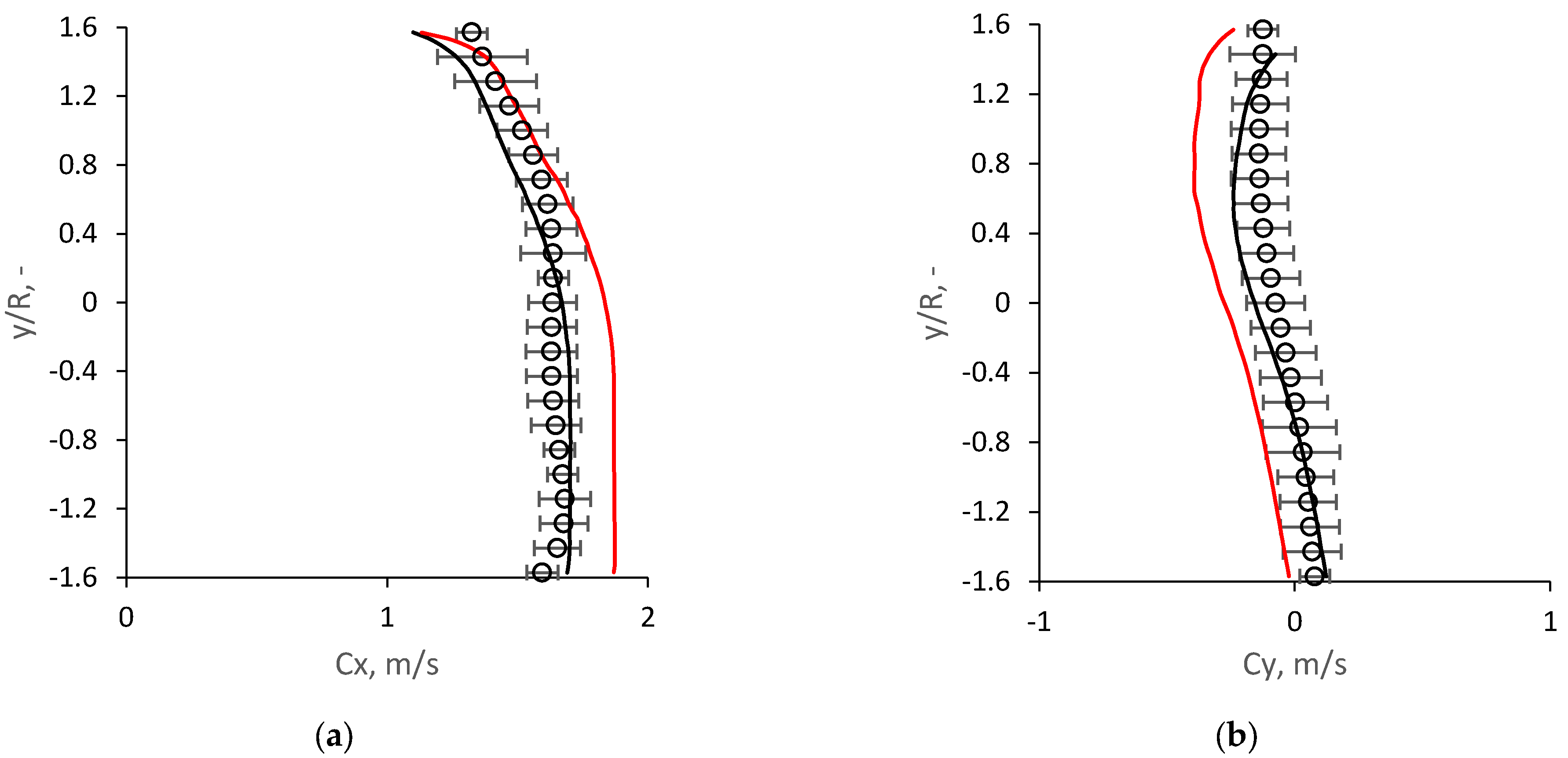
Figure 15 presents the comparison of velocity profiles for individual vertical measuring planes obtained for two CFD variants and the experiment with standard deviations. The X-axis shows the Cx or Cy velocity component, while the Y-axis shows the channel height related to the rotor radius R. The first variant of the rotor was based on changes in the inclination angle according to the theoretical cycloidal function, whereas the second was according to the actual function. Although the angular differences between functions these two functions are relatively small (cf. Figure 2), significant differences can be noticed in the shape of the profiles for the two variants. On the inlet plane (Figure 15a,b), a similar shape of the velocity profiles can be observed for both variants of the rotor operation. Observing the Cx velocity profile, it can be noticed that the rotor draws the stream practically across the entire width of the channel, with a slight difference in the upper part of the channel.

The slight reduction in speed in this part is due to the shape of the Cy speed profile. For both variants, the flow slightly bends towards the bottom of the rotor. This behavior may be caused by the blades breaking off when drawing the stream into the impeller. In the case of the second variant, the numerical model satisfactorily coincides with the experiment, while the results of the first variant slightly differ from it.

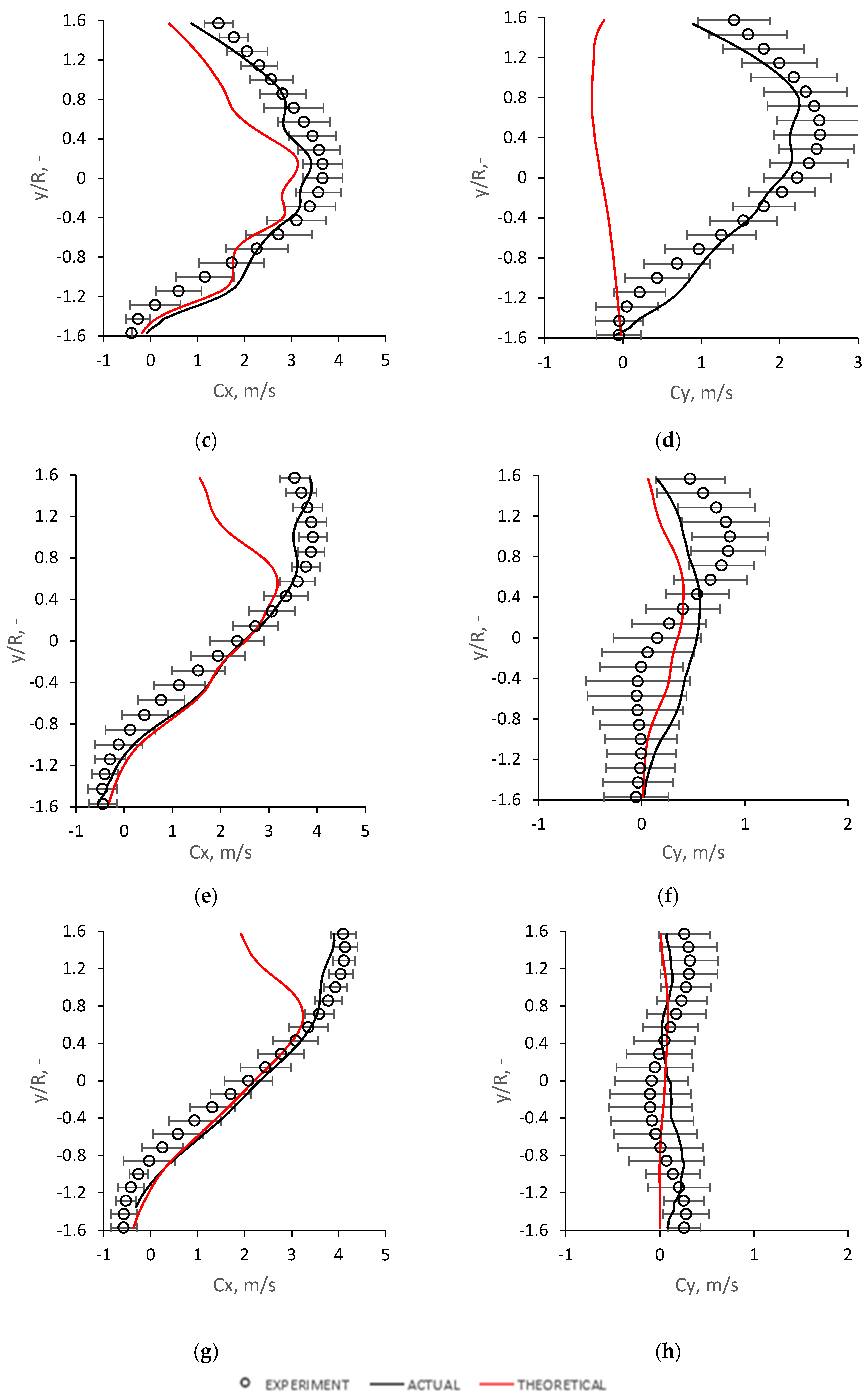
Directly at the rotor outlet (plane 2R), a significant change can be seen for both velocity components (Figure 15c,d) for CFD. Observing the Cx velocity profile, it can be noticed that the flow moves practically in the center of the channel, which is indicated by the positions of the flow front. For the second variant, a satisfactory compliance of the numerical calculations of the fan performing the current function was obtained, which is indicated by the correlation between the CFD results and the experiment values. Among all the analyzed measurement planes, the values of the standard deviation determined by the LDA are the highest in this plane. This means that the flow is the most irregular in this plane, which is caused by the displacement nature of the machine and the reverse action of the rotor. There are areas of turbulence in the lower part of the channel, which is accounted for by the presence of negative velocities.

In the case of the Cy component, the speed profile of the rotor operating based on the theoretical function differs significantly from the actual flow profile. Only the application of the actual function allows us to obtain a good compliance of the CFD with the experiment. The flow shows a similar tendency as for the Cx component, which will cause the stream to move towards the upper wall of the tunnel. The occurrence of such high velocities in this element is dictated by the operation of the rotor, which projects the flow at a certain angle.

By observing the Cx (Figure 15e,f) component, the flow front has moved more in this direction, and therefore the turbulence area in the lower part of the channel has increased. There is a difference in the upper part of the channel between the two analyzed rotor variants in CFD. Looking at the Cy component, it can be noticed a significant speed reduction compared to the 2R plane. The appearance of the characteristic convexity of the velocity profile in the upper part of the channel in the case of the experiment may suggest further movement of the flow front towards the wall.

Similar behaviors of Cx and Cy profiles can be observed for the last measurement plane (Figure 15g,h). The only noticeable difference in the Cx component is that the flow front is slightly directed towards the upper wall, and the turbulence area is enlarged. The velocity profile and its values for the Cy component suggest that further changes in the flow direction will be small. Comparing the models of both presented cycloidal functions, it can be noticed despite theoretically small angular differences. The flow generated by the two impellers is different. This means that relatively small differences arising during the performance of the relevant elements of cycloidal regulation, or their regulation, may contribute to a change in the CRF flow parameters. In the case of prototyping, this risk can be reduced by making correspondingly larger prototypes [18], which, however, is associated with higher production costs.

For the variant with the current cycloidal function, a satisfactory agreement was obtained with the experimental data. Attention should be paid to the significant values of standard deviations, which indicate irregularities in the flow caused by the displacement of the cycloidal rotor.

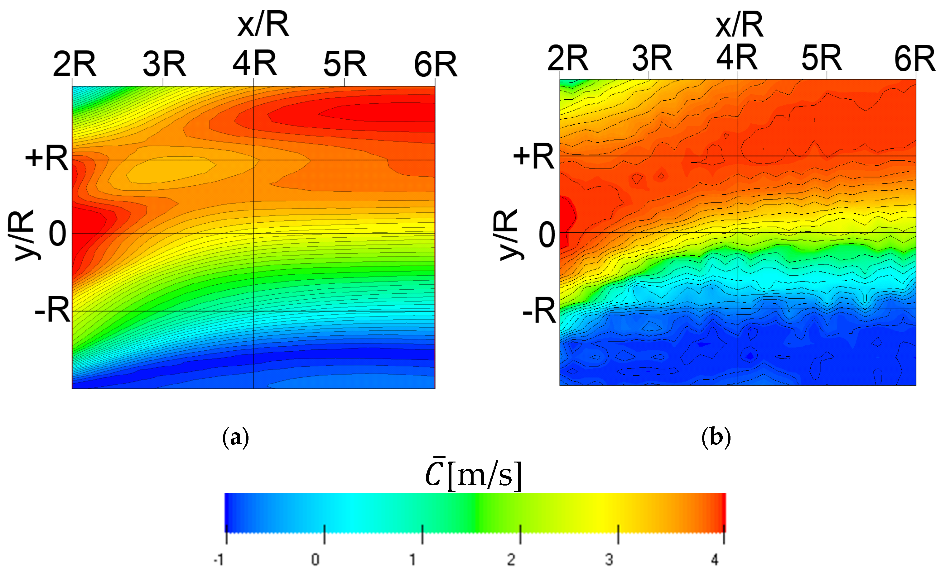
Inhouse “Mesh” software programmed in Python was used to obtain contour maps from LDA measurement data. Based on the outlet grid shown in Figure 13, the LDA flow fields for the absolute velocity of the flow, C, were compared to the CFDs.

Figure 16 shows the velocity fields for CFD and LDA. It can be considered that there was a satisfactory agreement between the experiment and the CFD. The actual flow has a slightly higher speed in the main part. A larger area of reverse flow is visible at the bottom of the channel. The lower level of turbulence in the CFD model is due to the SST model used. For both velocity contours, the area of the stream slowing down (between 2R and 4R) is visible as a result of a change in its direction.

6. Summary and Conclusions

The influence of the values of geometrical parameters on the function curve is shown based on the actual cycloidal function performed by the fan with a cycloidal rotor. The used values correspond to the structure. Based on the analysis results, the following conclusions can be drawn:

• A sensitivity analysis was conducted of the model cycloidal function, varying parameters L, d and e by ±1 mm and ε—by ±10°. Each change in the parameter by 1 mm causes angular changes in the function by about 2°, which may seem insignificant in relation to amplitude θ₀. However, in the case of the rotor operation with its smaller value, it may have a great impact on the real cycloidal function.
• The problem of the cycloidal function sensitivity can be solved by designing bigger CRFs, where the impact of various structural imperfections of the rotor or the mechanical control on the proper cycloidal function will be much smaller.
• An analysis of standard uncertainty was conducted for individual geometrical parameters L, d, e and ε and also for θ using the propagation rule. The uncertainty of θ was affected most by changes in e and L, whereas the impact of d and ε was the smallest.
• Standard uncertainty was determined for θ, taking account of standard uncertainties for all the geometrical quantities e, L, d and ε. The results indicate variability in the range of 1.4–2.4°.
• The final step of the analysis was to determine standard uncertainty for the measurements of θ during the construction of the actual function. A comparison was made between the model and the actual function, together with uncertainties presented for them, and a good agreement between the two functions was obtained. The uncertainty areas overlap, which means that the mechanical control was designed correctly, and its settings during the measurements were selected appropriately.
• Two identical numerical CFD models with different implemented functions were compared with the experiment. The variant with the implemented theoretical function, despite slight differences in the shape of the function curve, gave different results compared to the CRF operating based on the actual cycloidal function. The theoretical model was characterized by a slightly smaller flow rate and the flow tendency to move closer to the middle of the channel, where real values of the flow velocity were higher and where the flow was directed more towards the top of the channel.