Aggregation of Demand-Side Flexibilities: A Comparative Study of Approximation Algorithms

Abstract

Traditional power grids are mainly based on centralized power generation and subsequent distribution. The increasing penetration of distributed renewable energy sources and the growing number of electrical loads is creating difficulties in balancing supply and demand and threatens the secure and efficient operation of power grids. At the same time, households hold an increasing amount of flexibility, which can be exploited by demand-side management to decrease customer cost and support grid operation. Compared to the collection of individual flexibilities, aggregation reduces optimization complexity, protects households’ privacy, and lowers the communication effort. In mathematical terms, each flexibility is modeled by a set of power profiles, and the aggregated flexibility is modeled by the Minkowski sum of individual flexibilities. As the exact Minkowski sum calculation is generally computationally prohibitive, various approximations can be found in the literature. The main contribution of this paper is a comparative evaluation of several approximation algorithms in terms of novel quality criteria, computational complexity, and communication effort using realistic data. Furthermore, we investigate the dependence of selected comparison criteria on the time horizon length and on the number of households. Our results indicate that none of the algorithms perform satisfactorily in all categories. Hence, we provide guidelines on the application-dependent algorithm choice. Moreover, we demonstrate a major drawback of some inner approximations, namely that they may lead to situations in which not using the flexibility is impossible, which may be suboptimal in certain situations.

1. Introduction

Modern power grids must integrate a growing number of decentralized, small-scale renewable energy sources. In addition, climate change, decreasing fossil reserves, and tax regulations are leading to an increase in electrical demand, e.g., through the switch in private mobility from conventional to electric vehicles. As a result, increasing intermittent generation and demand lead to difficulties in balancing supply and demand, which in turn threaten the secure operation of power grids. Many electrical devices such as air conditioners, heat pumps, water heaters and batteries provide operation flexibility and hence there is a prospect for minimizing the operation cost or for providing ancillary services. However, the coordinated control of a large number of flexible devices is challenging due to the computational complexity, communication effort and privacy issues. Therefore, to address these issues, the concept of an aggregator is introduced in the literature.

An aggregator is an entity that can assess and control individual demand-side flexibilities, cf. [1,2] for detailed information. The aggregator sells system services to a utility and thereby acts as an intermediary between contracted consumers and the utility. To this end, the aggregator calculates the aggregated flexibility, which is subsequently communicated to the utility to perform optimization tasks. The utility sends back a requested power profile which has to be disaggregated and distributed by the aggregator to the consumers’ devices. This approach reduces the utility’s optimization complexity and communication effort as only aggregated variables and constraints are concerned. In addition, the privacy of consumers is preserved if only the aggregator handles individual consumer data and is allowed to control consumer devices. Therefore, a key challenge is the mathematical modeling and tractable computation of the aggregated flexibility.

We consider a setting in which an aggregator controls household flexibilities provided by batteries serving as electrical energy storages. However, our setting is extendable, for example, to thermostatically controlled loads (TCLs) which can be described by general battery models [3,4]. In mathematical terms, the flexibility of a household can be described by the set of all power profiles by which the household’s demand profile can differ from the default demand profile of no flexibility. The aggregated flexibility over all households is then described by the Minkowski sum (M-sum) of individual flexibilities. However, existing algorithms for M-sum calculations are very expensive [5]. Consequently, different approximations of the aggregated flexibility have been proposed in the literature. These methods range from one step ahead to multi-step ahead and from bottom–up to top–down approaches. Top–down approaches attempt to directly capture the aggregated flexibility, for example, by using probability distributions or Markov transition matrices [6,7,8,9]. In this paper, we consider bottom–up multi-step ahead approaches which start from individual flexibility sets. Approximations are further divided into inner and outer approximations. Outer approximations typically overestimate the aggregated flexibility, while inner approximations typically do not capture the full aggregated flexibility. Consequently, the main disadvantage of outer approximations is that not all set elements can be disaggregated among the individual flexibilities. For inner approximations, on the other side, some flexibility is generally lost.

We very briefly review some typical approximation approaches. A more detailed description of the approximations evaluated in this paper is given in Section 3. Outer approximations for linear, second-order cone, and semi-definite constraints were developed in [4,10]. The authors determined the accuracy of their approximation by comparing the volume of the approximation to the volume of the exact aggregated flexibility, where the volumes were estimated using a Monte Carlo procedure. In addition, they compared the approximation for linear constraints with the approximation derived in [11] and reported that their approximation is more accurate by a factor of 1.5–2. He Hao et al. [11,12] developed approximations based on a generalized battery model, in which the battery parameters are analytically derived to obtain inner and outer approximations. The authors in [13,14] used zonotopes, which are centrally symmetric polytopes, as inner approximations to the individual flexibility polytopes. The benefit of this approach is that the M-sum of zonotopes is computationally efficient. Nazir et al. [15] introduced an inner approximation whereby each individual polytope is decomposed into a collection of cuboid-homothets. Homothets are scaled and translated sets of a prototype set, e.g., a cuboid, and also have the advantage that their M-sum can be efficiently computed. The authors tested their approximation by relating the estimated volume of the approximation to the estimated volume of the exact aggregated flexibility. They reported that their approximation covered 44% of the exact M-sum for stage 0 and 74% for stage 1. Zhao et al. [3] developed inner and outer approximations based on homothets where the difference to the latter approach is two-fold: first, the authors used more general prototype sets than cuboids; and second, only one homothet per polytope is fitted. The authors tested their approximation against the approximations developed in references [12,16] in a setting with 1000 heterogeneous TCLs, and reported a better coverage of exact flexibility. The authors in [17,18] developed inner approximations based on ellipsoidal projection. In this approach, the M-sum is first implicitly described in a higher-dimensional space. An ellipsoid with a maximum volume is fitted into this set. Subsequently, the projection of the ellipsoid on the original space represents an inner approximation. Barot [17] reported, based on a volumetric consideration, that the approach of Zhen and Den Hertog [18] provides a superior approximation. Zhao et al. [19] applied a homothet projection method to obtain an inner approximation. Appino et al. [20] first added the individual power and energy constraints which lead to an outer approximation. In a second step, the approximations of the aggregated flexibility are constructed, whereby feasible disaggregation is guaranteed.

Despite the large number of approximation strategies documented in the literature, to the best of the authors’ knowledge, no study exists that benchmarks and compares them. The main contributions of this paper are:

• We evaluate 10 inner and 3 outer M-sum approximations on real, publicly available data with varying battery settings;
• We propose novel practice-oriented criteria to assess the quality of approximations and evaluate them on several algorithms;
• We compare the computational complexity and the communication effort associated with the selected algorithms;
• We make the code and the detailed results available in a publicly accessible repository giving future authors a tool to evaluate and compare their approximations.

The remainder of this paper is organized as follows: The system model, the general approximation problem and the data sources are described in Section 2. Section 3 describes the M-sum approximations considered in this paper. Section 4 presents the evaluation framework, i.e., the quality criteria to evaluate the accuracy of the approximations and the simulation settings. Finally, we present and discuss the results in Section 5 and draw conclusions in Section 6.

2. Preliminaries

This section presents the system model, i.e., the mathematical description of the applied setting along with the assumptions made, the approximation problem, and the data used.

2.1. System Model

We consider M quarter-hourly time periods and N households equipped with stationary batteries. Each household $i\in \{1,\dots ,N\}$ has a demand profile $d_i\left(t\right)$ (kW), a power exchange with the grid $g_i\left(t\right)$ (kW) and a battery charge–discharge power $x_i\left(t\right)$ (kW) for time periods $t\in \{1,\dots ,M\}$. Positive values of $x_i\left(t\right)$ and $g_i\left(t\right)$ correspond to charging the battery and drawing electricity from the grid, respectively. Negative values correspond to power flows in the opposite direction. Figure 1 illustrates the system model, the directions of positive power flow, and sketches of two-dimensional household flexibilities.

Each household provides a flexibility, which is communicated to the aggregator. The aggregator calculates an approximation to the M-sum of these flexibilities, which is sent to the utility to perform optimization tasks. Note that we limit our considerations to the flexibility in the active power, so the flexibility provided by the reactive part is not considered. The power balance in each household i can be written as

$$g_i\left(t\right)=x_i\left(t\right)+d_i\left(t\right)\forall t\in \{1,\dots ,M\}$$

(1)

Each household battery i is subject to the following power and energy constraints $\forall t\in \{1,\dots ,M\}$:

$$\begin{array}{cc}\hfill x_{\min ,i}& \le x_i\left(t\right)\le x_{\max ,i}\hfill \end{array}$$

(2)

$$\begin{array}{cc}\hfill S_i\left(t\right)& =S_i(t-1)+x_i\left(t\right)\Delta t\hfill \end{array}$$

(3)

$$\begin{array}{cc}\hfill S_i\left(0\right)& =S_{0,i}\hfill \end{array}$$

(4)

$$\begin{array}{cc}\hfill 0& \le S_i\left(t\right)\le S_{\max ,i}\hfill \end{array}$$

(5)

$$\begin{array}{cc}\hfill S_{\mathrm{end},i}& \le S_i\left(M\right)\le S_{\max ,i},\hfill \end{array}$$

(6)

where $x_{\max ,i}$ and $x_{\min ,i}$ represent the upper and lower power limits (kW), respectively, $S_i\left(t\right)$ the battery energy (kWh) at time t, $S_{\max ,i}$ its capacity (kWh), $S_{0,i}$ its initial energy (kWh), and $S_{\mathrm{end},i}$ its minimum final energy (kWh). Constraints (3)–(6) are equivalently rewritten as

$$\begin{array}{cc}\hfill & 0\le S_{0,i}+\sum _{t=1}^J{x}_i\left(t\right)\Delta t\le S_{\max ,i}\forall J\in \{1,\dots ,M-1\}\hfill \end{array}$$

(7)

$$\begin{array}{cc}\hfill & S_{\mathrm{end},i}\le S_{0,i}+\sum _{t=1}^M{x}_i\left(t\right)\Delta t\le S_{\max ,i},\hfill \end{array}$$

(8)

such that the flexibility of each battery is described by the polytope of vectors $x_i\in {\mathbb{R}}^M$ fulfilling Equations (2), (7) and (8). In matrix notation, the constraints are given by (9)

$$\left(\begin{array}{c}-I\\ I\\ \Gamma \\ -\Gamma \end{array}\right)x_i\le \left(\begin{array}{c}-x_{\min ,i}{\mathbf{1}}_M\\ x_{\max ,i}{\mathbf{1}}_M\\ \frac{S_{\max ,i}-S_{0,i}}{\Delta t}{\mathbf{1}}_M\\ \frac{S_{0,i}}{\Delta t}{\mathbf{1}}_{M-1}\\ \frac{S_{0,i}-S_{\mathrm{end},i}}{\Delta t}\end{array}\right),$$

(9)

where I is the $M\times M$ identity matrix, $\Gamma$ is an $M\times M$ lower triangular matrix with values of one, and ${\mathbf{1}}_n$ is the n-vector of ones, cf. [21]. We identify the left matrix in (9) as A and the right-hand side vector as $b_i$. Hence, the flexibility of household i can be succinctly written as

$$\mathcal{P}(A,b_i)=\{x_i\in {\mathbb{R}}^M|A{x}_i\le b_i\}$$

(10)

Note that the matrix A is the same for all households. Finally, the exact aggregated flexibility of N households is expressed by the M-sum of individual flexibilities as follows.

$${\mathcal{X}}_{\mathrm{exact}}={\oplus }_{i=1}^N\mathcal{P}(A,b_i)=\left\{x\in {\mathbb{R}}^M|x=\sum _{i=1}^N{x}_i,x_i\in \mathcal{P}(A,b_i)\right\}$$

(11)

2.2. Approximation Problem

The set ${\mathcal{X}}_{\mathrm{exact}}$ represents the aggregate grid operation flexibility on the demand side. Its computation is, however, in general intractable. Therefore, it is important to find accurate and efficiently computable approximations. An approximation set ${\mathcal{X}}_{\mathrm{approx}}$ is called outer approximation (OA) if ${\mathcal{X}}_{\mathrm{approx}}\supseteq {\mathcal{X}}_{\mathrm{exact}}$ and inner approximation (IA) if ${\mathcal{X}}_{\mathrm{approx}}\subseteq {\mathcal{X}}_{\mathrm{exact}}$, cf. Figure 2. Different measures for approximation accuracy can be conceived. In Section 4, we define quality criteria which are relevant for grid operators and utilities who optimize some objective function over ${\mathcal{X}}_{\mathrm{approx}}$.

2.3. Data

We used publicly available household demand data consisting of the half-hourly energy consumption of residential consumers from July 2009 to December 2010 in Ireland [22]. The publicly available hourly day-ahead prices for the Germany–Austria–Luxembourg region from 2016 were used as energy prices [23]. Both data sets were resampled to quarter-hourly data and time-synchronized with the publicly available code of [24]. The battery parameters were uniformly sampled from the following intervals: $S_{\max ,i}\in [10.5,13.5]$ (kWh), $S_{0,i}\in [0,10.5]$ (kWh), $x_{\max ,i}\in [4,6]$ (kW), and $x_{\min ,i}\in [-6,-4]$ (kW) ∀ i $\in \{1,\dots ,N\}$. The minimal final battery energy was set to half of its initial value: $S_{\mathrm{end},i}=S_{0,i}/2$ ∀ i $\in \{1,\dots ,N\}$.

3. Overview of Approximation Strategies

In this section, we present the implemented inner and outer approximations in a unified notation and adapted to our system model, such that expressions for computational complexity and communication effort can be derived on a common ground. The approximations are presented in a mathematically coherent order. First, the summation-based approximations are presented, followed by the zonotope- and homothet-based approximations, and finally the projection based approximations. More detailed descriptions of the algorithms can be found in the literature references.

3.1. Outer Approximation by Right-Hand Sides Summation

This outer approximation was developed by Barot and Taylor [4,17]. Let N households with feasible regions $\mathcal{P}(A,b_i)$ be given, then an outer approximation to the M-sum is described by the set:

$${\mathcal{X}}_{\mathrm{approx}}=\left\{x\in {\mathbb{R}}^M|Ax\le \sum _{i=1}^N{b}_i\right\}.$$

(12)

For M time periods, $4M(N-1)$ summations are needed. Note that $4M$ is the amount of rows in A for the setting described in Section 2.1. The communication effort consists of sending the $4M\times M$ matrix A and the $4M$-vector ${\sum }_{i=1}^N{b}_i$ of the right-hand sides (RHSs) summation to the utility.

3.2. Outer Approximation by Right-Hand Sides Summation with Preconditioning

This approximation of Barot and Taylor [4,17] is an extension of the previous approximation, where each $b_i$ is maximally shrunk before summation. The flexibility, which is given by the feasible region of the constraints, is not changed by this preconditioning (PC). The hyperplanes describing these constraints are shifted such that each one supports the feasible region $\mathcal{P}(A,b_i)$. In detail, let $a_j$ be the jth row of A, then the following linear program is solved to recompute the jth entry of $b_i$:

$$\begin{array}{cc}\hfill {\tilde{b}}_i\left(j\right)=\underset{x}{max}& a_j^{\top }x\hfill \\ \hfill \mathrm{s}.\mathrm{t}.& Ax\le b_i\hfill \end{array}$$

(13)

In total, $4MN$ linear programs with each $4M$ constraints and M variables have to be solved. The outer approximation to the M-sum is described by the set:

$${\mathcal{X}}_{\mathrm{approx}}=\left\{x\in {\mathbb{R}}^M|Ax\le \sum _{i=1}^N{\tilde{b}}_i\right\}.$$

(14)

The communication effort again consists of transmitting the $4M\times M$ matrix A and the $4M$-vector ${\sum }_{i=1}^N{\tilde{b}}_i$ to the utility.

3.3. Inner Approximation with Zonotopes

Müller et al. [13,14] used zonotopes to obtain an inner approximation to the M-sum. Zonotopes are centrally symmetric polytopes described by

$${\mathcal{Z}}_i(G,{\nu }_i,{\overline{\lambda }}_i)=\left\{x\in {\mathbb{R}}^M|x={\nu }_i+G\lambda ,-{\overline{\lambda }}_i\le \lambda \le {\overline{\lambda }}_i\right\},$$

(15)

where G is a matrix with normalized column vectors serving as generating directions; $\lambda$ is a vector of scaling factors; and ${\nu }_i$ is the zonotope center. Following the approach of [13], we choose the M unit vectors and additional $M-1$ vectors of the form

$${(0,\dots ,-\frac{1}{\sqrt{2}},\frac{1}{\sqrt{2}},\dots ,0)}^{\top }$$

as generating directions.

To compute the matrix C of the zonotope half-space representation $\{x\in {\mathbb{R}}^M|Cx\le u_i\}$, Müller et al. [14] showed that at most $M^2+M$ normals, i.e., rows in C, have to be computed. Subsequently, the offsets $u_i$ are calculated by shifting the zonotope hyperplanes such that each one supports the given polytope $\mathcal{P}(A,b_i)$. This step is analogous to problem (13) and requires the solution of at most $M^2+M$ linear programs per household. The final step is to find inner approximation zonotopes with respect to a given objective. The constraint that enforces a zonotope to be a subset of a given polytope is given in [14] as

$${\mathcal{Z}}_i(G,{\nu }_i,{\overline{\lambda }}_i)\subseteq \mathcal{P}(A,b_i)\iff A{\nu }_i+\left|AG\right|{\overline{\lambda }}_i\le b_i$$

(16)

where $\left|AG\right|$ is the element-wise absolute value of the matrix $AG$. In [13], the optimal inner zonotopes are found by minimizing the distance between the offsets in a given norm:

$$\begin{array}{cc}\hfill \underset{{\nu }_i,{\overline{\lambda }}_i}{min}& {\parallel u_i-{\delta }_Z({\nu }_i,{\overline{\lambda }}_i)\parallel }_l\hfill \\ \hfill \mathrm{s}.\mathrm{t}.& A{\nu }_i+\left|AG\right|{\overline{\lambda }}_i\le b_i\hfill \\ \hfill & {\overline{\lambda }}_i\ge 0\hfill \end{array}$$

(17)

with $l\in \{1,2,\infty \}$. Here, $u_i$ are the previously calculated offsets and:

$${\delta }_Z({\nu }_i,{\overline{\lambda }}_i)=\left(\begin{array}{c}F\\ -F\end{array}\right){\nu }_i+\left(\begin{array}{c}\left|FG\right|\\ \left|FG\right|\end{array}\right){\overline{\lambda }}_i$$

(18)

are the offsets in terms of the center ${\nu }_i$ and the vector of scaling limits ${\overline{\lambda }}_i$, cf. [13,25]. The matrices F and $-F$ contain the zonotope normals.

Müller et al. [14] also proposed a slightly different approximation where problem (19) is solved instead of (17):

$$\begin{array}{cc}\hfill \underset{{\nu }_i,{\overline{\lambda }}_i}{max}& w^{\top }\overline{\lambda }\hfill \\ \hfill \mathrm{s}.\mathrm{t}.& A{\nu }_i+\left|AG\right|{\overline{\lambda }}_i\le b_i\hfill \\ \hfill & {\overline{\lambda }}_i\ge 0\hfill \end{array}$$

(19)

with $w=\frac{2}{M^2+M}{\tilde{u}}_i^{\top }\left|CG\right|$, where ${\tilde{u}}_i$ is the element-wise reciprocal of $u_i$. Finally, the M-sum of these optimal inner zonotopes can be efficiently calculated by summing up the ${\nu }_i$ and ${\overline{\lambda }}_i$ to obtain an aggregate inner approximation:

$${\mathcal{X}}_{\mathrm{approx}}={\oplus }_{i=1}^N{\mathcal{Z}}_i(G,{\nu }_i,{\overline{\lambda }}_i)=\mathcal{Z}\left(G,\sum _{i=1}^N{\nu }_i,\sum _{i=1}^N{\overline{\lambda }}_i\right),$$

(20)

A maximum of $(M^2+M)N$ linear programs with $4M$ constraints and M variables must be solved. In addition, N linear programs with $2M^2+8M-1$ constraints and $M^2+4M-1$ variables for $l_1$ norm, N linear programs with $2M^2+8M-1$ constraints and $3M$ variables for $l_{\infty }$ norm, N convex programs with $6M-1$ constraints and $3M-1$ variables for $l_2$ norm and N linear programs with $6M-1$ constraints and $3M-1$ variables for problem (19) are solved. The communication effort consists of transmitting the $M\times 2M-1$ matrix of generators G, the sum of M dimensional centers ${\nu }_i$ and the sum of $2M-1$-vectors ${\overline{\lambda }}_i$ to the utility.

3.4. Inner Approximation with Cuboid Homothets

Nazir et al. [15] used unions of homothets to compute an inner approximation to the aggregate flexibility. Given a compact convex set ${\mathcal{P}}_0$, a homothet of ${\mathcal{P}}_0$ is defined as the set:

$${\beta }_i{\mathcal{P}}_0+t_i:=\{x\in {\mathbb{R}}^M|x={\beta }_i\zeta +t_i,\zeta \in {\mathcal{P}}_0\}$$

(21)

with ${\beta }_i>0$. The key idea is to decompose each polytope $\mathcal{P}(A,b_i)$ into a collection of homothets. Following [15], the maximum volume cuboid that fits into, for example, the first polytope $\mathcal{P}(A,b_1)$ is taken as the prototype set ${\mathcal{P}}_0$ by solving:

$$\begin{array}{cc}\hfill \underset{x^{+},x^{-}}{max}& \prod _{k=1}^M{x}_k^{+}-x_k^{-}\hfill \\ \hfill \mathrm{s}.\mathrm{t}.& A^{+}{x}^{+}-A^{-}{x}^{-}\le b_1\hfill \\ \hfill & x_k^{-}\le x_k^{+},\mathrm{for}k=1,\dots ,M,\hfill \end{array}$$

(22)

where $A_{ij}^{+}=max(0,A_{ij})$ and $A_{ij}^{-}=max(0,-A_{ij})$, cf. [26]. The objective in (22) can be equivalently replaced by ${\sum }_{k=1}^{M}log(x_k^{+}-x_k^{-})$, which leads to a convex problem that can be solved by CVXPY [27]. Subsequently, the edge distances ${\delta }_k^0=(x_k^{+}-x_k^{-})$ for $k\in \{1,2,\dots ,M\}$ and the distance ratios ${\rho }_{1,k}^0={\delta }_1^0/{\delta }_k^0$ for $k\in \{2,\dots ,M\}$ are calculated. The following optimization problems find the maximum volume homothets of ${\mathcal{P}}_0$ in all $\mathcal{P}(A,b_i)$ for $i\in \{1,\dots ,N\}$:

$$\begin{array}{cc}\hfill \underset{x^{+},x^{-}}{max}& \prod _{k=1}^M{x}_k^{+}-x_k^{-}\hfill \\ \hfill \mathrm{s}.\mathrm{t}.& A^{+}{x}^{+}-A^{-}{x}^{-}\le b_i\hfill \\ \hfill & x_k^{-}\le x_k^{+},\mathrm{for}k=1,\dots ,M\hfill \\ \hfill & (x_1^{+}-x_1^{-})={\rho }_{1,k}^0(x_k^{+}-x_k^{-}),\mathrm{for}k=2,\dots ,M\hfill \end{array}$$

(23)

Note that the last constraint enforces the solution to be a homothet of ${\mathcal{P}}_0$.

This procedure can be applied in several stages to cover more flexibility: in stage zero, a maximum volume homothet of ${\mathcal{P}}_0$ is fitted into each $\mathcal{P}(A,b_i)$. In stage one, maximum volume homothets of ${\mathcal{P}}_0$ are fitted into regions not covered by the stage zero solution. This is performed by extending matrix A and vector $b_i$ by a row of the half-space inequalities of the stage zero solution multiplied by −1. The procedure is shown for stages zero and one in Figure 3.

Each stage s requires the solution of at most ${\left(2M\right)}^s$ optimization problems leading to a total of at most ${\sum }_{i=0}^s{\left(2M\right)}^i=\frac{{\left(2M\right)}^{s+1}-1}{\left(2M\right)-1}$ convex problems per household.

Finally, the distributive property of the M-sum is used to obtain an inner approximation to the aggregated flexibility, i.e., instead of first forming the union and then the M-sum, the M-sum is performed first and then the union. Nazir et al. [15] proposed to only use corresponding combinations for axis-aligned cuboids, e.g., the kth cuboid of the sth stage in $\mathcal{P}(A,b_i)$ is added to the kth cuboid of the sth stage in $\mathcal{P}(A,b_j)$. The M-sum of homothets is given by

$${\oplus }_{i=1}^N({\beta }_i{\mathcal{P}}_0+t_i)=\sum _{i=1}^N{\beta }_i{\mathcal{P}}_0+\sum _{i=1}^N{t}_i.$$

(24)

When using cuboids, this can be simplified to the summation of the right-hand vectors in the half-space representation.

The total computational effort consists of solving $N{\left(2M\right)}^0$ convex problems with $(6M-1)$ constraints and $2M$ variables for stage 0, $N{\left(2M\right)}^1$ convex problems with $(6M-1+1)$ constraints and $2M$ variables for stage 1, up to $N{\left(2M\right)}^s$ convex problems with $(6M-1+s)$ constraints and $2M$ variables for stage s. In addition, one convex problem with $5M$ constraints and $2M$ variables has to be solved. The communication effort consists of sending the $2M\times M$ matrix ${(I,-I)}^{\top }$, the $2M$-vector ${(x^{+},-x^{-})}^{\top }$ as solutions to problem (22) and a maximum of $\frac{{\left(2M\right)}^{s+1}-1}{2M-1}$ scaling factors ${\beta }_j$ and M dimensional offsets $t_j$ to the utility.

3.5. Inner Approximation with Battery Homothets

Zhao et al. [3] used the battery model (9) as the prototype set ${\mathcal{P}}_0$ to obtain inner homothet approximations. They used the average individual battery parameters as prototype battery parameters which we denote with $b_p$, i.e., ${\mathcal{P}}_0=\{x\in {\mathbb{R}}^M|Ax\le b_p\}$. To find the maximum volume homothet of ${\mathcal{P}}_0$ in $\mathcal{P}(A,b_i)$ one solves:

$$\begin{array}{cc}\hfill \underset{{\beta }_i,t_i}{max}& {\beta }_i\hfill \\ \hfill \mathrm{s}.\mathrm{t}.& {\beta }_i{\mathcal{P}}_0+t_i\subset \mathcal{P}(A,b_i)\hfill \\ \hfill & {\beta }_i>0.\hfill \end{array}$$

(25)

In [3], it is shown that the solution to this problem is given by ${\beta }_i^{★}=\frac{1}{s_i^{★}}$ and $t_i^{★}=-\frac{r_i^{★}}{s_i^{★}}$ if $(s_i^{★},r_i^{★},G^{★})$ is the solution of:

$$\begin{array}{cc}\hfill \underset{s_i,G,r_i}{min}& s_i\hfill \\ \hfill \mathrm{s}.\mathrm{t}.& GA=A\hfill \\ \hfill & G{b}_p\le s_i{b}_i+A{r}_i\hfill \\ \hfill & s_i>0,G\ge 0,\hfill \end{array}$$

(26)

where $G\ge 0$ means element-wise inequality. Once the inner approximation for all $\mathcal{P}(A,b_i)$ is obtained, the M-sum of these homothet approximations can be calculated using Equation (24). The overall computation effort is given by solving N linear programs with $20M^2+4M+1$ constraints and $16M^2+M+1$ variables. The communication effort consists of transmitting the $4M\times M$ matrix A, the $4M$-vector $b_p$, the sum of the scaling factors ${\beta }_i$, and M dimensional offsets $t_i$ to the utility.

3.6. Outer Approximation with Battery Homothets

Zhao et al. [3] also developed a homothet outer approximation using the same prototype set ${\mathcal{P}}_0=\{x\in {\mathbb{R}}^M|Ax\le b_p\}$. To obtain the outer approximation to $\mathcal{P}(A,b_i)$, one has to solve:

$$\begin{array}{cc}\hfill \underset{{\beta }_i,t_i}{min}& {\beta }_i\hfill \\ \hfill \mathrm{s}.\mathrm{t}.& {\beta }_i{\mathcal{P}}_0+t_i\supset \mathcal{P}(A,b_i)\hfill \\ \hfill & {\beta }_i>0\hfill \end{array}$$

(27)

which can be reformulated as

$$\begin{array}{cc}\hfill \underset{{\beta }_i,G,t_i}{min}& {\beta }_i\hfill \\ \hfill \mathrm{s}.\mathrm{t}.& GA=A\hfill \\ \hfill & G{b}_i\le {\beta }_i{b}_p+A{t}_i\hfill \\ \hfill & {\beta }_i>0,G\ge 0\hfill \end{array}$$

(28)

The M-sum of the homothet approximations is again calculated by (24). Similarly to the previous approximation, the overall computation effort is given by N linear programs with $20M^2+4M+1$ constraints and $16M^2+M+1$ variables. The $4M\times M$ matrix A, the $4M$-vector $b_p$, the sum of the scaling factors ${\beta }_i$, and M dimensional offsets $t_i$ must be transmitted to the utility.

3.7. Inner Approximation by Ellipsoid Projection

Barot [17] assumes that N households with feasible regions $\mathcal{P}(A,b_i)$ are given. The M-sum can be implicitly written as

$$\left\{z\in {\mathbb{R}}^M|\left(\begin{array}{cccccc}\hfill A& \hfill -A& \hfill -A& \hfill \dots & \hfill -A& \hfill -A\\ \hfill 0& \hfill A& \hfill 0& \hfill \dots & \hfill 0& \hfill 0\\ \hfill ⋮& \hfill & & \hfill & & \hfill ⋮\\ \hfill 0& \hfill 0& \hfill 0& \hfill \dots & \hfill A& \hfill 0\\ \hfill 0& \hfill 0& \hfill 0& \hfill \dots & \hfill 0& \hfill A\end{array}\right)\left(\begin{array}{c}z\\ x_1\\ ⋮\\ x_{N-1}\end{array}\right)\le \left(\begin{array}{c}{b}_N\\ b_1\\ ⋮\\ b_{N-1}\end{array}\right)\right\},$$

(29)

where $z={\sum }_{i=1}^N{x}_i$. We denote the left $4MN\times MN$ matrix as Q and the right vector as p; hence, the feasible region is written as $\mathcal{P}(Q,p)$. The main idea is to fit an ellipsoid with maximum volume in this set. An ellipsoid can be written as the image of the unit ball under an affine transformation as

$$\mathcal{E}=\left\{{Gu+h|\parallel u\parallel }_2\le 1\right\},$$

(30)

where the positive definite matrix G and the center h are partitioned as

$$\begin{array}{cc}\hfill & G=\left(\begin{array}{cc}\hfill G_z& \hfill G_{xz}\\ \hfill G_{xz}^{\top }& \hfill G_x\end{array}\right)\hfill \end{array}$$

(31)

$$\begin{array}{cc}\hfill & h=\left(\begin{array}{c}{h}_z\\ h_x\end{array}\right)\hfill \end{array}$$

(32)

with $x={(x_1,\dots ,x_{N-1})}^{\top }$. The volume of the ellipsoid is proportional to $det\left(G\right)$, hence the problem of finding an ellipsoid with maximum volume in $\mathcal{P}(Q,p)$ can be formulated as follows, cf. [28]:

$$\begin{array}{cc}\hfill \underset{G,h}{max}& log(det(G\left)\right)\hfill \\ \hfill \mathrm{s}.\mathrm{t}.& {\parallel G{q}_i\parallel }_2+q_i^{\top }h\le p_i\mathrm{for}i=1,\dots ,4MN\hfill \\ \hfill & G\succ 0\hfill \end{array}$$

(33)

where $q_i$ is the ith row in Q and the notation $G\succ 0$ denotes a positive definite matrix G. Barot [17] proposes to maximize the determinant of the submatrix $G_z$ associated with the M-sum rather than that of G, leading to the following semi-definite program:

$$\begin{array}{cc}\hfill \underset{G,h}{max}& log(det\left(G_z\right))\hfill \\ \hfill \mathrm{s}.\mathrm{t}.& {\parallel G{q}_i\parallel }_2+q_i^{\top }h\le p_i\mathrm{for}i=1,\dots ,4MN\hfill \\ \hfill & G\succ 0\hfill \end{array}$$

(34)

Solving this problem yields an ellipsoid in the z–x space which is projected back on the z space to derive an inner approximation of the aggregate flexibility. Problem (34) can be solved by CVXPY [27]. The computation effort is given by one semidefinite program with $4MN$ constraints and $M^2{N}^2+MN$ variables. The communication effort consists of transmitting the $M\times M$ matrix $G_z$ and the M dimensional center $h_z$ to the utility.

3.8. Inner Approximation by Ellipsoid Projection with Linear Decision Rule

Zhen and Den Hertog [18] developed an inner approximation based on ellipsoidal projection where the inclusion constraint is only defined in z space:

$$\begin{array}{cc}\hfill \underset{h_z,y,G_z}{max}& log(det\left(G_z\right))\hfill \\ \hfill \mathrm{s}.\mathrm{t}.& \forall u\in {\mathcal{B}}^M\exists y\in {\mathbb{R}}^{M(N-1)}:Q\left(\begin{array}{c}{h}_z+G_{z}u\\ y\end{array}\right)\le p,\hfill \end{array}$$

(35)

where ${\mathcal{B}}^M=\{u\in {\mathbb{R}}^M|{\parallel u\parallel }_2\le 1\}$ is the unit ball of dimension M and $\mathcal{P}(Q,p)$ the implicitly described M-sum with matrix Q and right-hand vector p, cf. (29). This problem can be interpreted as a robust optimization problem, where $h_z$ and $G_z$ are the here and now decision variables and y the wait and see variable. Assuming a linear decision rule (LDR) $y=Vu+w$, the above problem can be reformulated as

$$\begin{array}{cc}\hfill \underset{h_z,w,G_z,V}{max}& log(det\left(G_z\right))\hfill \\ \hfill \mathrm{s}.\mathrm{t}.& {∥{\left(\begin{array}{c}{G}_z\\ V\end{array}\right)}^{\top }{q}_i∥}_2+q_i^{\top }\left(\begin{array}{c}{h}_z\\ w\end{array}\right)\le p_i\mathrm{for}i=1,\dots ,4MN\hfill \\ \hfill & G_z\succ 0\hfill \end{array}$$

(36)

Solving this problem yields an ellipsoid in z space which is an inner approximation of the aggregate flexibility. The overall computation effort is given by a semidefinite problem with $4MN$ constraints and $M^{2}N+MN$ variables. The M dimensional center $h_z$ and the $M\times M$ matrix $G_z$ needs to be transmitted to the utility.

3.9. Inner Approximation by Homothet Projection with Linear Decision Rule

Zhao et al. [19] developed an inner approximation based on homothet-projection. Similar to the previous approach, the implicit M-sum description in (29) is used, where the matrix is denoted as Q and the right vector as p, which allows to write the feasible region as $\mathcal{P}(Q,p)$. The battery model derived in (9) is chosen as the prototype set ${\mathcal{P}}_0=\{x\in {\mathbb{R}}^M|Ax\le b_p\}$ where again the battery parameters are taken as the average of the individual battery parameters. For a fixed vector $u_0\in {\mathbb{R}}^{M(N-1)}$, let ${\tilde{\mathcal{P}}}_0=\{{(x,u_0)}^{\top }\in {\mathbb{R}}^{MN}|Ax\le b_p\}$ denote the corresponding lift of ${\mathcal{P}}_0$ in $MN$ dimensional space. The problem of finding a maximal homothet of ${\tilde{\mathcal{P}}}_0$ in $\mathcal{P}(Q,p)$ is formulated as

$$\begin{array}{cc}\hfill \underset{\beta ,t,u_0}{max}& \beta \hfill \\ \hfill \mathrm{s}.\mathrm{t}.& \beta {\tilde{\mathcal{P}}}_0+\tilde{t}\subset \mathcal{P}(Q,p)\hfill \\ \hfill & \beta >0\hfill \end{array}$$

(37)

where $\tilde{t}={(t,0)}^{\top }$ is the lift of t in $MN$ dimensional space by setting the additional dimensions to zero. This problem is transformed by the authors to the following linear program:

$$\begin{array}{cc}\hfill \underset{s,G,r,u_0}{min}& s\hfill \\ \hfill \mathrm{s}.\mathrm{t}.& GA=\left(\begin{array}{c}{Q}_{11}\\ Q_{21}\end{array}\right)\hfill \\ \hfill & G{b}_p\le Q\left(\begin{array}{c}r\\ -u_0\end{array}\right)+sp\hfill \\ \hfill & s>0,G\ge 0,\hfill \end{array}$$

(38)

where $s=\frac{1}{\beta }$, $r=-\frac{t}{\beta }$ and $G\ge 0$ mean element-wise inequality. The above formulation is conservative, since only solutions contained in the homothet of ${\tilde{\mathcal{P}}}_0$ are allowed. However, for the approximation, only the following condition is required:

$$\forall u\in \beta {\mathcal{P}}_0+t\exists \tilde{u}\left(u\right)\mathrm{such}\mathrm{that}(u,\tilde{u}\left(u\right))\in \mathcal{P}(Q,p)$$

(39)

This can be cast into a robust optimization problem. The function $\tilde{u}\left(u\right)$ is used as decision rule which is assumed to be linear, i.e., $\tilde{u}\left(u\right)=Wu+V$. Using these ideas, the problem is restated by the authors as

$$\begin{array}{cc}\hfill \underset{s,G,r,W,V}{min}& s\hfill \\ \hfill \mathrm{s}.\mathrm{t}.& GA=Q\left(\begin{array}{c}I\\ W\end{array}\right)\hfill \\ \hfill & G{b}_p\le Q\left(\begin{array}{c}r\\ -V\end{array}\right)+sp\hfill \\ \hfill & s>0,G\ge 0,\hfill \end{array}$$

(40)

where I is the $M\times M$ identity matrix. The computation effort is given by solving a linear program with $20M^{2}N+4MN+1$ constraints and $M^2(17N-1)+MN+1$ variables. The $4M\times M$ matrix A, the $4M$-vector $b_p$, the scaling factor $\beta$, and the M dimensional offset t must be transmitted to the utility.

3.10. Comparison of Communication and Computation Effort

In this section, we compare the overall communication and computation effort of the presented algorithms.

Table 1. Communication effort given by floating point numbers that have to be sent to the utility, and computation effort in dependence of the number of households N and number of time periods M.

Algorithms	Ref.	Communication Effort	Problems	Constraints	Variables
IA by Ellipsoid Projection	[17]	$M^2+M$	1 SDP (34)	$4MN$	$M^2{N}^2+MN$
IA by Ellipsoid Projection with LDR	[18]	$M^2+M$	1 SDP (36)	$4MN$	$M^{2}N+MN$
IA with Zonotopes $l_1$	[13]	$2M^2+2M-1$	N LPs (17), $N(M^2+M)$ LPs	$2M^2+8M-1$, $4M$	$M^2+4M-1$, M
IA with Zonotopes $l_{\infty }$	[13]	$2M^2+2M-1$	N LPs (17), $N(M^2+M)$ LPs	$2M^2+8M-1$, $4M$	$3M$, M
IA with Zonotopes $l_2$	[13]	$2M^2+2M-1$	N CPs (17), $N(M^2+M)$ LPs	$6M-1$, $4M$	$3M-1$, M
IA with Zonotopes weighted	[14]	$2M^2+2M-1$	N LPs (19), $N(M^2+M)$ LPs	$6M-1$, $4M$	$3M-1$, M
IA with Cuboid Homothets Stage 0	[15]	$2M^2+3M+1$	N CPs (23), 1 CP (22)	$6M-1$, $5M$	$2M$, $2M$
OA by RHS Summation	[4,17]	$4M^2+4M$
OA by RHS Summation with PC	[4,17]	$4M^2+4M$	$4MN$ LPs (13)	$4M$	M
IA with Battery Homothets	[3]	$4M^2+5M+1$	N LPs (26)	$20M^2+4M+1$	$16M^2+M+1$
OA with Battery Homothets	[3]	$4M^2+5M+1$	N LPs (28)	$20M^2+4M+1$	$16M^2+M+1$
IA by Battery Homothet Projection with LDR	[19]	$4M^2+5M+1$	1 LP (40)	$20M^{2}N+4MN+1$	$M^2(17N-1)+MN+1$
IA with Cuboid Homothets Stage 1	[15]	$4M^2+5M+1$	N CPs (23), $N\left(2M\right)$ CPs, 1 CP (22)	$6M-1$, $6M$, $5M$	$2M$, $2M$, $2M$

shows that for all algorithms, the communication effort is quadratic in M with a factor varying between 1 and 4 and independent of N. The ellipsoid-based algorithms have the lowest communication effort. On the other hand, the highest communication effort is reached when the Battery Homothet algorithms or the IA with Cuboid Homothets Stage 1 algorithm is used. For comparison, the communication effort without aggregation consists of sending the $4M\times M$ matrix A and N $4M$-vectors $b_i$, i.e., $4M^2+4MN$, which increases with M and N.

The computational effort is presented in Table 1 in terms of linear programs (LPs), convex programs (CPs) and semidefinite programs (SDPs) as a function of N and M. We specified the problem dimensions in the columns Constraints and Variables. Where possible, we provided the problem-defining equation numbers. The computation effort for the algorithm OA by RHS Summation is left out, as this only requires the summation of right-hand vectors in the half-space representation. It can be seen that the problem dimension increases with M and N for the projection-based algorithms, while for the non-projection-based algorithms, the problem dimension is a function of M only. On the other hand, the number of problems to be solved increases with N for the non-projection-based algorithms, which is not the case for the projection-based algorithms.

4. Evaluation Framework

In this section, we introduce novel quality criteria to compare the accuracy of approximations and state the used simulation settings. We distinguish between quality criteria for inner and outer approximations since both situations are handled differently in practice. The power profiles of inner approximations are always disaggregable; therefore, the amount of unused flexibility potential by using the inner approximation is relevant. On the other hand, the power profiles of outer approximations are not always disaggregable, so additional energy may have to be purchased on the market to achieve the desired power profile. Therefore, for outer approximations, the minimum imbalance energy required for the profile to be disaggregable is relevant.

4.1. Quality Criteria for Inner Approximations

Let ${\mathcal{X}}_{\mathrm{approx}}$ denote the aggregate flexibility of some M-sum approximation, and let the utility optimize the objective function $f\left(x\right)$ over ${\mathcal{X}}_{\mathrm{approx}}$:

$$z_{\mathrm{approx}}=\underset{x\in {\mathcal{X}}_{\mathrm{approx}}}{min}f\left(x\right)$$

(41)

Similarly, the same objective function is minimized over the exact M-sum by solving:

$$\begin{array}{cc}\hfill z_{\mathrm{exact}}=\underset{x}{min}& f\left(x\right)\hfill \\ \hfill \mathrm{s}.\mathrm{t}.& x=\sum _{i=1}^N{x}_i\hfill \\ \hfill & A{x}_i\le b_i\mathrm{for}i=1,\dots ,N,\hfill \end{array}$$

(42)

cf. Equations (10) and (11). In this paper, we consider the objective functions:

$$f\left(x\right)=c^{\top }\left(x+\sum _{i=1}^N{d}_{\mathrm{i}}\right)\Delta t$$

for cost minimization and:

$$f\left(x\right)={∥x+\sum _{i=1}^N{d}_{\mathrm{i}}∥}_{\infty }$$

for peak power minimization. The expression $x+{\sum }_{i=1}^N{d}_{\mathrm{i}}$ represents the total power trade with the grid, cf. Equation (1) and Figure 1. Furthermore, we denote the function values when $x=0$ aggregated flexibility is used as $z_{\mathrm{no}\mathrm{flex}}$, meaning that:

$$z_{\mathrm{no}\mathrm{flex}}=c^{\top }\left(\sum _{i=1}^N{d}_{\mathrm{i}}\right)\Delta t$$

(43)

for cost minimization and:

$$z_{\mathrm{no}\mathrm{flex}}={∥\sum _{i=1}^N{d}_{\mathrm{i}}∥}_{\infty }$$

(44)

for peak power minimization.

The optimal value $z_{\mathrm{exact}}$ for the exact M-sum flexibility is always less than or equal to the corresponding optimal value $z_{\mathrm{approx}}$ for an inner approximation since the inner approximation flexibility is a subset of the exact M-sum flexibility. Analogously, it holds that $z_{\mathrm{exact}}\le z_{\mathrm{no}\mathrm{flex}}$. If the latter inequality is strict, we define the unused potential ratio (UPR):

$$\mathrm{UPR}:=\frac{z_{\mathrm{approx}}-z_{\mathrm{exact}}}{z_{\mathrm{no}\mathrm{flex}}-z_{\mathrm{exact}}}$$

(45)

as our quality criterion for an inner approximation corresponding to the chosen objective function. If the zero vector $x=0$ is contained in an inner approximation flexibility, then the optimal value $z_{\mathrm{approx}}$ for the approximation is less than or equal to the corresponding optimal value $z_{\mathrm{no}\mathrm{flex}}$ of no flexibility. In this case, and if $z_{\mathrm{exact}}<z_{\mathrm{no}\mathrm{flex}}$, we obtain $0\le \mathrm{UPR}\le 1$.

4.2. Quality Criteria for Outer Approximations

Let ${\mathcal{X}}_{\mathrm{approx}}$ be the flexibility of an outer approximation. First, the optimization problem defined in (41) is solved resulting in an optimal solution $x_{\mathrm{approx}}^{★}$ that minimizes the objective function. However, this solution may be infeasible with respect to the exact flexibility, in which case an additional power exchange is needed to make the solution feasible. The corresponding minimum imbalance energy (MIE) is given by

$$\begin{array}{cc}\hfill \mathrm{MIE}:=\underset{x}{min}& {\parallel x_{\mathrm{approx}}^{★}-x\parallel }_1\Delta t\hfill \\ \hfill \mathrm{s}.\mathrm{t}.& x=\sum _{i=1}^N{x}_i\hfill \\ \hfill & A{x}_i\le b_{\mathrm{i}}\mathrm{for}i=1,\dots ,N\hfill \end{array}$$

(46)

Note that one could also consider to measure the cost of imbalance energy. Let $x_{\mathrm{exact}}^{★}$ denote the optimal solution to (46). If ${\parallel x_{\mathrm{exact}}^{★}\parallel }_1>0$, we define the imbalance energy ratio (IER):

$$\mathrm{IER}:=\frac{\mathrm{MIE}}{{\parallel x_{\mathrm{exact}}^{★}\parallel }_1\Delta t}$$

(47)

as our quality criterion for an outer approximation corresponding to the chosen objective function. It represents the MIE as a fraction of the feasible aggregate energy used for that purpose.

4.3. Simulation Settings

Since the evaluation of the objectives depends on the choice of the cost vector c, the set of demand profiles $d_i$, and on the battery parameters $x_{\min ,i}$, $x_{\max ,i}$, $S_{\max ,i}$ and $S_{0,i}$, the optimizations were performed on different days and with varying battery parameters. For that purpose, we randomly generated 10 synthetic villages, each of which comprised 50 households. Uniformly distributed battery parameters and demand profiles, cf. Section 2.3, were assigned to each household. For each examined number of time periods M and examined number N of households per village, in each village, the first N of the 50 previously generated households were selected and M time periods centered at noon in the middle of each month of one year were used as data inputs to the computations. The cost vectors were determined by the chosen days and the number of time periods M. The time periods were chosen quarter-hourly according to the data. For each of these settings and for each algorithm, the aggregate flexibility approximations were calculated and the objective functions were optimized. Furthermore, the times required to calculate each approximation were measured.

On the supplement website [29], we provide the complete Python code as well as a template to add and compare new approximation algorithms. The code is licensed under a Creative Commons Attribution 4.0 International License . All linear programs in this framework were solved with Gurobi 9.5.0 [30], and all nonlinear programs with CVXPY 1.1.18 [27]. An AMD Ryzen 7 5700G processor was used for all computations. Finally, to keep the overall computation time within limits, the framework was configured to skip those calculations of an algorithm with more households and more time periods if the approximation and the optimizations for an $(N,M)$-setting took more than 60 s.

The quality criteria were subsequently calculated from the stored computation results. To that end, the two additional algorithms “no flexibility” and “exact” were analogously evaluated, where “no flexibility” represented the setting without household batteries, i.e., $x=0$, and “exact” the exact M-sum, cf. (42).

5. Results and Discussion

Due to space limitations, only the most important results are presented in this paper. However, the interested reader can download all numbers, figures and tables for each algorithm from the supplement website [29]. For readability, the values of the quality criteria UPR and IER are stated in percent.

5.1. Outer Approximations

In this section, we compare the computation times and quality criteria UPR and IER for the cost and peak power minimization. Since there is more than one way to compare the approximations and visualize the results, we first show the quality criteria and computation time for fixed numbers of households and time periods. Then, we present the results for all numbers of households and time periods for one selected algorithm in a table. Finally, we compare the rows or columns of this table for multiple algorithms to illustrate the dependence on the number of households and the number of time periods. Except for the boxplots, we reduce the distributions with respect to the sampling over the 10 villages and the 12 days by computing median values.

Table 2. Median values for outer approximations with $N=50$ and $M=24$.

Algorithms	Peak Power IER (%)	Algo Time (s)	Cost IER (%)
OA by RHS Summation	0.00	0.00	211.17
OA by RHS Summation with PC	0.00	7.90	103.47
OA with Battery Homothets	175.80	45.79	744.44

shows the evaluation results for 50 households and 24 time periods. The best overall results were obtained by the algorithm OA by RHS summation with PC.

The median cost IER values for all periods and households are shown for this algorithm in

Table 3. Median cost IER values for algorithm OA by RHS Summation with PC.

Periods	4	8	12	16	20	24
Households
2	0.00	0.00	0.00	0.00	0.00	1.30
6	0.00	0.00	0.00	4.17	10.75	11.20
10	0.00	0.00	0.00	14.96	21.46	18.64
20	0.00	0.00	5.81	34.77	36.06	39.78
30	0.00	0.00	11.16	48.05	50.52	62.78
40	0.00	0.00	19.93	79.21	70.50	83.01
50	0.00	0.00	26.68	99.57	88.32	103.47

.

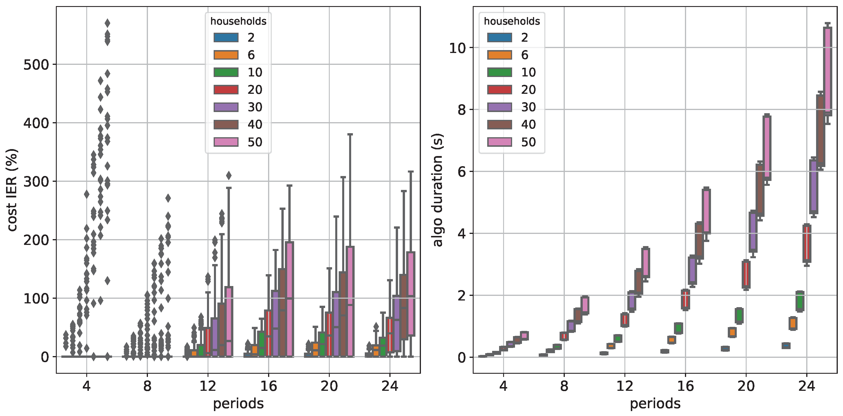
As can be seen in Table 3, the values increase with households and time periods. The peak power IER is not presented as it is constantly approximately zero. Figure 4 shows the spread of the quality measures cost IER and algo duration as boxplots.

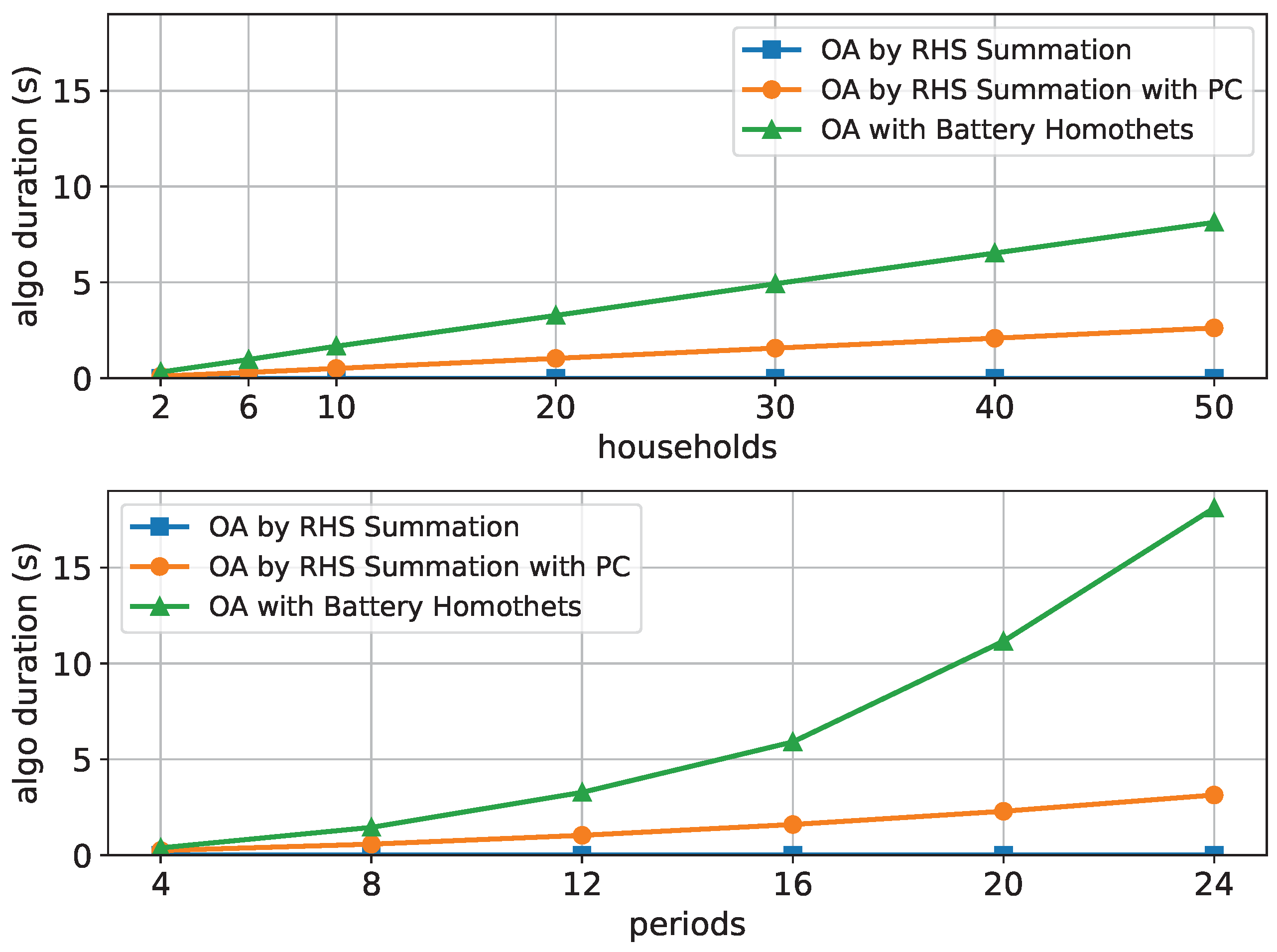
The computation time dependence is shown in Figure 5 for 12 time periods and increasing numbers of households at the top and 20 households and increasing numbers of time periods at the bottom. It can be seen that the algorithm OA by RHS Summation is the fastest and the algorithm OA with Battery Homothets is the slowest in both cases.

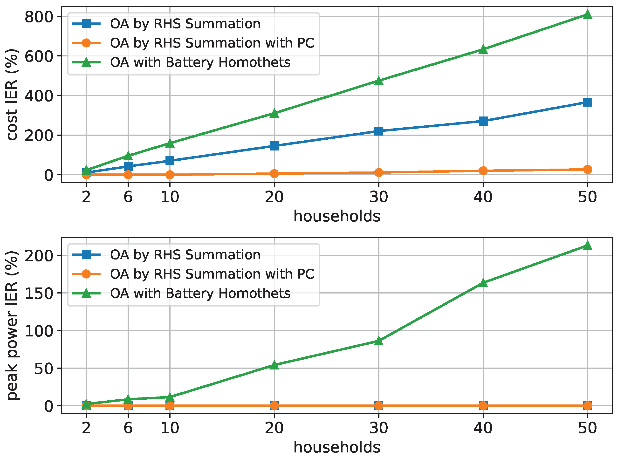
The quality criteria cost IER and peak power IER are shown with an increasing number of households and 12 time periods in Figure 6.

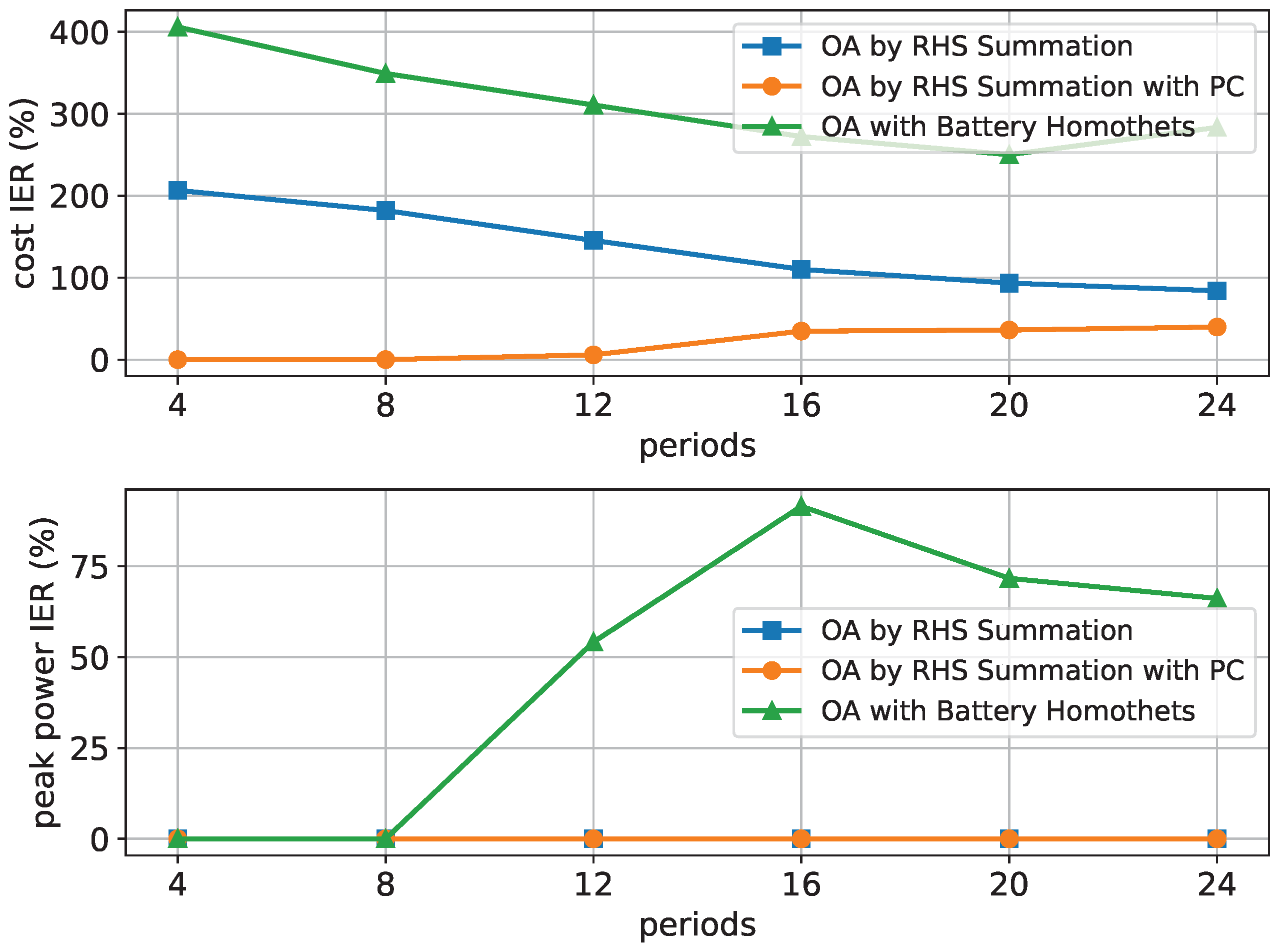
It can be seen that the OA with the Battery Homothets algorithm generally leads to the highest values while OA by RHS Summation with PC leads to the lowest values. The same is true when the number of households is fixed and the number of periods increases, as shown in Figure 7.

Although only selected columns and rows of the tables have been presented here, our results have shown that these observations are also valid for other fixed values of up to 50 households and 24 time periods.

5.2. Inner Approximations

This section presents the results for the inner approximations following the same format as the previous section.

The results for $N=10$ households and $M=8$ time periods are shown in

Table 4. Median values for inner approximations with $N=10$ and $M=8$.

Algorithms	Peak Power UPR (%)	Algo Time (s)	Cost UPR (%)
IA with Cuboid Homothets Stage 1	25.87	1.38	6.85
IA with Zonotopes Weighted	139.01	0.67	7.57
IA with Zonotopes $l_1$	156.32	0.74	7.73
IA with Cuboid Homothets Stage 0	25.87	0.08	8.77
IA with Zonotopes $l_2$	84.32	0.74	8.97
IA with Zonotopes $l_{\infty }$	0.00	2.12	10.89
IA by Battery Homothet Projection with LDR	0.00	3.77	18.61
IA with Battery Homothets	0.00	0.72	19.86
IA by Ellipsoid Projection with LDR	0.00	1.11	27.75
IA by Ellipsoid Projection	0.18	75.52	29.00

. For higher $(N,M)$ values some approximations were skipped because of the chosen computation time limit.

Table 4 shows that the algorithms IA with Cuboid Homothets Stage 0 and IA with Cuboid Homothets Stage 1 perform moderately well for the quality criteria cost UPR and peak power UPR. It is also evident that the ellipsoid-based algorithms perform poorly at cost UPR, but well for peak power UPR. Moreover, the ranking of the algorithms is different for different objectives which indicates that the approximations should be chosen according to the purpose.

For the algorithm IA with Cuboid Homothets Stage 1, the median cost UPR values for all households and time periods are given in

Table 5. Median cost UPR values for algorithm IA with Cuboid Homothets Stage 1.

Periods	4	8	12	16	20	24
Households
2	1.31	6.33	13.55	17.57	22.06	25.89
6	1.33	5.98	12.78	17.51	21.02	24.47
10	1.53	6.85	13.27	18.22	21.43	24.72
20	1.50	6.23	12.57	16.94	22.23	24.87
30	1.56	6.30	12.61	17.53	23.26	25.69
40	1.55	6.63	12.63	17.33	23.64	25.82
50	1.62	6.77	12.83	17.44	23.67	26.06

which shows increasing values with the number of time periods and the number of households.

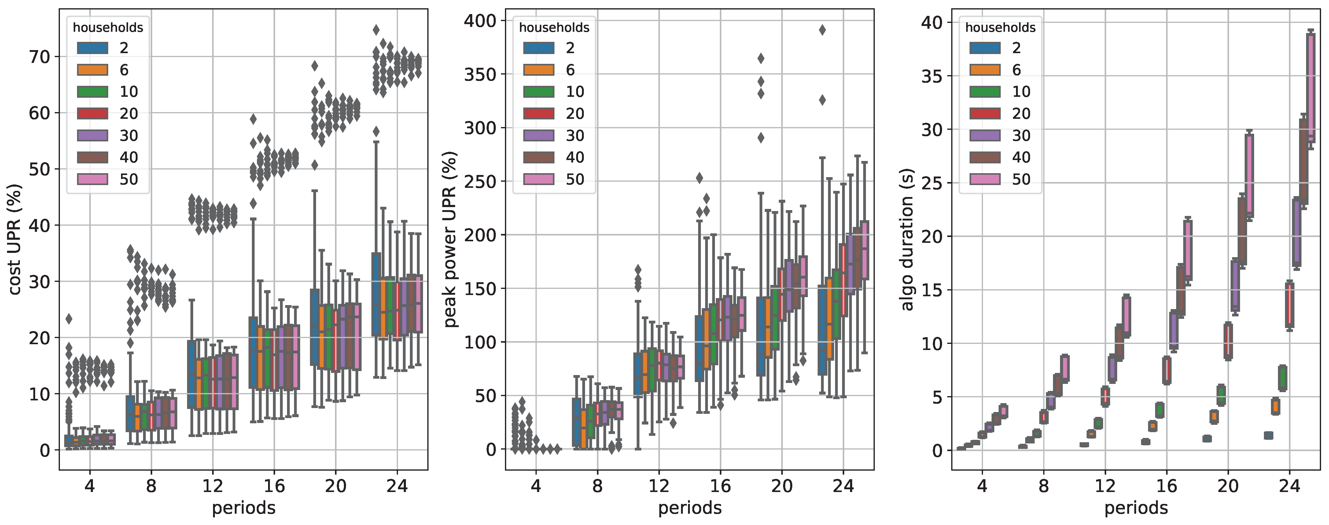
Figure 8 shows the spread of the quality measures cost UPR, peak power UPR and algo time as boxplots.

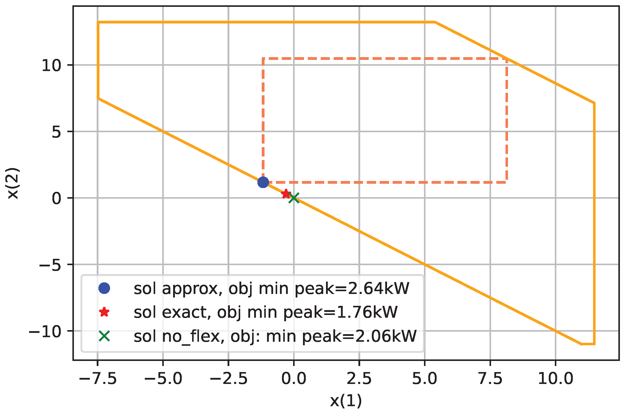
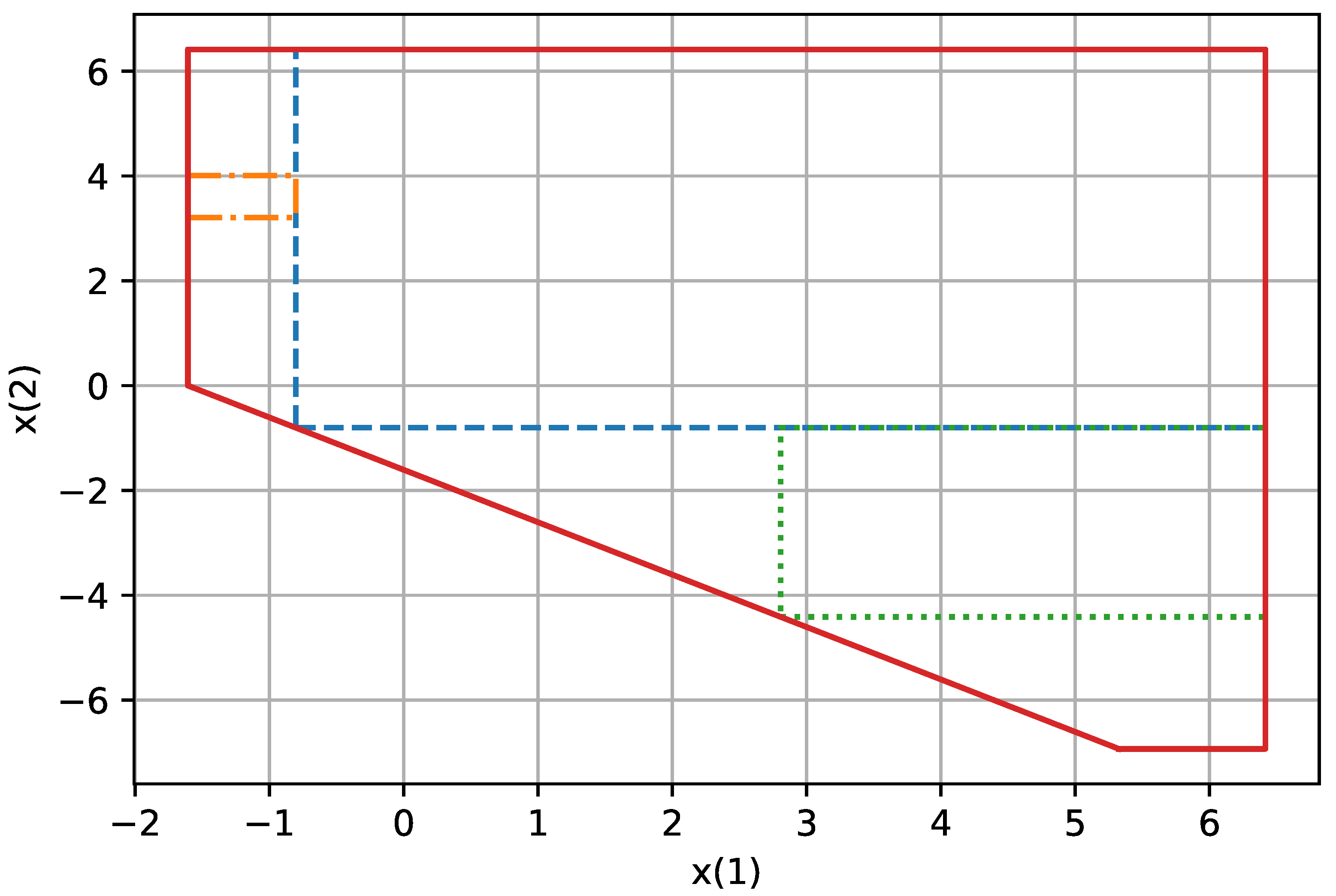
Note that there are UPR values beyond $100\%$, which indicates that the inner approximation gives larger values than without flexibility cf. Equation (45). Our results indicate that this is especially true when the peak power objective is used. The reason is that the inner approximation does not always contain the element corresponding to not using the flexibility, i.e., in our setting, the M-vector of zeros. Figure 9 shows this for two time periods and the algorithm IA with Cuboid Homothets Stage 0. We used $S_{\mathrm{end}}$ = $S_{0,i}$ for this experiment as for $S_{\mathrm{end}}$ = $\frac{S_{0,i}}{2}$, the problem described occurs in dimensions higher than two.

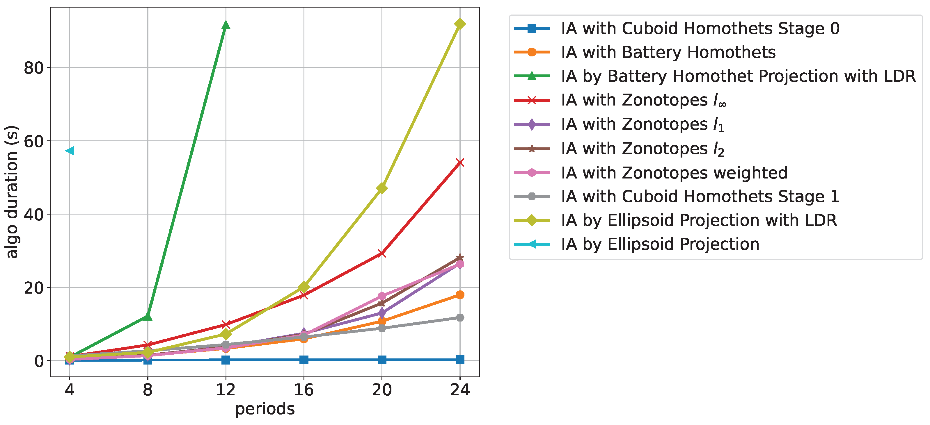
Figure 10 shows the computation time with increasing time periods for 20 households.

It can be seen that the approximations based on projection methods, i.e., IA by Ellipsoid Projection, IA by Ellipsoid Projection with LDR, and IA by Battery Homothet Projection with LDR exhibit the slowest computation times. The best computation times are achieved by the Cuboid Homothets algorithms of stage 0 followed by stage 1.

We observed the same order for an increasing number of households and fixed time periods. The only difference in this case is that all algorithms except for the projection-based ones exhibit linear increasing behavior.

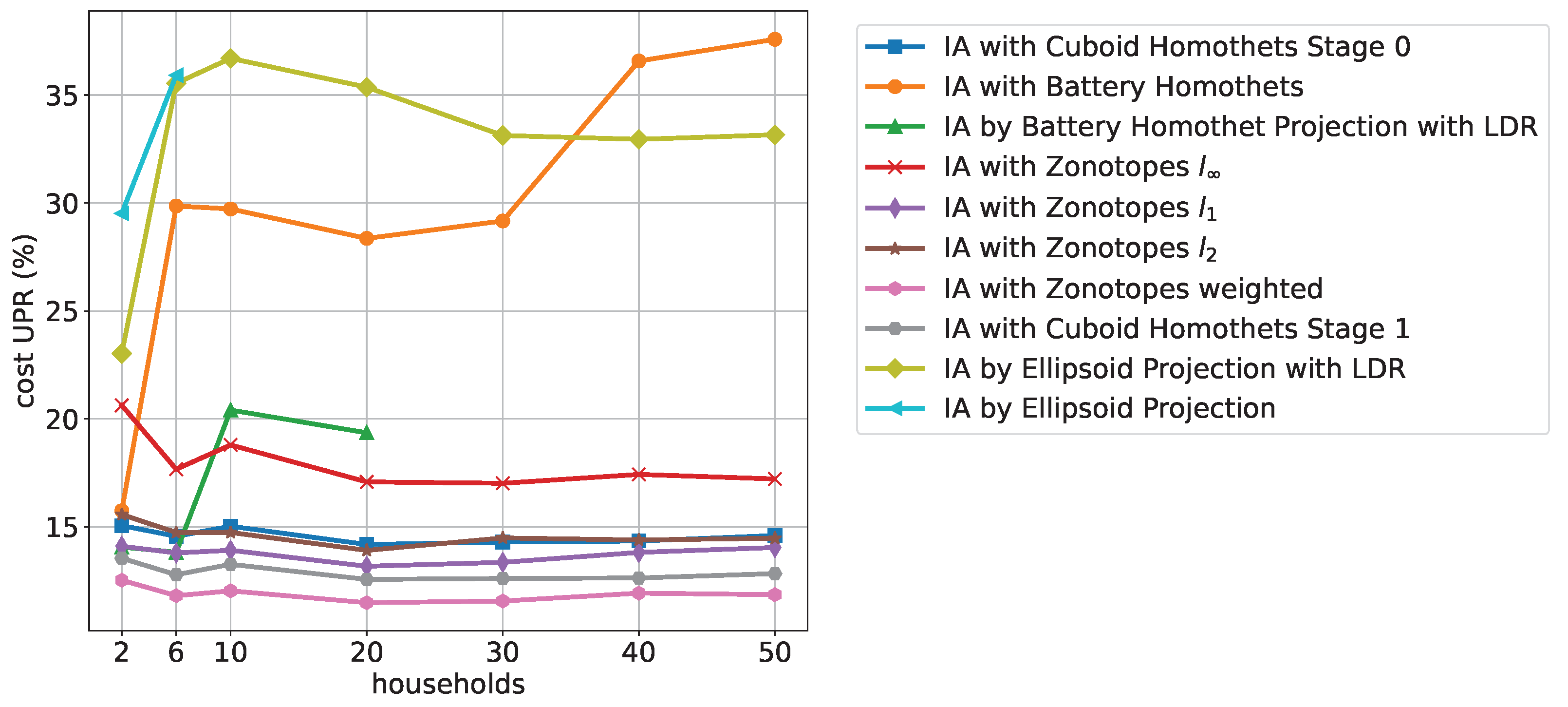
Figure 11 shows the cost UPR with increasing numbers of households for 12 time periods. It can be seen that the ellipsoid-based approximations generally do not perform well, while the zonotopes and the cuboid homothet-based approximations generally give good results. We found that for other fixed time periods, the order is maintained, except that the algorithms IA with Zonotopes $l_{\infty }$ and IA by Battery Homothet Projection with LDR improve:

For increasing time periods and a fixed number of households, the overall same order can be observed; however, with a linearly increasing dependence of cost UPR.

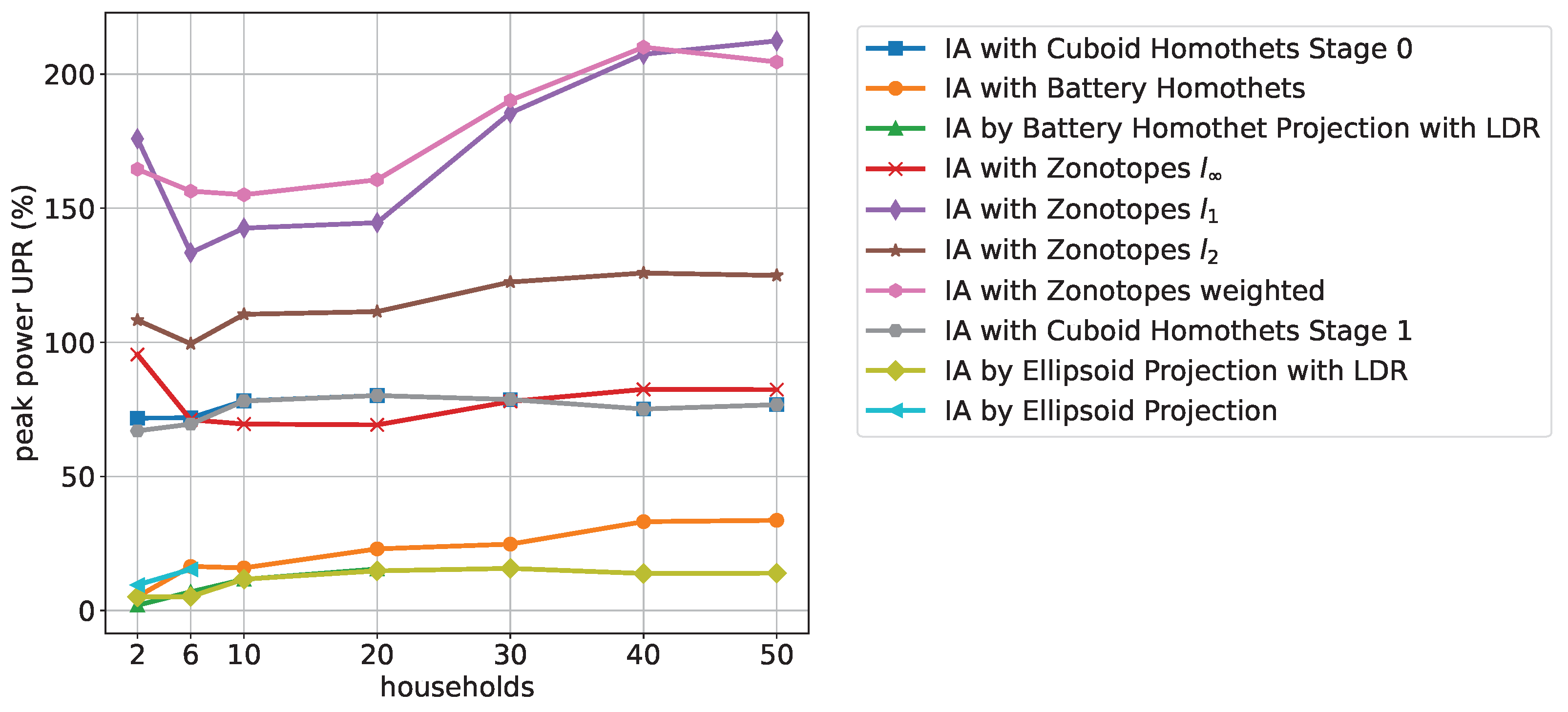
Figure 12 shows an improvement of the ellipsoid-based methods for peak power UPR compared to cost UPR.

The battery and ellipsoid-based algorithms perform best for peak power while the zonotope-based approximations do not perform well compared to the other algorithms. We found that this is also true for other values of fixed time periods, except that the Zonotope $l_2$ algorithm slightly improves. The overall order of best and worst performing algorithms is maintained for the fixed number of households with increasing time periods.

5.3. Overall Ranking

In practice, high N and M values are typically of greater interest. For this reason, we applied the following procedure to obtain an overall ranking of the inner and outer approximations:

• We only include approximations that returned results for all N and M values within the chosen computation time limit.
• For these approximations, the median values of the cost and peak power quality criteria were computed over all days, samples and $N\ge 30$ and $M\ge 16$ settings.

Table 6. Overall ranking: median overall quality criteria values for preselected approximations and N and M values, and in brackets, the rankings depending on approximation type (inner and outer) and objective function.

Algorithms	Cost UPR/IER (%)	Peak Power UPR/IER (%)
IA with Cuboid Homothets Stage 0	23.80 (4)	150.32 (4)
IA with Cuboid Homothets Stage 1	21.99 (3)	148.19 (3)
IA with Battery Homothets	43.97 (5)	32.15 (1)
IA with Zonotopes $l_1$	21.60 (2)	221.35 (6)
IA with Zonotopes $l_2$	23.80 (4)	112.66 (2)
IA with Zonotopes weighted	17.40 (1)	156.42 (5)
OA by RHS Summation	192.79 (2)	0.00 (1)
OA by RHS Summation with PC	76.32 (1)	0.00 (1)
OA with Battery Homothets	519.69 (3)	160.22 (2)

shows the remaining approximations, their median quality criteria values, and in brackets, the rankings depending on the approximation type (inner and outer) and objective function.

Table 6 shows the application-dependent performance of the inner approximations. Well-performing approximations for cost UPR do not perform well in peak power UPR and vice versa. For example, the algorithm IA with Zonotopes weighted ranks first in cost UPR but fifth in peak power UPR. Only mid-ranking algorithms, such as the cuboid-based algorithms, do not show such an extreme deviant behavior. Values above 100% for peak power UPR show that not using the flexibility is more efficient than using the approximation which makes the approximation useless for that purpose. This is the case for all inner approximations expect IA with Battery Homothets. For outer approximations, the algorithm OA by RHS Summation with PC ranks first for both cost and peak power IER. However, for cost IER, approximately 75% of the flexibility energy needs to be purchased as imbalance energy, which is generally expensive.

6. Conclusions

In this paper, we investigated several published approximation methods for aggregating demand-side flexibilities given by energy storage devices. The different approximations were described and compared with respect to communication and computation efforts. Furthermore, we defined and evaluated novel quality criteria to assess the quality of the approximations for their use in practice. Finally, the evaluation framework was made publicly available such that researchers can compare future approximations with the current state of the art.

The evaluation results show that the projection-based algorithms exhibit the highest computation times. The ellipsoid-based algorithms showed the lowest communication effort. For inner approximations, we suggest application-dependent-choices, cf. Table 6. The best results were obtained for outer approximations when the OA by RHS Summation with PC was used. We conclude that not one of the presented approximations fits all purposes.

Only the cuboid homothets algorithm can configure its accuracy, namely by increasing the number of stages. This, however, is accompanied by an exponential increase in computational effort.

We found a crucial weakness of many inner approximations, especially when minimum peak power is considered, namely that they do not always contain the element corresponding to not using the flexibility and may therefore lead to solutions that perform worse compared to the case where no flexibility is available. Thus, future work should yield inner approximations that overcome this deficiency in all cases.

Our evaluation model is extendable in several ways. First, renewable energy generation can be subsumed into the demand profiles. The inclusion of self-discharge rates $<1$ changes the submatrix $\Gamma$ in Equation (9) and results in possibly different A matrices for different households. This can be transformed in our model with equal A-matrices by introducing redundant constraints through PC, cf. [17]. Finally, as TCLs can be described by battery models with a self-discharge rate $<1$, they can also be modeled with different A-matrices, cf. [3]. Future work should investigate how an increased diversity of individual flexibilities influences the accuracy of aggregation approximations. Furthermore, the control of reactive power, e.g., by inverters, is becoming more important with the increasing number of PV systems in smart grids. Therefore, future studies should consider the flexibility of active and reactive power simultaneously.

We did not include charging and discharging efficiencies $<1$ because if simultaneous charging and discharging is not allowed, their inclusion leads to non-convex sets. This aspect of real storage devices as well as uncertainties in data and parameters and model predictive control approaches should also be considered in future work.