
Verification of the Parallel Transport Codes Parafish and AZTRAN with the TAKEDA Benchmarks

 ,
,  ,
,  and
and
Abstract
:1. Introduction
2. Parallel Neutron Transport Codes under Development
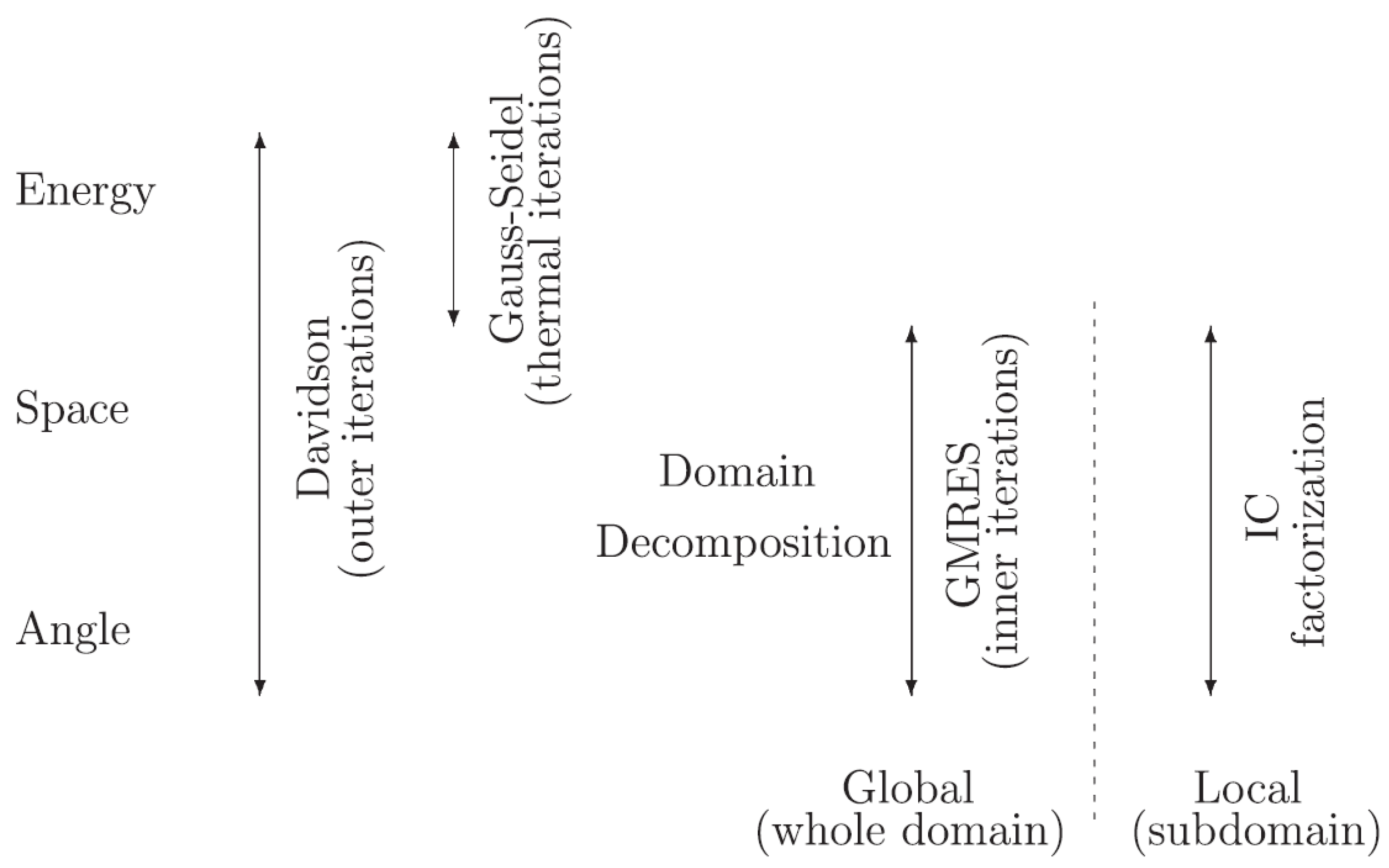
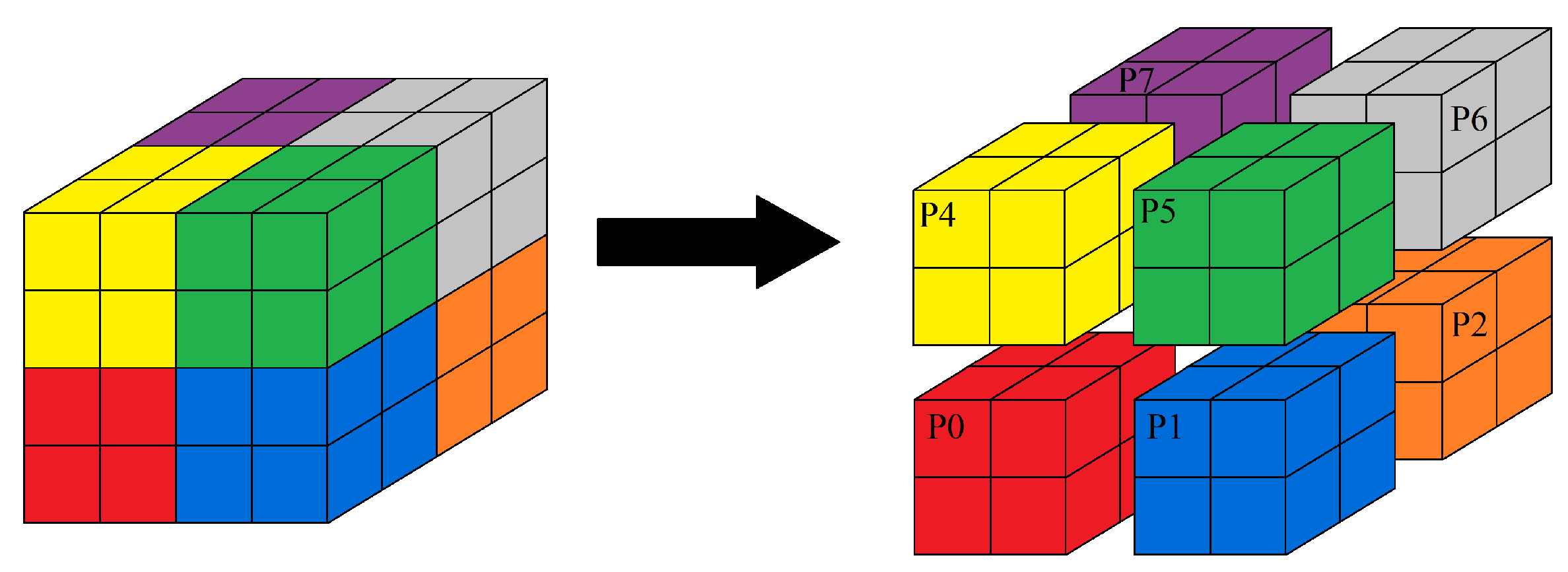
2.1. Parafish
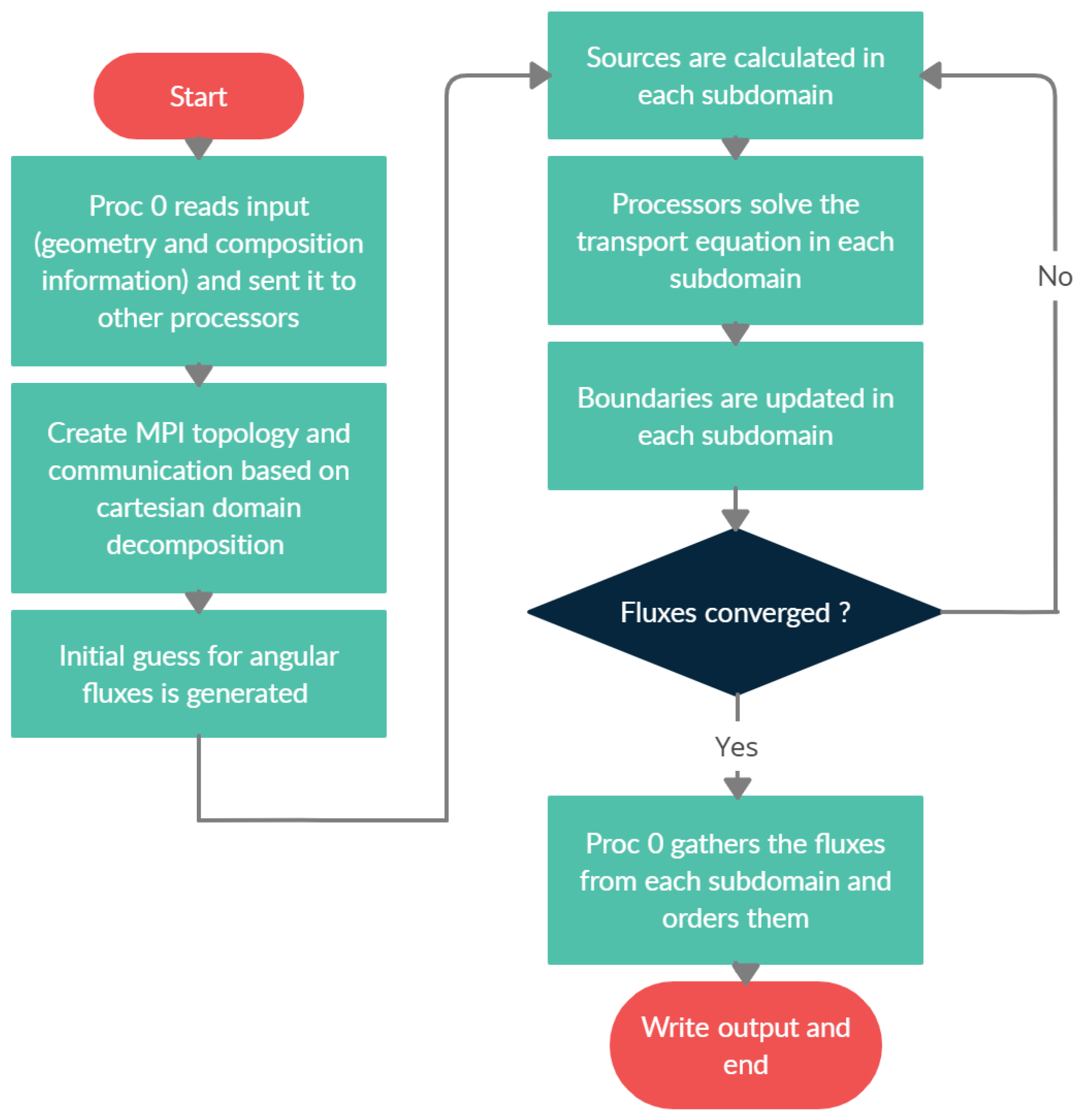
2.2. AZTRAN
3. TAKEDA Benchmarks Description
3.1. Model 1 (Small LWR Core)
3.2. Model 2 (Small FBR Core)
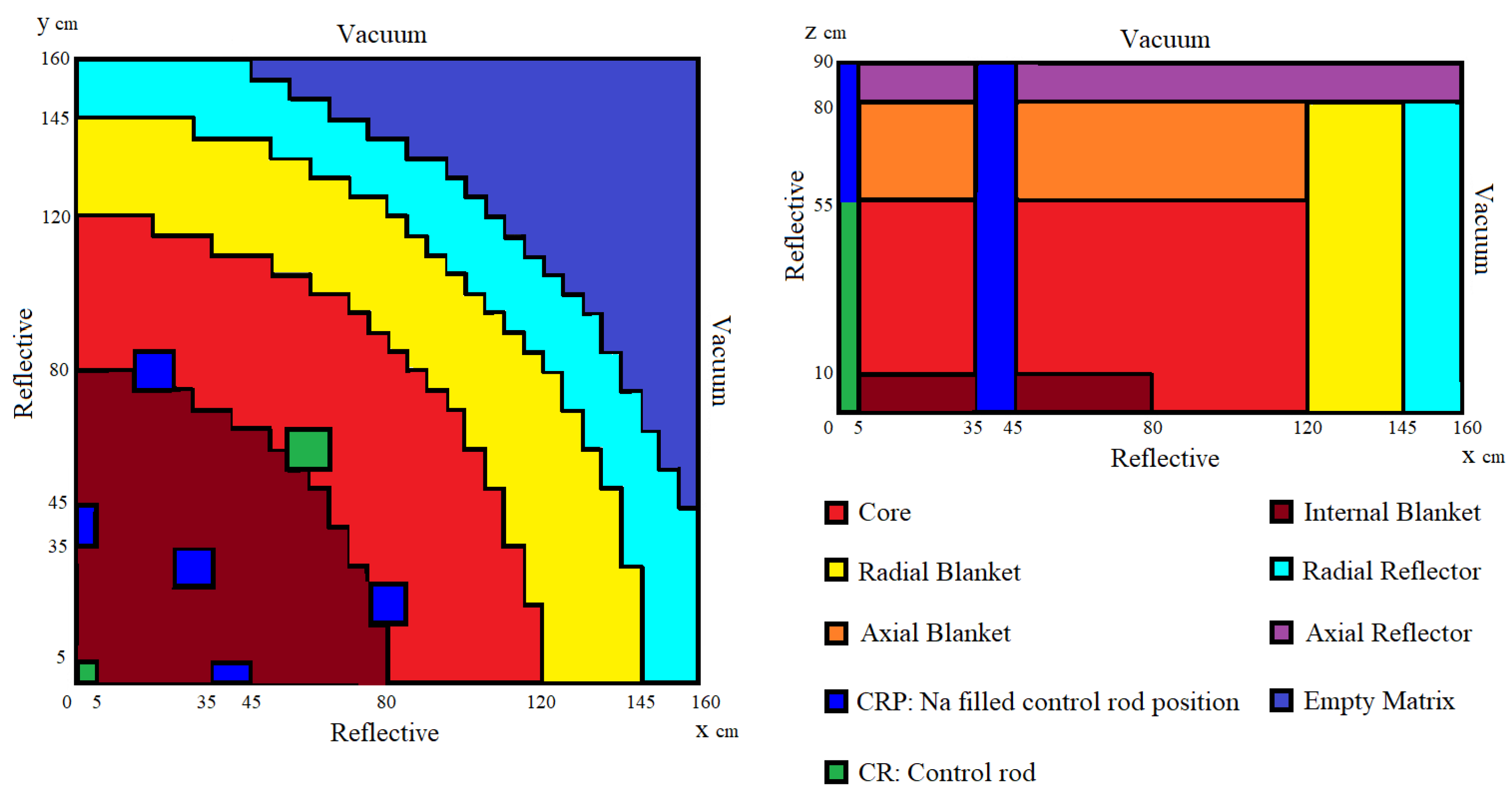
3.3. Model 3 (Axially Heterogeneous FBR Core)
4. Numerical Results
4.1. Small LWR Core
4.2. Small FBR Core
4.3. Axially Heterogeneous FBR Core
5. Parallel Scaling
6. Conclusions and Outlook
Author Contributions
Funding
Institutional Review Board Statement
Informed Consent Statement
Data Availability Statement
Acknowledgments
Conflicts of Interest
References
- Fletcher, J.K. The Solution of the Multigroup Neutron Transport Equation Using Spherical Harmonics. Nucl. Sci. Eng. 1983, 84, 33–46. [Google Scholar] [CrossRef]
- Lewis, E.E.; Miller, W.F. Computational Methods of Neutron Transport; Wiley: Hoboken, NJ, USA, 1984. [Google Scholar]
- Lathrop, K.D. Ray effects in discrete ordinates equations. Nucl. Sci. Eng. 1968, 32, 357–369. [Google Scholar] [CrossRef]
- Morel, J.; Wareing, T.; Lowrie, R.; Parsons, D. Analysis of ray-effect mitigation techniques. Nucl. Sci. Eng. 2003, 144, 1–22. [Google Scholar] [CrossRef]
- Smith, M.A.; Lewis, E.E.; Shemon, E.R. DIF3D-VARIANT 11.0: A Decade of Updates; Argonne National Lab. (ANL): Argonne, IL, USA, 2014. [Google Scholar] [CrossRef]
- Ziver, A.K.; Shahdatullah, M.S.; Eaton, M.D.; Oliveira, C.R.E.; Umpleby, A.P.; Pain, C.C.; Goddard, A.J.H. Finite element spherical harmonics (PN) solutions of the three-dimensional Takeda benchmark problems. Ann. Nucl. Energy 2005, 32, 925–948. [Google Scholar] [CrossRef]
- Alcouffe, R.E.; Baker, R.S.; Dahl, J.A.; Turner, S.A.; Ward, R. PARTISN: A Time-Dependent, Parallel Neutral Particle Transport Code System; LA-UR-08-07258; Los Alamos National Laboratory: Los Alamos, NM, USA, 2008. [Google Scholar]
- Seubert, A.; Velkov, K.; Langenbuch, S. The time-dependent 3-d discrete ordinates code TORT-TD with thermal-hydraulic feedback by ATHLET models. In Proceedings of the Physor 2008, Interlaken, Switzerland, 14–19 September 2008. [Google Scholar]
- Criekingen, S.V.; Nataf, F.; Havé, P. PARAFISH: A parallel FE–PN neutron transport solver based on domain decomposition. Ann. Nucl. Energy 2011, 38, 145–150. [Google Scholar] [CrossRef]
- Criekingen, S.V. A Non-Conforming Generalization of Raviart-Thomas Elements to the Spherical Harmonic form of the Even-parity Neutron Transport Equation. Ann. Nucl. Energy 2006, 33, 573–582. [Google Scholar] [CrossRef] [Green Version]
- Subramanian, C.; Criekingen, S.V.; Heuveline, V.; Nataf, F.; Havé, P. The Davidson method as an alternative to power iterations for criticality calculations. Ann. Nucl. Energy 2011, 38, 2818–2823. [Google Scholar] [CrossRef]
- Nakamura, S. Computational Methods in Engineering and Science: With Applications to Fluid Dynamics and Nuclear Systems; Wiley: New York, NY, USA, 1977. [Google Scholar]
- Saad, Y.; Schultz, M.H. GMRES: A generalized minimal residual algorithm for solving non-symmetric linear systems. SIAM J. Sci. Statis. Comput. 1986, 7, 856–869. [Google Scholar] [CrossRef] [Green Version]
- Lions, P.L. On the Schwarz Alternating Method III: A variant for Nonoverlapping Subdomains. In Third International Symposium on Domain Decomposition Methods for Partial Differential Equations; SIAM: Philadelphia, PA, USA, 1990; pp. 202–223. [Google Scholar]
- Gomez-Torres, A.; del Valle-Gallegos, E.; Duran-Gonzalez, J.; Rodriguez-Hernandez, A. Recent developments in the neutronics codes of the AZTLAN platform. In Proceedings of the International Congress on Advances in Nuclear Power Plants ICAPP, Abu Dhabi, United Arab Emirates, 16–20 October 2021. [Google Scholar]
- Duran-Gonzalez, J.; del Valle-Gallegos, E.; Reyes-Fuentes, M.; Gomez-Torres, A.; Xolocostli-Munguia, V. Development, verification, and validation of the parallel transport code AZTRAN. Prog. Nucl. Energy 2021, 137, 103792. [Google Scholar] [CrossRef]
- Hennart, J.P.; del Valle, E. Nodal finite element approximations for the neutron transport equation. Math. Comput. Simul. 2010, 80, 2168–2176. [Google Scholar] [CrossRef]
- Yavu, M.; Larsen, E.W. Iterative Methods for Solving x-y Geometry SN Problems on Parallel Architecture Computers. Nucl. Sci. Eng. 1992, 112, 32–42. [Google Scholar] [CrossRef]
- Takeda, T.; Ikeda, H. 3D Neutron Transport Benchmarks. Technical Report OECD/NEA, Committee on Reactor Physics (NEACRP), OSAKA University, NEACRP-L-330. 1991. Available online: https://www.oecd-nea.org/upload/docs/application/pdf/2020-01/neacrp-l-1990-330.pdf (accessed on 24 December 2021).
- Takeda, T.; Ikeda, H. 3D neutron transport benchmarks. Nucl. Sci. Technol. 1991, 28, 656–669. [Google Scholar] [CrossRef]
- Fletcher, J.K. MARK/PN A Computer Program to Solve the Multigroup Transport Equation; RTS-R-002; AEA: Risley, UK, 1988. [Google Scholar]


| Code | Case 1 | Case 2 | CR-Worth |
|---|---|---|---|
| Monte-Carlo | 0.97780 | 0.96240 | |
| Parafish | 0.97686 | 0.96249 | |
| [96 pcm] | [9 pcm] | [7.3%] | |
| AZTRAN | 0.97758 | 0.96276 | |
| [22 pcm] | [37 pcm] | [4.2%] |
| Code | Case 1 | Case 2 | CR-Worth |
|---|---|---|---|
| Monte-Carlo | 0.97310 | 0.95890 | |
| Parafish | 0.97511 | 0.96143 | |
| [206 pcm] | [263 pcm] | [2.0%] | |
| AZTRAN | 0.97460 | 0.96079 | |
| [154 pcm] | [197 pcm] | [0.6%] |
| Code | Case 1 | Case 2 | Case 3 | CR-Worth | CRP-Worth |
|---|---|---|---|---|---|
| Monte-Carlo | 0.97080 | 1.00050 | 1.02140 | ||
| Parafish | 0.97340 | 1.00230 | 1.02290 | ||
| [267 pcm] | [179 pcm] | [146 pcm] | [3.2%] | [0.9%] | |
| AZTRAN | 0.97254 | 1.00175 | 1.01738 | ||
| [179 pcm] | [124 pcm] | [393 pcm] | [1.9%] | [24.6%] |
Publisher’s Note: MDPI stays neutral with regard to jurisdictional claims in published maps and institutional affiliations. |
© 2022 by the authors. Licensee MDPI, Basel, Switzerland. This article is an open access article distributed under the terms and conditions of the Creative Commons Attribution (CC BY) license (https://creativecommons.org/licenses/by/4.0/).
Share and Cite
Duran-Gonzalez, J.; Sanchez-Espinoza, V.H.; Mercatali, L.; Gomez-Torres, A.; Valle-Gallegos, E.d. Verification of the Parallel Transport Codes Parafish and AZTRAN with the TAKEDA Benchmarks. Energies 2022, 15, 2476. https://doi.org/10.3390/en15072476
Duran-Gonzalez J, Sanchez-Espinoza VH, Mercatali L, Gomez-Torres A, Valle-Gallegos Ed. Verification of the Parallel Transport Codes Parafish and AZTRAN with the TAKEDA Benchmarks. Energies. 2022; 15(7):2476. https://doi.org/10.3390/en15072476
Chicago/Turabian StyleDuran-Gonzalez, Julian, Victor Hugo Sanchez-Espinoza, Luigi Mercatali, Armando Gomez-Torres, and Edmundo del Valle-Gallegos. 2022. "Verification of the Parallel Transport Codes Parafish and AZTRAN with the TAKEDA Benchmarks" Energies 15, no. 7: 2476. https://doi.org/10.3390/en15072476
APA StyleDuran-Gonzalez, J., Sanchez-Espinoza, V. H., Mercatali, L., Gomez-Torres, A., & Valle-Gallegos, E. d. (2022). Verification of the Parallel Transport Codes Parafish and AZTRAN with the TAKEDA Benchmarks. Energies, 15(7), 2476. https://doi.org/10.3390/en15072476