Article

Economic and Environmental Assessment Using Two Renewable Sources of Energy to Produce Heat and Power for Industrial Applications

by
Guillermo Martínez-Rodríguez
1,*,
Juan-Carlos Baltazar
2,
Amanda L. Fuentes-Silva
1 and
Rafael García-Gutiérrez
3
1
Department of Chemical Engineering, University of Guanajuato, Guanajuato 36050, Mexico
2
Energy Systems Laboratory, TEES, 7607 Eastmark Drive, College Station, TX 77840, USA
3
Physics Research Department, Universidad de Sonora, Hermosillo 83000, Mexico
*
Author to whom correspondence should be addressed.
Energies 2022, 15(7), 2338; https://doi.org/10.3390/en15072338
Submission received: 28 February 2022 / Revised: 19 March 2022 / Accepted: 21 March 2022 / Published: 23 March 2022

Abstract

:
Economic criteria have prevailed in studies on integration of renewable energies. Tons of dangerous emissions are emitted by a biomass fuel, causing negative impacts over atmosphere and health. Current research proposes Pinch Analysis of solar thermal energy and the joint use of biomass (sugarcane bagasse) to produce heat and power in a Caribbean sugar mill; measuring emissions like: carbon oxide C O , carbon dioxide C O 2 , dinitrogen monoxide N 2 O , nitrogen oxides N O x , sulfur oxides S O x , non-methane volatile organic compounds NMVOC, methane C H 4 , and particulate matters, to have a global and clear view of the impacts of biomass as a renewable fuel. Variables like kWh cost, the installation and device area of renewable energy, and greenhouse gas emissions, are analysed to assess the effect on the integration final design, the target of which is to control the use of biomass. It is possible to produce an economically competitive integration design of solar system L C O E t h   s o l a r = 0.0636 USD/kWh, L C O E e l e = 0.1392 USD/kWh), zero greenhouse gases emissions ( Δ T m i n r e w = 7   ° C ), and deletion of 378,711.53 t/year of C O 2 and 9567.56 t/year of solid particles. There are many possibilities that can implemented; in one of them, bagasse burning is reduced by 30% and the solar collector network for required power production is reduced by 68%.

1. Introduction

Transition towards renewable energies is a global topic in constant evolution with objectives established a priori. In general, the renewable kWh cost is the parameter that defines the installation of clean technology. There are other parameters that must be considered, including simple payback time, levelised cost and occupied area of the renewable device. All of these are of relevance during design, installation, and operation of renewable systems.
There are some papers related to renewable energy integration in industrial processes. Martínez-Rodríguez et al., in 2019, [1] carried out the solar thermal energy integration to dairy process, supplying the total heat load. Simple payback times less than three years were calculated. Valderrama et al. (2020) [
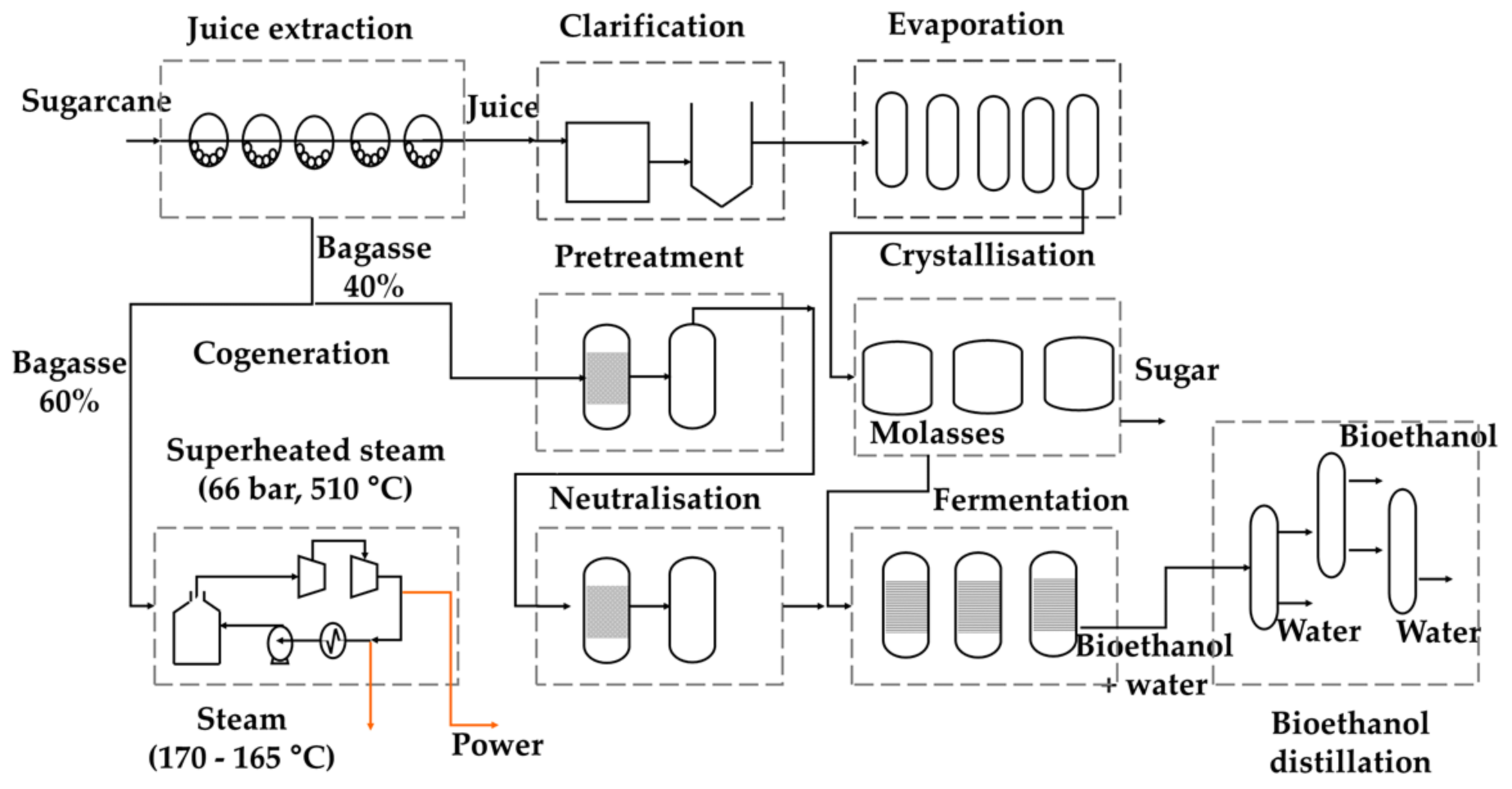
2] used 60% of sugarcane bagasse to produce heat and power in a bioethanol production process (1G and 2G). Taking account of the variability of some renewable energies like solar, renewable hybrid systems have been proposed that seek to give confidence and certainty to the energy systems of the industrial sector. Da Silva et al. (2020) [3] studied the energetic aspects related with the adoption of a hybrid system compound by a parabolic trough collector solar field (PTC), a biomass burner (biomass: Eucalyptus grandis wooden briquettes), an intermediate thermal oil circuit, a regenerative organic Rankine cycle (ORC), and an absorption cooling system to deliver the energy demand of a small industrial plant in Brazil. It considered the solar energy like the primary source and the biomass as secondary ones. Tsimpoukis et al., 2021, [4] analysed, in energetic terms, the concept of a trigeneration system of super-critical C O 2 to cover the needs of a cold store in Athens, with simultaneous production of electricity and heating. This system took advantage of captured solar energy by PTC and biomass (dry straw) as a supplemental energy source to increase the temperature of C O 2 at high pressure in a turbine that is coupled to a generator. The study analysed different scenarios. Simple payback time was four years for solar collectors, and 13.5 years for the biomass boiler. The financial savings were equivalent to EUR 542,000 and EUR 22,900 for the estimated useful life of the project. In the works mentioned above, biomass had a role as a secondary energy or backup system, to buffer the variability of the solar resource.
There is research about the economic and environmental advantages in using biomass co-fired with coal for the reduction of net emissions of C O 2   [5], because there is a balance between the amount of carbon dioxide absorbed by plants while they are growing, and the amount released during biomass burning; an activity that is carried out at an industrial level in European countries with relative success [6], since the use of fuels obtained from biomass is considered a sustainable energy source, and they are highly recommended as carbon neutral fuels [7]. However, the common theme of biomass burning is its significant contribution in relevant pollutants in addition to C O 2 , such as S O 2 and black carbon, to name a few. So, the use of biomass as a renewable fuel must be approached from a comprehensive point of view when evaluating its impacts on the global environment and climate region [7].
The burning of some biomass residues also produces toxic compounds, including polychlorinated dibenzo-p-dioxins and dibenzofurans (PCDD/F), which are listed as persistent organic pollutants and have been linked to adverse risks to human health that should not be ignored [8]. These health risks include chloracne, immunotoxicity, endocrine disruptors, mutagenicity, and carcinogenicity [9,10,11]. In the United States, more than 14% of PCDD/F air emissions are from controlled sources of the combustion of wood used for heat and power generation, which is much higher than waste incineration and coal combustion [12]. Small-scale industrial combustion was also found to be the main source of PCDD/F emission in Guangzhou, China [13]. The annual estimate of PCDD/F emitted by biomass combustion in the industrial sector was approximately 208 g of l-EQT (international toxic equivalency factors) in China, which represents 2% of total national emissions, annually [8].
S O 2 is a widely cited air pollutant that has important effects on ecosystems, human health, and the climate [14]. Total emissions originating from all sources, including biomass, reached 105.4 Tg in 2014, with 43% coming from power plants and 35% from industry [15]. S O 2   emissions are not negligible, especially in many developing countries and certain developed countries [16]. In the US, France, Germany, Finland, India and other Asian countries, contributions of S O 2   to biomass are increasing [17].
World sugar production is expected to recover from the current fall and rise by approximately 16%, this projected upturn in the economy of the sugar sector will promote an increase in emissions resulting from the burning of biomass.
According to the Intergovernmental Panel on Climate Change, regarding global warming impacts of 1.5 °C [18], to accomplish the zero C O 2   emissions goal in 2050, an unprecedented energy transition is imperative, in all sectors of society. The goal requires the transition from fossil fuels to clean energies to reduce or eliminate the generation of GHG emissions. The industrial sector, in particular, must decrease their direct C O 2 emissions, by 2050, by 6 Gt (66% of current levels), and limit energy use to 200 EJ (40% below current levels) [5]. There is a well-established industry of burning biomass to produce energy across the world. However, it must be borne in mind that regardless of the type of biomass used, gases and particulate matters are emitted in large, uncontrolled quantities, which maintain high levels of carbon in the environment and persistent pollution.
The purpose of this research work was to supply the energy of an industrial process through an energy system design with controlled emissions, through the incorporation of solar energy and biomass. The emissions caused by use of natural gas are compared against those caused by the burning of sugarcane bagasse, since it is generally perceived that the latter generates fewer emissions, compared to other fossil sources. The results indicate that the burning of sugarcane bagasse generates a greater variety and quantity of emissions than natural gas. There are scenarios in which it is possible to integrate an energy system based on solar thermal energy that meets technical, environmental, and economic criteria, which guarantee the total supply of energy for an industrial process. Alternatively, there are scenarios where it is convenient to combine the use of biomass and solar thermal energy, where the former is used setting a priori control of emissions. When the objective is to reach a solar fraction of 0.5, the area of the solar collector network is reduced by 48%. There is a direct relationship between the solar fraction, the emissions, and the area of the solar field.

2. Integration of Solar Energy and Reduction of Burning Biomass

The industrial sector uses the bagasse mainly like backup. In bagasse burning, the generation of dioxins, particulate matters (PM), and volatile organic compounds (VOC) is common. These gases are extremely dangerous for human health [11]. In the case study of bioethanol processes 1G and 2G, described by Valderrama et al. [2], the bagasse is burned for heat and power cogeneration.
This study shows how the integration of solar energy could be used to substitute in a partial or total way the use of bagasse as a biofuel, and how the integration of solar energy controls and reduces the generation of dangerous gases from biomass burn. An economic analysis, associated with the amounts of pollutants generated by biomass burning, shows that biomass can be replaced by solar thermal to produce heat and power, and thus, reducing biomass burning is feasible. The caloric value of sugarcane bagasse taken in this study is 8477.4 J/kg [19] to estimate the heat load produced by the boiler (in Table 1).

2.1. Bioethanol Production Process (1G and 2G) from Sugarcane

The case study is a sugar mill located in Valle del Río Cauca, Colombia. To produce 38 ton/h per day and 12,654.5 kg/h of bagasse, 40% of bagasse is returned to the process, the rest is used to deliver the energy required by the process. The sugar mill operates 18 h/day [20] and produces 29,023.95 kg/h of superheated steam at 510 °C and 66 bar with an efficiency of 64%, to produce electricity in a turbine with a power of 3147.30 kW and with an isentropic efficiency of 69.9%. The steam produced is destined for the stages of evaporation and crystallisation, in addition to the generation of power.
Bioethanol process unit operation is shown in Figure 1. First, cane juice is extracted by grinding the raw material; at this stage, bagasse is obtained as a residue. The juice extracted in the first stage is clarified by adding lime and flocculants, this allows neutralisation of the juice and eliminates the solids and impurities present in it. Clarified juice goes to the evaporation stage, where water is extracted and then concentrated until a molasses is obtained. In the crystallisation stage, molasses is converted into sugar grains by vacuum containers of simple effect and the addition of heat, but it is necessary that the mixture goes through a centrifugation process to separate the grains from the molasses. This molasses goes to the fermentation stage in conjunction with the liquor obtained from bagasse. Then, this fermented broth is distilled, and bioethanol is obtained.
Conventional distillation is used in the purification stage, followed by dehydration with molecular sieves. This stage consists of three distillation columns: degassing, rectification, and separation of aldehydes; thus, achieving the production of bioethanol with a concentration of 99%. To design heat recovery network, Table 2 shows data from hot and cold process streams, which can exchange energy. It also presents the inlet and outlet temperatures of the streams, their heat capacity flow rate, and the individual heat transfer coefficient, h .

2.2. Solar Thermal Energy Integration

Using the Pinch Analysis, it is possible to identify the minimum hot utility and multiple hot utility to increase the use of solar thermal energy. Targets can also be set for the utility load at various levels. Utility levels supplied to the process may be a part of a centralised site-wide utility system. The grand composite curve (GCC) provides a convenient tool for setting the targets for the multiple utility levels. Δ T m i n defines these ones looking to maximise the use of low-temperature solar thermal energy.

2.3. Low-Temperature Solar Thermal Energy

According to the Solar Payback Project [21], 32% of global energy use is in the industrial sector, and 74% of these energetic needs in industry are from heat. One third of this heat is covered by low-temperature heat. Almost all the heat process demand required are in temperature ranges that could be supplied a solar thermal system. Pursuant to the recently published Renewables 2021 Global Status Report by REN21, thermal uses in 2018, which include water and space heating, space cooling, and industrial heat processes, accounted for more than half (51%) of total final energy consumed.
Identifying the minimum hot utility and multiple utility levels, the next step is to design the solar collector network following the method proposed by Martínez-Rodríguez et al. [1]. The final design arrangement must deliver the temperature using collectors connected in series, and the heat load, using series connected in parallel. This method also considers heat storage to guarantee the heat load at the level of target temperature. Lizárraga-Morazán et al., 2020 [22], furnished a cost equation to calculate the investment of a network of solar collectors. The solar thermal heat is used to supply the solar heat load, and also to deliver the solar energy required on the evaporator to produce power through the organic Rankine cycle (ORC).

2.4. Power Cycle: Organic Rankine Cycle (ORC)

The organic Rankine cycle is a mature technology, it has low maintenance costs, a high degree of automation, and employs more compact equipment compared to water-steam cycle technology, making it the best commercial solution available for electricity production [23]. ORC has shown to be a good solution for small- and medium-scale generation, as well as decentralised generation [23].
The selection of the working fluid requires a thermodynamic study of the operating conditions, such as low pressure and critical temperature, low specific volume, or high thermal conductivity, among others, to increase the operation of the ORC. It seeks to improve the mechanisms of heat transfer to reduce the size of the equipment, save energy and costs. In addition, the toxicity, flammability, availability, thermal efficiency, and compatibility of materials must be considered [24]; working fluids with low environmental impact and a high level of safety must be evaluated.
Ozone depletion potential and the global warming potential (GWP) index are the main parameters to be considered.
Figure 2 displays the proposal of how to supply the heat load to the evaporator at 105 °C. We used a network of low-temperature solar collectors, designed following the method proposed by [1].
In this stage, the heat required by the evaporator ( Q e v a ) is delivered by the solar collector network and calculated following Equation (1).
Q e v a = m ˙ f w h 3 h 2 .  
where m ˙ f w is the mass flow of the working fluid, and h 2 and h 3 (kJ/kg) are the enthalpies at the inlet and outlet of the evaporator. Assuming an isentropic turbine efficiency η i s o of 69.9%, the enthalpy at the turbine outlet ( h 4 ) is calculated using Equation (2).
h 4 = h 3 η i s o h 3 h 4 ,   i s o
The work produced by the turbine, W t u r b , is calculated as a function of the turbine efficiency using Equation (3).
W t u r b = m ˙ f w h 3 h 4 η t u r b
where η t u r b is the efficiency of the turbine. A turbine efficiency of 87% was taken [3].
Condenser heat load Q c o n is obtained from Equation (4).
Q c o n = m ˙ f h 4 h 1 .  
The operating pressure of the condenser is assumed to be 1 atm. h 1 is the enthalpy at the condenser outlet, in kJ/kg. The power consumed by the pump to move the fluid is obtained with the following Equation (5).
W p u m p = m ˙ f v f P 2 P 1 η p u m p  
where η p u m p is the efficiency of the pump. An efficiency of 85% for the pump was taken [3].
The net power output of the system, W n e t , is calculated with Equation (6).
W n e t = W t u r b η g e n W p u m p
where η g e n is the generator efficiency. An efficiency of 89% for the generator was taken [3].
Finally, the ORC efficiency ( η O R C ) , in Equation (7), is obtained by using Equations (4) and (6).
η O R C = W n e t Q c o n
To design the evaporator and condenser of the Rankine cycle, the general design in Equation (8) was used.
Q h x = U A Δ T L M T D
where U is the overall heat transfer coefficient, in kW/m2 °C, A is the heat exchange area, in m2, and Δ T L M T D is the logarithmic mean temperature difference between hot and cold streams that exchange heat, in °C. In this work, the reported values of U , such as 1.2 and 1.1 kW/m2 °C, were taken for the estimation of the exchange area of the evaporator and condenser, respectively [25]. The costs of the equipment that make up the Rankine cycle were calculated using the equations [26] reported in Table 3.

2.5. Quantification of Bagasse Emission Pollution

Gil-Unday et al. [27] reported real values of pollutants emitted by bagasse in tons emitted per GWh. Table 4 shows the indices of gas emissions generated. The results correspond to an environmental impact study of the use of bagasse as an energy source in sugar mills in Cuba, with the purpose of knowing the morbidity behaviour of respiratory diseases, the time of occurrence, and the areas of greatest affectation, with the objective to propose improvements in the process and the community. Solid particles are generated in large quantities and the effects on human health are mainly related to respiratory diseases; only in Tuinucú, in 2005, the expenses for these affectations were USD 119,599.23.
Making a comparison of the gases generated between the burning of bagasse and that of natural gas, which is a more used and less polluting fuel, emission factors were used to highlight the notable differences in quantity, diversity of pollutants, environmental and health hazard between both. These factors are generally accepted as representative values of long-term averages for all installations in the source category. Table 5 presents the updated emission factors (April 2021) from the Greenhouse Gas Reporting Program of Environmental Protection Agency (EPA) [28].
To estimate the total pollutants emitted, the variable E (annual amount emitted) of the different chemical substances produced during combustion is used. The calculation of E can be carried out using Equation (9).
E = E F i · W ˙ i
where W ˙ i is the energy consumption of the process, and i and E F i are the factor or emissions fuel index.

2.6. Economic Analysis

The feasibility and profitability of the proposed renewable energy system, to be implemented using solar thermal energy and sugarcane bagasse, is defined through an economic evaluation by the International Renewable Energy Agency [29]. The levelised cost of energy, L C O E , is an indicator generally adopted for the evaluation of the profitability of renewable energy systems, with which the power production devices are economically and spatially sized. The L C O E relates the cost for each unit of energy produced, in USD per kWh, and is defined by Equation (10).
L C O E = C F R · C i n v + C o p & m a i n t + C f u e l W ˙ n e t · H o u r s
The levelised cost evaluates the investment costs of the system C i n v , the operating and maintenance costs of the system ( C o p & m a i n t ) , and the fuel costs C f u e l ; with respect to the production of energy by the system, W ˙ n e t is the generation power, and H o u r s are the operating hours of the renewable device. The L C O E is estimated for the solar thermal system L C O E t h   s o l a r and the solar electricity generation system L C O E t h   s o l a r . The levelised cost of solar thermal energy, L C O E t h   s o l a r , for industrial heating is determined to be in the range of 5–9 USD cents per kWhth [30].
The costs quoted are annualised for a period, using the Equation (11).
F A = 1 + i r n · i r 1 + i r n 1
where i r is the interest rate and n is the system lifespan. For the present study, an interest rate of 8% and a useful life of the industrial process of 25 years are considered. In investment costs, the evaluation of the individual components of the system is considered.

Cost of Auxiliary Services and Fuels

The cost of auxiliary services varies according to the sector, the country, and the region within the same country. In this work, the data reported in Table 6 were taken.
The cost of fuels is a variable of interest; in general, fossil fuels are set by the international market, but they are also influenced by regional economic policies. Table 7 shows the prices of fossil and renewable fuels.

3. Biomass and Solar Energy

The plant operates 360 days a year for 18 h a day. Thirty-eight (38) t/h of sugarcane are processed; from this amount, 12,565 kg/h of residue is obtained. Of the bagasse obtained, 60% (7539 kg/h) is used to produce energy from the process through combustion. It is reported that the boiler has an estimated efficiency of 64% and the energy produced daily is approximately 490,000 kWh for cogeneration. The turbine has an efficiency of 85% and produces a power of 3.15 GW. The turbine outlet steam is in a saturated condition between 170–190 °C and is used for heating the process. The process cogenerates all the heat and power required using superheated steam at 510 °C and 66 bar.

Cogeneration with Bagasse Burning from the Current Process

There were compared the renewable fuel (bagasse) and a non-renewable one (natural gas) to highlight the relevance of using bagasse as a sustainable energy source. The emissions generated are presented in Table 8. In the comparison, C O 2 is 91.5% higher for the bagasse, and it also produces N O x , S O x , NMVOC and particulate matters. Emissions decrease significantly if the renewable fuel is replaced by natural gas, but it is necessary to quantify the rest of the emissions generated. In producing countries, the bagasse is a residue from the process, and they do not associate a cost, since they are using bagasse for cogeneration; however, some countries in the world, like Finland, buy bagasse to generate energy. In this study, the price of bagasse is considered, and the authors also intend to highlight the quantities and diversity of emissions generated by the burning of bagasse associated with public health problems, which imply a cost.

4. Results and Discussion

This section presents the selection of the renewable devices according to the objective to be achieved, which meets the heat and power requirements to product 1G and 2G bioethanol and reduce the dangerous emissions of pollutants by the burning of biomass. The renewable energies that are being considered in the study are solar thermal energy and biomass (sugarcane bagasse). The selection of Δ T m i n r e w defines the targeting for multiple utilities, the minimum utilities, the heat recovery network, plus the size of the network and the renewable storage system. The selection of Δ T m i n r e w depends on the objective being pursued.
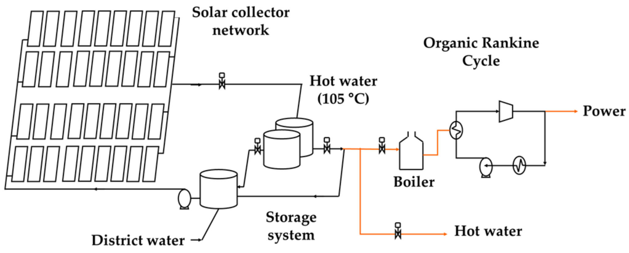
To supply the heat and power required by the process, two energy systems that operate independently were designed. In the design of the solar thermal installation to supply the heat load of the process, first the Pinch Analysis was used to reduce the auxiliary services, and simultaneously the network of solar collectors was designed to provide this requirement. Subsequently, an organic Rankine cycle was designed to provide the power of the plant where the thermal load of the evaporator is by means of low temperature solar thermal energy.

4.1. Solar Thermal Energy Integration Using Pinch Analysis

Using the concepts of Pinch Analysis, the integration of solar thermal energy was carried out for different Δ T m i n . Table 9 shows, for each Δ T m i n , the minimum hot utility requirement Q H , the minimum cold utility requirement Q C , the Pinch temperature T p i n c h , the area of the heat recovery network A H R N , the cost of the heat exchanger network C H R N , the costs of auxiliary services C A S , and the total annualised cost of the heat recovery network C T A   H R N .
It is important to highlight in Table 9, that there exists three Δ T m i n . where the minimum hot utility is small with respect to the rest of the values. The minimum hot utility is related with the heat recovery network and the auxiliary cost. These parameters are used to calculate kWhth solar, which has the lesser cost for a Δ T m i n = 7   ° C .
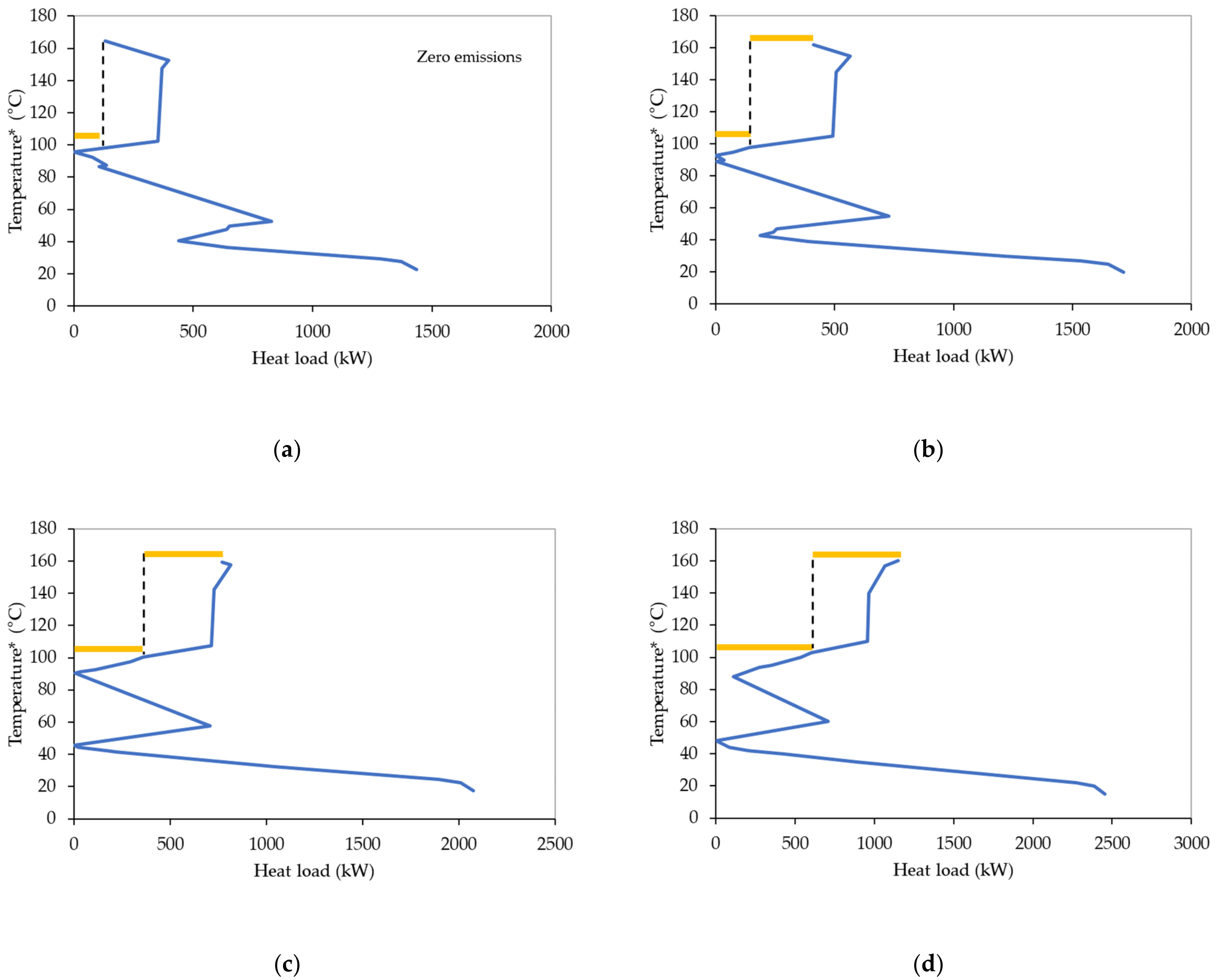
To identify the multiple utilities, the grand composite curve (GCC) is used. Figure 3 presents the GCC for different Δ T m i n ; an increase in the hot utility requirement is observed as Δ T m i n increases. To supply this thermal requirement through solar thermal energy, as the hot utility increases, the size of the solar collector network also increases. Low-temperature solar thermal energy is supplied at 105 °C. For Δ T m i n greater than 10 °C, the temperature levels to supply the hot utility are greater than 105 °C (therefore, the solar fraction f < 1 ), and it is not possible to reach those temperature levels with a network of low temperature collectors; however, with the steam obtained by burning bagasse, a window of possibility is highlighted, which are analysed.

4.2. Solar Thermal Installation Design

The design of the solar collector network is made for a temperature of 105 °C during a period of 3 h (11:15 a.m.–2:15 p.m.), with irradiance levels of the winter season. Solar thermal energy is stored to guarantee the supply of the thermal load and the temperature level required by the process. Table 10 shows the results obtained by evaluating different Δ T m i n , where Q H   S C N is the heat that can be supplied by a solar collector network at 105 °C for a period of 18 h.
Q H   A S and C A S correspond to the auxiliary heating service and its respective cost. To supply the thermal energy requirement of the process, it is necessary to have a storage system to guarantee the heat load at the target temperature level. The design of the solar collector network was based on values of irradiance data in the winter period in the city of Guanajuato. The dimensions of the components of the solar thermal installation and their costs are also shown, to estimate the total investment C T   S O L A R .
The Table 10 shows the Δ T m i n ; where the solar fraction is equal to one, it means the emissions to atmosphere are zero. The Δ T m i n = 5   ° C equation presents the minimum solar collector network and solar storage thermal cost. However, in the analysis there are other variables that must be considered, like the solar network area, limitations on installation area of the renewable system, and heat recovery network cost for the selection of Δ T m i n . There are many possibilities that could be the object of study that could be reached, using the result presented in Table 9 and Table 10.
Table 11 shows the energy savings, the payback of the solar thermal installation and the energy costs in USD per kWh for each Δ T m i n , which could be reached depending on the objective sought. The levelised cost of solar thermal energy L C O E t h   s o l a r corresponds to the solar thermal system, while the integrated system cost L C O E t h   i n t   s y s includes the solar thermal system, storage system and the heat recovery network system.
The L C O E t h   s o l a r does not present significant variations for different Δ T m i n , in contrast to the L C O E t h   i n t   s y s , due to the cost of the heat recovery network C H R N . 
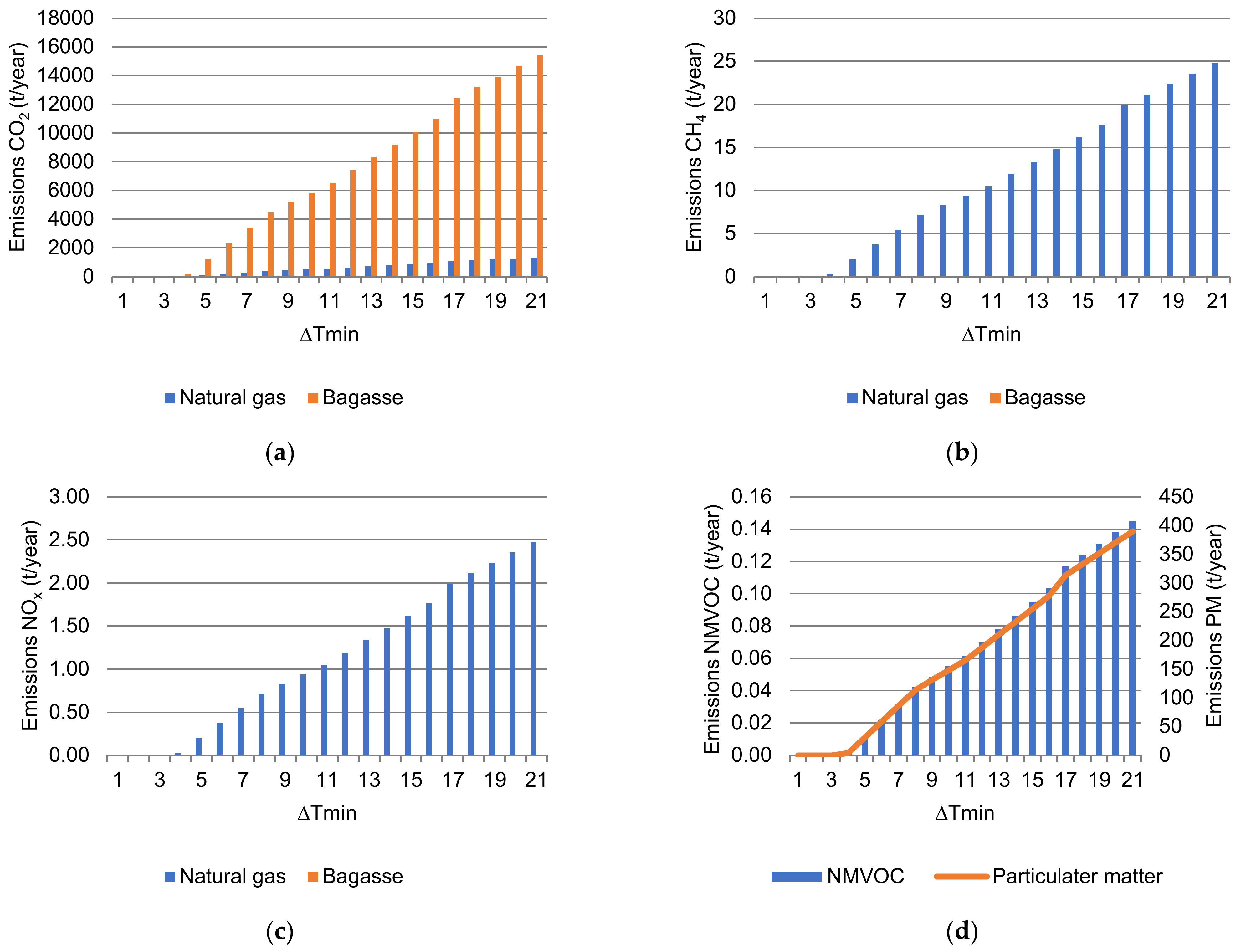
Figure 4 shows the results of the emissions generated by using natural gas and bagasse as fuel to produce the heat required by the process.
Emissions for different Δ T m i n are estimated for the combustion of natural gas and bagasse. For a Δ T m i n between 5–7 °C there are zero emissions, but the L C O E is higher. Analysing the Figure 4a, it could be observed that C O 2 emissions are much higher for bagasse compared to natural gas; for bagasse it represents 97% of total emissions. In Figure 4b,c, natural gas emits higher amounts of C H 4 and N O x into the atmosphere compared to bagasse. Figure 4d shows the emissions of NMVOC and PM for bagasse burning, and it is clearly observed that a large amount of solid particles are released into the environment. In all the graphs it is observed that at higher Δ T m i n the emissions grow; this due to the influence of the heat recovery network. For Δ T m i n between 5 and 7 °C, it is feasible to completely replace the use of fossil fuels for heat supply. When there are higher Δ T m i n , the auxiliary services increase, as do the emissions: this at a lower levelised energy cost of the integral system, L C O E t h   i n t   s y s .

4.3. Organic Rankine Cycle Results

The working fluid selected to be used in the power cycle to supply electrical energy to the process was the R290, due its thermodynamic properties and impact on the environment, (ODP = 0) and (GWP = 3). It is considered that to generate a power of 3.15 GW for 18 h, it is necessary to assume a total thermal load on the evaporator, and this is supplied by a solar thermal system (solar collector network and storage system) at 105 °C. The temperature in the evaporator is 90 °C for the design of the cycle and its components, and the condenser is considered to operate at atmospheric pressure. The design conditions of the ORC are shown in Table 12.
The results for different solar fractions are presented in Table 13. By varying the solar fraction (f), one part of total power will be supplied by the solar resource, and the other with the burning of biomass. The results show a lineal relationship that exists between the solar fraction with the size and cost of the components of the solar thermal system. However, the installation area of thermal storage A S S T , compared to the surface required by the solar collector network A S C N , is 116 times smaller. With the use of biomass, it is possible to reduce the cost, the number of collectors, and the installation area.
f Q H   Table 14 presents the levelised cost of energy of the ORC for different solar fractions, and also estimates the total cost of the annualised solar thermal installation. There are many important results that must be highlighted: simple payback time is almost the same for the solar fractions; savings for any solar fraction are big; cost associated with burning biomass increases significantly when the solar fraction decreases; and the cost of electrical power using solar thermal energy and biomass L C O E e l e is lower as the solar fraction increases.
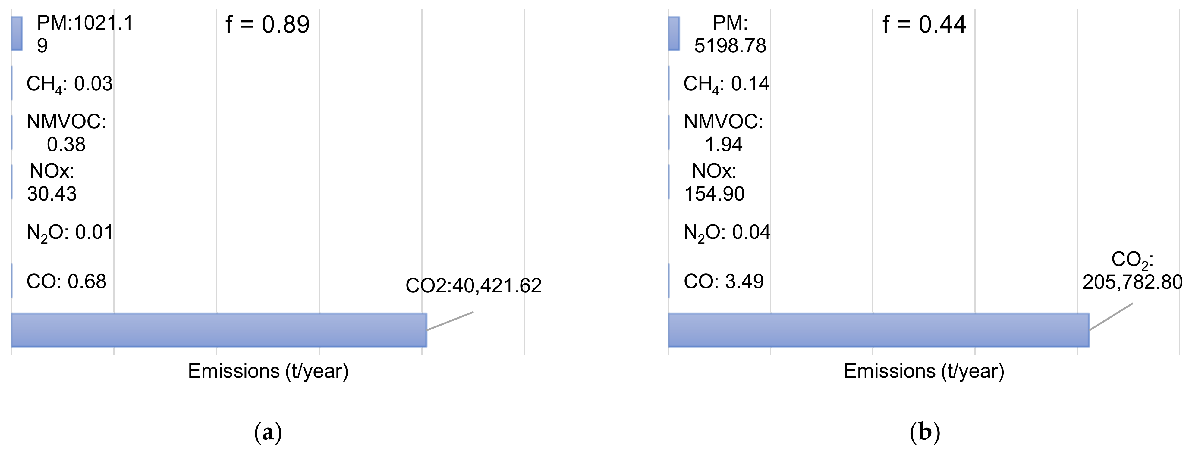
Emissions from burning sugarcane bagasse, for the power cycle, are shown in Figure 5 for two different solar fractions. For an f = 0.89, the amount of C O 2 emissions (40,421.62 t/year) and PM (1021.19 t/year) represents a serious impact on the environment and health due to the tons and the danger of the substances emitted.

4.4. Ways to Use Biomass and Solar Thermal Energy (Two Renewable Energies)

Case 1: Zero emissions. When the objective of the design is to completely replace the use of biomass, reducing to zero the emissions to supply the total heat and power to the process, the Δ T m i n   r e w selected is 7 °C, which has the lowest levelized cost of energy, 0.0636 USD/kWh. The required area of the solar collector field is 2813 m2. The levelised energy cost for L C O E e l e power production is 0.1392 USD/kWh, and the simple payback of the Rankine cycle is 20.9 years.
Case 2: Reduce NMVOC and PM emissions according to environmental regulations, or else, to minimize the impact on health. If the goal is to eliminate 10%, 30% or 50% of these emissions, the cost of electricity ( L C O E e l e ) and the simple payback are maintained, at an average of 0.1394 USD/kWh and 20.8 years, correspondingly. With this objective, 1.73 t/year of NMVOC and 4642 t/year of PM are no longer released into the atmosphere. The levelised cost of electrical energy L C O E e l e is 0.1394 USD/kWh for a solar fraction f = 0.50. Solar collector area was reduced by 48% with respect to the area for a solar fraction of one, with a simple payback time of 20.8 years.
Case 3: Reduce the size of the network collectors and storage system for power production. In this case, the design objective focuses on the availability of plant area for solar thermal installation. The solar collector field represents the largest required area of space compared to the storage surface, at a ratio of 116 times. If there is an available area of 10 hectares of surface, the solar fraction suggested to supply the power required by the process would be 0.22, with a total emission, E , of 294,091 t/year.
For the three cases, the heat process is supplied completely with solar thermal energy with a Δ T m i n of 7 °C.
The use of the renewable system, composed by solar thermal energy and biomass, is based on the preferential use of solar thermal energy, controlling the characteristic emissions originated by bagasse burning.
In the present work, three scenarios were studied; however, several more can be considered where a different objective set could be addressed, such as the limitations of installation area, project investment and payback time, and solar collector network area, among others.
The results achieved show that the relationship between the variables Δ T m i n , heat recovery network, solar collector network, storage tank, installation area, L C O E t h   s o l a r , L C O E e l e , emissions, project investment and payback time defines the final design of the renewable energy system composed by solar thermal energy and biomass.
It is sought that the Δ T m i n reduces the auxiliary heating service, and thus eliminates the largest amount of emissions considering the profitability of the system. It is noted that the cost of solar thermal energy ( L C O E t h   s o l a r ) is in a range of 0.0649–0.0621 USD/kWh; however, when adding the cost of the heat recovery network, this value is increased by 0.7363–0.4926 USD/kWh, that is, the cost of the integrated system is doubled due to cost to the heat recovery network. In power production, the average levelised cost of energy ( L C O E e l e ) is 0.1394 USD/kWh, which remains practically constant when the solar fraction varies. However, the solar collectors network area for power production changes drastically with the solar fraction. In the same way, when solar fraction decreases, with a consequent rise in biomass burning, the C O 2 tons are 12 times the amount generated by the burning of natural gas. Reduction of emissions should be a design target in itself.
In the study by Tilahun et al., 2020, [33] regarding the cogeneration of heat and electricity, they proposed a hybrid solar-biomass energy system. They performed an optimisation with the objective of maximising the solar fraction with the lowest investment cost, obtaining L C O E = 0.094 USD/kWh for f = 0.235. A Prosopis juliflora tree was used as biomass, because it is abundant in the study location. However, the burning of wood did not solve the long-term environmental impact. In the present work, with a L C O E e l e = 0.1392 USD/kWh (f = 1), it is feasible to eliminate the emissions.

5. Conclusions

The proposed approach enabled control of the generated emissions, putting special attention on the dangerous emissions produced by the burning of biomass. It is not possible to use biomass burning as a backup system, but rather as a complement where the operator has control over the amount of emissions generated and the consequent impact on the environment.
Based on the results in one of the analysed cases, it is feasible to supply the full thermal load of the process, thus eliminating the burning of bagasse and the generation of dangerous emissions to atmosphere.
In power production, the area of the solar collector network can be reduced by 68% by decreasing the burning of bagasse by 30%, keeping the energy cost and recovery time constant (0.1395 USD/kWh, 20.8 years).
Regarding power production, there is an area of opportunity, because the technology efficiency must be improved to reduce the large areas of solar collectors (32 hectares) that are required. This makes evident the convenience of using biomass, as long as it is controlling emissions.
The design method can be adjusted for other renewable technologies and globally to assess the environmental impact and economic cost. Regarding the existing control from the design, and the generation of emissions into the atmosphere, it can be adjusted according to the regulations of each country or region.
In any of the scenarios proposed, the cost of electrical energy and thermal energy is competitive compared to the global market.

Author Contributions

Conceptualization, G.M.-R. and J.-C.B.; methodology, A.L.F.-S.; software, A.L.F.-S.; validation, G.M.-R.; formal analysis, G.M.-R. and R.G.-G.; investigation, G.M.-R., J.-C.B., A.L.F.-S. and R.G.-G.; resources, G.M.-R.; data curation, A.L.F.-S.; writing—original draft preparation, G.M.-R.; writing—review and editing, G.M.-R. and J.-C.B.; visualization, G.M.-R.; supervision, G.M.-R.; project administration, G.M.-R.; funding acquisition, G.M.-R. All authors have read and agreed to the published version of the manuscript.

Funding

This research received no external funding. The APC was funded by ASPAAUG, Universidad de Sonora and University of Guanajuato.

Institutional Review Board Statement

Not applicable.

Informed Consent Statement

Not applicable.

Data Availability Statement

Not applicable.

Acknowledgments

To Evangelina Sánchez-García for editing support.

Conflicts of Interest

The authors declare no conflict of interest.

References

  1. Martínez-Rodríguez, G.; Fuentes-Silva, A.L.; Lizárraga-Morazán, J.R.; Picón-Núñez, M. Incorporating the Concept of Flexible Operation in the Design of Solar Collector Fields for Industrial Applications. Energies 2019, 12, 570. [Google Scholar] [CrossRef] [Green Version]
  2. Valderrama, C.; Quintero, V.M.; Kafarov, V. Energy and water optimization of an integrated bioethanol production process from molasses and sugarcane bagasse: A Colombian case. Fuel 2020, 260, 116314. [Google Scholar] [CrossRef]
  3. Da Silva, P.H.; Lodi, A.; Aoki, A.C.; Modesto, M. Energy, exergetic and economic analyses of a combined solar-biomass-ORC cooling cogeneration systems for a Brazilian small plant. Renew. Energy 2020, 157, 1131–1147. [Google Scholar] [CrossRef]
  4. Tsimpoukis, D.; Syngounas, E.; Bellos, E.; Koukou, M.; Tzivanidis, C.; Anagnostatos, S.; Vrachopoulos, M.G. Investigation of energy and finncial performance of a novel CO2 supercritical solar-biomass trigeneration system for operation in the climate of Athens. Energy Convers. Manag. 2021, 245, 114583. [Google Scholar] [CrossRef]
  5. Chagger, H.K.; Kendall, A.; McDonald, A.; Pourkashanian, M.; Williams, A. Formation of dioxins and other semi-volatile organic compounds in biomass combustion. Appl. Energy 1998, 60, 101–114. [Google Scholar] [CrossRef]
  6. Ren, Y.; Shen, G.; Shen, H.; Zhong, Q.; Xu, H.; Meng, W.; Zhang, W.; Yu, X.; Yun, X.; Luo, Z.; et al. Contributions of biomass burning to global and regional SO2 emissions. Atmos. Res. 2021, 260, 105709. [Google Scholar] [CrossRef]
  7. Malico, I.; Pereira, R.; Gonçalve, A.; Sousa, A. Current status and future perspectives for energy production from solid biomass in the European industry. Renew. Sustain. Energy Rev. 2019, 112, 960–977. [Google Scholar] [CrossRef]
  8. Bertazzi, P.A.; Consonni, D.; Bachetti, S.; Rubagotti, M.; Baccarelli, A.; Zocchetti, C.; Pesatori, A.C. Health effects of dioxin Exposure: A 20-Year mortality study. Am. J. Epidemiol. 2001, 153, 1031–1044. [Google Scholar] [CrossRef]
  9. Cheruiyot, N.K.; Lee, W.J.; Yan, P.; Mwangi, J.K.; Wang, L.C.; Gao, X.; Lin, N.H.; Chang-Chien, G.P. An overview of PCDD/F inventories and emission factors from stationary and mobile sources: What we know and what is missing. Aerosol Air Qual. Res. 2016, 16, 2965–2988. [Google Scholar] [CrossRef] [Green Version]
  10. Schecter, A.; Birnbaum, L.; Ryan, J.J.; Constable, J.D. Dioxins: An overview. Environ. Res. 2006, 101, 419–428. [Google Scholar] [CrossRef]
  11. Demirbas, M.F. Emissions of polychlorinated dibenzo-p-dioxins and dibenzofurans from biomass combustion and solid waste incineration. J. Energy Sources Part A Recovery Util. Environ. Eff. 2007, 29, 1041–1047. [Google Scholar] [CrossRef]
  12. Yu, L.; Mai, B.; Meng, X.; Bi, X.; Sheng, G.; Fu, J.; Peng, P.A. Particle-bound polychlorinated dibenzo-p-dioxins and dibenzofurans in the atmosphere of Guangzhou, China. Atmos. Environ. 2006, 40, 96–108. [Google Scholar] [CrossRef]
  13. Wang, G.; Zhang, R.; Gomez, M.E.; Yang, L.; Zamora, M.L.; Hu, M.; Lin, Y.; Peng, J.; Guo, S.; Meng, J.; et al. Persistent sulfate formation from London fog to Chinese haze. Proc. Natl. Acad. Sci. USA 2016, 113, 13630–13635. [Google Scholar] [CrossRef] [PubMed] [Green Version]
  14. Zhong, Q.; Shen, H.; Yun, X.; Chen, Y.; Ren, Y.; Xu, H.; Shen, G.; Du, W.; Meng, J.; Li, W.; et al. Global sulfur dioxide emissions and the driving forces. Environ. Sci. Technol. 2020, 54, 6508–6517. [Google Scholar] [CrossRef] [PubMed]
  15. Sánchez de la Campa, A.M.; Salvador, P.; Fernandez-Camacho, R.; Artinano, B.; Coz, E.; Márquez, G.; Sánchez-Rodas, D.; De la Rosa, J. Characterization of biomass burning from olive grove areas: A major source of organic aerosol in PM10 of Southwest Europe. Atmos. Res. 2018, 199, 1–13. [Google Scholar] [CrossRef]
  16. Wang, S.X.; Zhao, B.; Cai, S.Y.; Klimont, Z.; Nielsen, C.P.; Morikawa, T.; Woo, J.H.; Kim, Y.; Fu, X.; Xu, J.Y.; et al. Emission trends and mitigation options for air pollutants in East Asia. Atmos. Chem. Phys. 2014, 14, 6571–6603. [Google Scholar] [CrossRef] [Green Version]
  17. OCDE-FAO Perspectivas Agrícolas 2020–2029. 2018. Available online: https://www.oecd-ilibrary.org/ (accessed on 15 February 2022).
  18. Nullis, C.; Oficina de Comunicación y de Relaciones Públicas de la OMM. Informe Especial Sobre el Calentamiento Global de 1.5 °C. 2018. Available online: https://public.wmo.int/es/resources/bulletin/el-ipcc-publica-el-informe-especial-sobre-el-calentamiento-global-de-15-%C2%B0c (accessed on 15 February 2022).
  19. Algieri, A.; Morrone, P. Comparative energetic analysis of high temperature subcritical and transcritical Organic Rankine Cycle (ORC). Appl. Thermal. Eng. 2012, 36, 236–244. [Google Scholar] [CrossRef]
  20. Martínez-Rodríguez, G.; Fuentes-Silva, A.L.; Baltazar, J.-C. Simultaneous Production of Solar Thermal Heat and Power for Industrial Applications. Chem. Eng. Trans. 2021, 88, 505–510. [Google Scholar] [CrossRef]
  21. Renewables 2018, Global Status Report. Available online: https://www.ren21.net/reports/global-status-report/ (accessed on 15 February 2022).
  22. Lizárraga-Morazán, J.R.; Martínez-Rodríguez, G.; Fuentes-Silva, A.L.; Picón-Núnez, M. Selection of solar collector network design for industrial applications subject to economic and operation criteria. Energy Environ. 2021, 32, 1504–1523. [Google Scholar] [CrossRef]
  23. Facão, J.; Oliveira, A.C. Analysis of energetic, design and operational criteria when choosing and adequate working fluid for small ORC system. In Proceedings of the ASME 2009 International Mechanical Engineering Congress & Exposition, IMECE2009-12420, Lake Buena Vista, FL, USA, 13–19 November 2009. [Google Scholar]
  24. Mago, P.; Chamra, L.M.; Srinivasan, K.; Somayaji, C. An examination of regenerative organic Rankine cycles using dry fluids. Appl. Therm. Eng. 2008, 28, 998–1007. [Google Scholar] [CrossRef]
  25. Sinnott, R.K.; Towler, G. Chemical Engineering Design Principles, Practice and Economics of Plant and Process Design, 1st ed.; Butterworth-Heinemann of Elsevier: Boston, MA, USA, 2008. [Google Scholar]
  26. Valencia, G.; Cárdenas, J.; Duarte, J. Exergy, Economic, and Life-Cycle Assessment of ORC System for Waste Heat Recovery in a Natural Gas Internal Combustion Engine. Resources 2020, 9, 2. [Google Scholar] [CrossRef] [Green Version]
  27. Gil-Unday, Z. Estudio del Impacto Ambiental del uso del Bagazo como Fuente de Energía en Centrales Azucareros en Cuba. Estudio de Caso “Melanio Hernández”. Ph.D. Thesis, Universitat de Girona, Girona, Spain, 2005. Available online: https://dialnet.unirioja.es/institucion/406/buscar/tesis?querysDismax.DOCUMENTAL_TODO=melanio (accessed on 25 May 2021).
  28. GHG Emission Factors Hub US EPA. Available online: https://www.emissionfactors.com/?gclid=EAIaIQobChMItOf51uWh9gIVwTytBh1FNApBEAAYASAAEgKgpvD_BwE (accessed on 10 April 2021).
  29. Report Global Energy Transformation IRENA. Available online: https://www.irena.org/-/media/Files/IRENA/Agency/Publication/2018/Apr/IRENA_Report_GET_2018.pdf (accessed on 15 February 2022).
  30. Wahed, A.; Bieri, M.; Kui, T.K.; Reindl, T. Levelized Cost of Solar Thermal System for Process Heating Applications in the Tropics. In Transition towards 100% Renewable Energy, 1st ed.; Sayigh, A., Ed.; Springer: Cham, Switzerland, 2018; pp. 441–450. [Google Scholar] [CrossRef]
  31. Energybot Texas Electricity Prices. Available online: https://energybot.com/electricity-rates/texas/ (accessed on 15 February 2022).
  32. Global Petrol Prices. Available online: https://www.globalpetrolprices.com/gasoline_prices/ (accessed on 15 February 2022).
  33. Tilahun, F.B.; Bhandari, R.; Mamo, M. Design optimization of a hybrid solar-biomass plant to sustainably supply energy to industry: Methodology and case study. Energy 2021, 220, 119736. [Google Scholar] [CrossRef]
Figure 1. Production of 1G and 2G bioethanol from sugarcane.
Energies 15 02338 g001
Figure 2. Basic scheme of the proposed organic Rankine cycle.
Energies 15 02338 g002
Figure 3. Grand composite curves for different Δ T m i n that show how it is possible to supply the total heat process in the 1G and 2G bioethanol production described lines above. (a) Δ T m i n of 5 °C; (b) Δ T m i n of 10 °C; (c) Δ T m i n of 15 °C; (d) Δ T m i n of 20 °C.
Energies 15 02338 g003
Figure 4. Variation of emissions for different Δ T m i n . (a) Carbon dioxide, C O 2 , emissions; (b) Methane, C H 4 , emissions; (c) Nitrogen oxides, N O x , emissions; (d) Non-methane volatile organic compounds, NMVOC, and particulate matters emissions from bagasse.
Energies 15 02338 g004
Figure 5. Estimated emissions for different solar fractions. (a) f = 0.89; (b) f = 0.44.
Energies 15 02338 g005
Table 1. Calorific value of sugarcane bagasse in kJ/kg.
Calorific Value (kJ/kg)
Bagasse (wet basis)8477.4
Bagasse (dry)18,096.7
Table 2. 1G and 2G bioethanol process stream data.
StreamDescriptionTin (°C)Tout (°C)CP (kW/°C)h (kW/m2 °C)
H1Neutralisation 1167.050.022.192.0
H2Neutralisation 252.025.07.632.0
H3Neutralisation 352.030.044.652.0
H4Distillation 198.032.048.362.0
H5Distillation 2150.025.05.432.0
C1Extraction juice25.090.014.403.0
C2Clarification 134.085.040.343.0
C3Clarification 284.0100.050.033.0
C4Separation 138.050.080.143.0
C5Separation 293.0150.027.973.0
Table 3. Cost functions for the components of the Rankine cycle in USD.
Component/EquipmentCost Functions
Turbine ,   C t u r C t u r = 10 2.6259 + 1.4389 l o g W t u r b 0.1776 l o g W t u r b 2  
Pump ,   C p u m p C p u m p = 549.13 W p u m p 0.71 1 + 0.2 1 η p u m p
Heat   exchangers   ( evaporator   and   condenser ) ,   C h x C h x = 516.621 A + 268.45
Table 4. Emissions index.
Indext/GWhkg/kWh
C O 0.0363.6 × 10−5
C O 2 2125.62.13
N 2 O 4.3 × 10−44.30 × 10−7
N O x 1.61.60 × 10−3
S O x 00
NMVOC0.022.00 × 10−5
C H 4 1.4 × 10−31.40 × 10−6
Particulate matters53.75.37 × 10−2
Table 5. Emission factors for greenhouse gas inventories.
FactorNatural GasBagasse
kg/MMBTUkg/MMBTUkg/kWhkg/MMBTUkg/kWh
C O 2 53.060.18195.50.326
C H 4 1.0 × 10−33.410 × 10−61.9 × 10−36.48 × 10−6
N 2 O .1.0 × 10−43.410 × 14.2 × 10−41.43 × 10−6
Table 6. Cost of energy services.
Indext/GWh
Steam/heating16.9102 USD/MMBTU
Cooling water9.0852 USD/MMBTU
Electricity0.0838 USD/kWh (Texas, 2022) [31]
Table 7. Fuel prices reported in 2021.
Natural Gas0.0480 USD/kWh (word average, 2021) [32]
0.052 USD/kWh (Germany, 2021) [32]
Sugarcane Bagasse (Briquette)145 USD/t [33]
Table 8. Emissions from biomass burning of the process under study.
Fuel C O 2   ( t / Year ) C O   ( t / Year ) N 2 O   ( t / Year ) N O x   ( t / Year ) S O x   ( t / Year ) NMVOC (t/Year) C H 4   ( t / Year ) Particulate Matters (t/Year)
Bagasse [27]378,711.536.410.0766285.06700.00003.56330.24949567.56
Natural gas [28]32,257-60.79---607.93-
Table 9. Minimum energy requirements and costs of the heat recovery network for different Δ T m i n .
Δ T m i n   ( ° C ) Q H   ( kW ) Q C   ( kW ) T p i n c h   ( ° C ) A H R N   ( m 2 ) C H R N   ( USD ) C A S   ( USD / Year ) C T A   H R N   ( USD / Year )
131143695.55322,346,716337,514619,044
6181148695.04962,224,894366,270633,185
7231153694.54662,123,404395,026649,765
10410171593.03891,899,159497,847725,685
15769203845.52901,582,982696,776886,683
201149245448.02301,363,688922,3651,085,964
251528283450.52001,253,5471,140,7231,291,108
Table 10. Results of the design of the solar thermal installation for different Δ T m i n .
Δ T m i n   ( ° C ) Q H   S C N   ( kW ) Q H   A S   ( kW ) f C A S   ( USD / Year ) N C A C   ( m 2 ) C S C N   ( USD ) V S S T   ( m 3 ) C S S T   ( USD ) C T   S O L A R   ( USD )
513101288,5228701592531,5102457,075588,586
618101298,57212182229744,1153467,992812,107
723101308,62215372813939,0024377,1921,016,194
102421680.59407,51015952919974,4364578,8011,053,236
152944740.38586,776194335561,187,0405488,1091,275,149
203527970.31790,773234942991,435,0786698,3571,533,435
2540811200.27988,128269749361,647,68275106,7221,754,404
Table 11. Design costs of the solar thermal installation for different Δ T m i n .
Δ T m i n   ( ° C ) Savings (USD/Year)Payback Solar Thermal (Year) L C O E t h   s o l a r   ( USD / kWh ) L C O E t h   i n t   s y s   ( USD / kWh )
525,89722.70.06490.7363
635,78522.70.06480.5468
745,75222.20.06360.4398
1047,75222.10.06300.4688
1558,14621.90.06270.4701
2069,55922.00.06300.4815
2580,66121.80.06210.4926
Table 12. ORC design conditions data.
T 3 (°C) P 3 (kPa) T 4   ( ° C ) P 4   ( kPa ) T 1   ( ° C ) P 1   ( kPa ) T 2   ( ° C ) P 2   ( kPa ) η O R C
9024022510032510032624020.129
Table 13. Costs of the solar thermal installation to supply the thermal load of an ORC by varying the solar fraction.
f Q H   (kW) N C A C   ( m 2 ) C S C N   ( USD ) V S S T   ( m 3 ) C S S T   ( USD ) A S S T   ( m 2 ) C T   S O L A R (USD)
10176,030322,135107,542,27349171,707,0062788109,249,278
0.892935156,658286,68495,707,30843761,574,477248197,281,785
0.785869137,286251,23383,872,34238351,436,925217485,309,268
0.678804117,943215,83672,055,09432941,293,622186873,348,716
0.5611,73998,571180,38560,220,12927531,142,821156161,362,950
0.4414,94077,459141,75047,322,1432164967,872122748,290,015
0.3317,87558,087106,29935,487,1781622794,18192036,281,359
0.2220,80938,74470,90223,669,9301082602,08861424,272,018
0.1123,74419,37235,45111,834,965541376,76830712,211,733
Table 14. Levelised cost of energy for different solar fractions.
f C T A   S O L A R   ( USD / Year ) Fuel Cost (USD)Savings (USD/Year)Payback (Year) L C O E e l e   ( USD / kWh )
110,234,33905,272,77620.70.1392
0.899,113,239580,0054,692,77120.70.1392
0.787,991,6681,160,0114,112,76520.70.1393
0.676,871,2181,740,0163,532,76020.80.1393
0.565,748,4062,320,0212,952,75420.80.1394
0.444,523,7502,952,7552,320,02120.80.1395
0.333,398,7933,532,7601,740,01620.90.1396
0.222,273,7734,112,7651,160,01020.90.1398
0.111,143,9804,692,771580,00521.10.1402
Publisher’s Note: MDPI stays neutral with regard to jurisdictional claims in published maps and institutional affiliations.

