LPSRS: Low-Power Multi-Hop Synchronization Based on Reference Node Scheduling for Internet of Things

Abstract

Time synchronization is one of the most fundamental problems on the internet of things (IoT). The IoT requires low power and an efficient synchronization protocol to minimize power consumption and conserve battery power. This paper introduces an efficient method for time synchronization in the IoT called low-power multi-hop synchronization (LPSRS). It employs a reference node scheduling mechanism to avoid packet collisions and minimize the communication overhead, which has a big impact on power consumption. The performance of LPSRS has been evaluated and compared to previous synchronization methods, HRTS and R-Sync, via real hardware networks and simulations. The results show that LPSRS achieves a better performance in terms of power consumption (transmitted messages). In particular, for a large network of 450 nodes, LPSRS reduced the total number of transmitted messages by 53% and 49% compared to HRTS and R-Sync, respectively.

1. Introduction

The internet of things (IoT) plays a remarkable role and makes the quality of our life efficient. It has been extensively studied and developed in recent years. The IoT is generally applied to many areas, including healthcare, transportation, wireless networks, and industry. The wireless sensor nodes (WSNs) are one of the prime parts of IoT applications. They face many challenges to exchange information and cooperate in wireless applications [1,2]. One of these challenges is power consumption. Generally, sensor nodes are frequently battery-powered in most IoT applications. To reduce the battery power consumption and increase the battery lifetime, sensor nodes switch between active and sleep modes. To wake up sensor nodes at a predetermined time, most of them require time synchronization [3,4]. Sensor nodes, as a result, require trust and reliable synchronization [5].

Sensor nodes are frequently equipped with a relatively inexpensive hardware clock oscillator [6]. As a result, reliable time synchronization for such sensor nodes is more difficult [7]. Time synchronization of such wireless networks with such sensor nodes cannot be well-preserved for an extended period of time unless an accurate synchronization technique is performed on a constant schedule [7]. In time division multiple access (TDMA) networks, a node’s wake-up time might be completely erroneous due to a lack of synchronization, resulting in severe network connectivity failure. Therefore, time synchronization is considered an essential and important aspect of the sensor nodes’ operations. It offers a common reference time for all sensor nodes in the entire network [8,9].

Generally, to keep the whole network well synchronized and to minimize time offsets caused by clock drift, all sensor nodes should require continuously exchanging timing messages [10]. Exchanging timing messages between the nodes is commonly utilized for time synchronization in sensor node networks. Since the transmission of messages usually accounts for most of the power consumption, frequent synchronization significantly increases power consumption [5,8]. Generally, time synchronization in IoT sensor nodes has two main problems: (1) communication overhead, which can be represented by the number of transmitted messages, and (2) accuracy. Both of these problems lead to a significant rise in power consumption [4,9].

Several protocols for sensor node synchronization have been developed. These protocols have been developed to synchronize all nodes in large networks [11]. The majority of these protocols aimed to enhance synchronization accuracy at the expense of higher communication overhead [2,4]. On the other hand, there are a few proposed protocols that are interested in reducing power consumption by reducing overhead connections [4,9]. Moreover, due to frequent collisions, these protocols suffer from message loss. Collisions have an effect on power usage and may result in synchronization failure [5,7].

All of these issues and problems motivate us to establish the low-power synchronization based on reference node scheduling (LPSRS) for IoT. It can save an amount of energy by reducing the number of timing messages sent between sensor nodes. Furthermore, LPSRS implements a technique that fully and completely prevents node collisions during the time synchronization process. According to experimental results and simulations, the performance of LPSRS has been extensively investigated compared to HRTS [12] and R-Sync [9]. The results demonstrate that LPSRS reduces the total number of transmitted messages by 53%, 49%, and 13% compared to HRTS, R-Sync, and FADS, respectively, and, thus, LPSRS can minimize the power consumption for time synchronization in the IoT.

The remainder of the paper is structured as follows: We address the related work in Section 2, while the preliminaries and system model of LPSRS are described in Section 3. Section 4 elaborates on the operations of LPSRS. Section 5 presents the experimental and simulation setup and discusses the results. This is followed by the simulation results. Finally, in Section 6, we conclude our work.

2. Related Work

Sensor nodes’ time synchronization has been extensively researched over many decades. Many methods for clock synchronization have been proposed in the literature, all of which seek to reduce power consumption by improving accuracy and lowering communication overhead.

The flooding time synchronization protocol (FTSP) [13] pursues to minimize the error of synchronization by using the least square linear regression (LSLR) to compensate for the clock drift. Lenzen et al. have reported that the global synchronization error of FTSP rises exponentially with the size of the network [14,15]. They, then, propose a scalable technique called PulseSync, which can quickly flood the timing information all over the network [14]. Yildirim et al. indicated possible drawbacks of quick flooding and suggested a clock speed agreement algorithm. He proposed flooding with clock speed agreement (FCSA) [6] and an adaptive value tracking synchronization (AVTS) [16]. FCSA and AVTS, however, need many messages which increase the chance of collision and result in excessive power consumption [11].

The reference broadcast synchronization (RBS) [17] is typically a receiver-to-receiver protocol (RRP). By excluding the transmitter’s delays from the offset computations, it improves the accuracy of the time offset estimate. In RBS, however, it sends a large number of messages in each cycle of the synchronization [7]. This leads to two different problems: a high chance of collision and excessive power consumption. Gong et al. developed the energy-efficient coefficient exchange synchronization protocol (CESP) to solve these issues [18]. Compared to RBS, it makes use of the synchronization coefficient to relatively reduce communication costs. CESP, on the other hand, is based on a stationary reference node and, thus, absorbs a lot of energy [9].

In [19], the timing-sync protocol for sensor networks (TPSN) was introduced. Although TPSN has good scalability, it requires regular resynchronization [20]. Furthermore, because of the enormous number of message exchanges required by TPSN, it consumes a lot of power [7]. Hierarchy reference broadcast synchronization (HRTS) [12] contains three stages that are repeated at every hierarchical level all over a multi-hop network. In HRTS, it is presumed that each node is aware of its adjacent neighbors. Despite being a scalable and lightweight protocol, HRTS has two drawbacks: high communication costs and excessive collisions [11].

M. Elsharief et al. introduced a synchronization technique called FADS [7]. FADS uses a scheduling technique to organize message transmission among sensor nodes, which reduces the number of collisions. FADS reduces latency by speeding up the scheduling process. During the scheduling process, FADS, however, requires a relatively large number of message transmissions, which consumes a lot of power [21].

The robust time synchronization (R-sync) for the industrial internet of things (IIOT) was also introduced in [9]. It focuses on locating and reconnecting the network’s isolated nodes that have lost synchronization [22]. Despite the reality that R-sync needs fewer messages than TPSN, it lacks a collision avoidance technique.

In contrast to previous approaches, average time synchronization (ATS) [23] is a fully distributed method. To calibrate its compensation parameters, ATS employs a cascade of two consensus methods, and it allows nodes to converge to a steady-state virtual clock [5]. However, ATS suffers from frequent collisions, which might result in synchronization method failure [7]. To address the aforementioned shortcoming of ATS, the selective average time synchronization (SATS) [24] protocol has been suggested. It employs a dynamic programming method to increase the speed and accuracy of convergence in sparse WSNs. It achieves faster convergence than other protocols (ATSP [25] and CCS [26]). SATS, on the other hand, increases the number of transmitted messages since each node in SATS must forward every received message [27]. Based on ATS, the multi-hop average consensus time synchronization protocol (MACTS) [28] has been proposed. To improve the algebraic connectedness of the large-scale network, it leverages the notion of virtual communication linkages among multi-hop nodes. MACTS, like SATS, must send additional messages throughout the synchronization process. Message forwarding in large-scale networks, such as MACTS, can be delayed due to congestion among surrounding nodes [27].

The notion of density-based scheduling was introduced in [29], which can minimize overhead by reducing the number of reference nodes. It may, nevertheless, experience reception failure as a result of frequent packet collisions. Furthermore, it frequently suffers from coverage issues since it does not ensure the synchronization of some nodes that are not within the wireless range of any chosen reference nodes [7]. In [21], the low-power scheduling for synchronization protocol (LPSS) was introduced. It is a free collision m method. LPSS reduces the number of messages and accelerates the scheduling process. It, however, does not provide a synchronization scheme. In [30], Geo-TimeSyc was proposed. Geo-TimeSyc partitions the network into separated regions to avoid concurrent transmission of neighboring nodes. It reduces the probability of collisions [31]. As Geo-TimeSyc is implemented with RBS, it needs a large number of message exchanges. Recently, we proposed an energy-efficient synchronization technique called EERS [4]. It is a free collision protocol. Although ERRS substantially reduces energy consumption, it is only suitable for networks in which the nodes’ locations are known.

From a thorough analysis of prior studies, we found that most of the prior techniques suffer from a serious problem of high power consumption. Hence, it is highly challenging to provide low-power synchronization. This problem motivates us to find a new technique to resolve it. Our approach, LPSRS, uses a scheduling method of [21] that tries to cover all nodes with as few reference nodes as possible. Then, it applies the synchronization scheme to synchronize all nodes in the entire network. LPSRS can save a large amount of energy by minimizing the usage of messages were sent and preventing collisions. As a result, LPSRS’s contributions can be summarized in the following points:

(1)

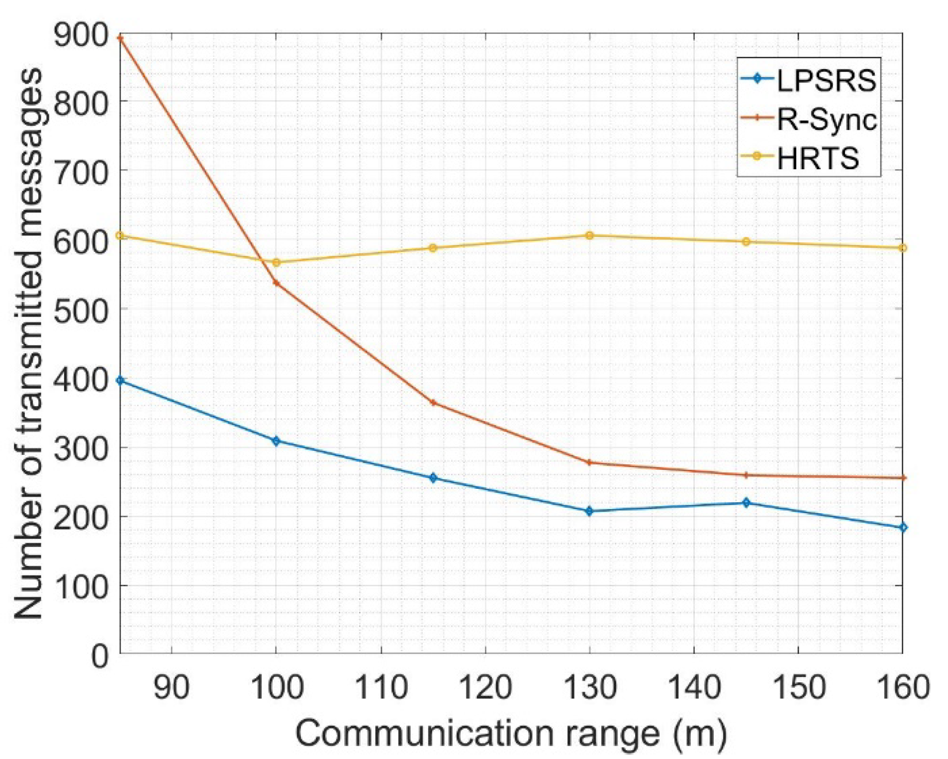
LPSRS substantially reduces transmission overhead (number of transmitted messages), thereby lowering power consumption.

(2)

LPSRS utilizes a scheduling approach to address the collision issue, which can reduce power consumption.

(3)

LPSRS is constructed into a real wireless sensor network with different configurations and an extensive simulation with large-scale networks.

3. Preliminaries

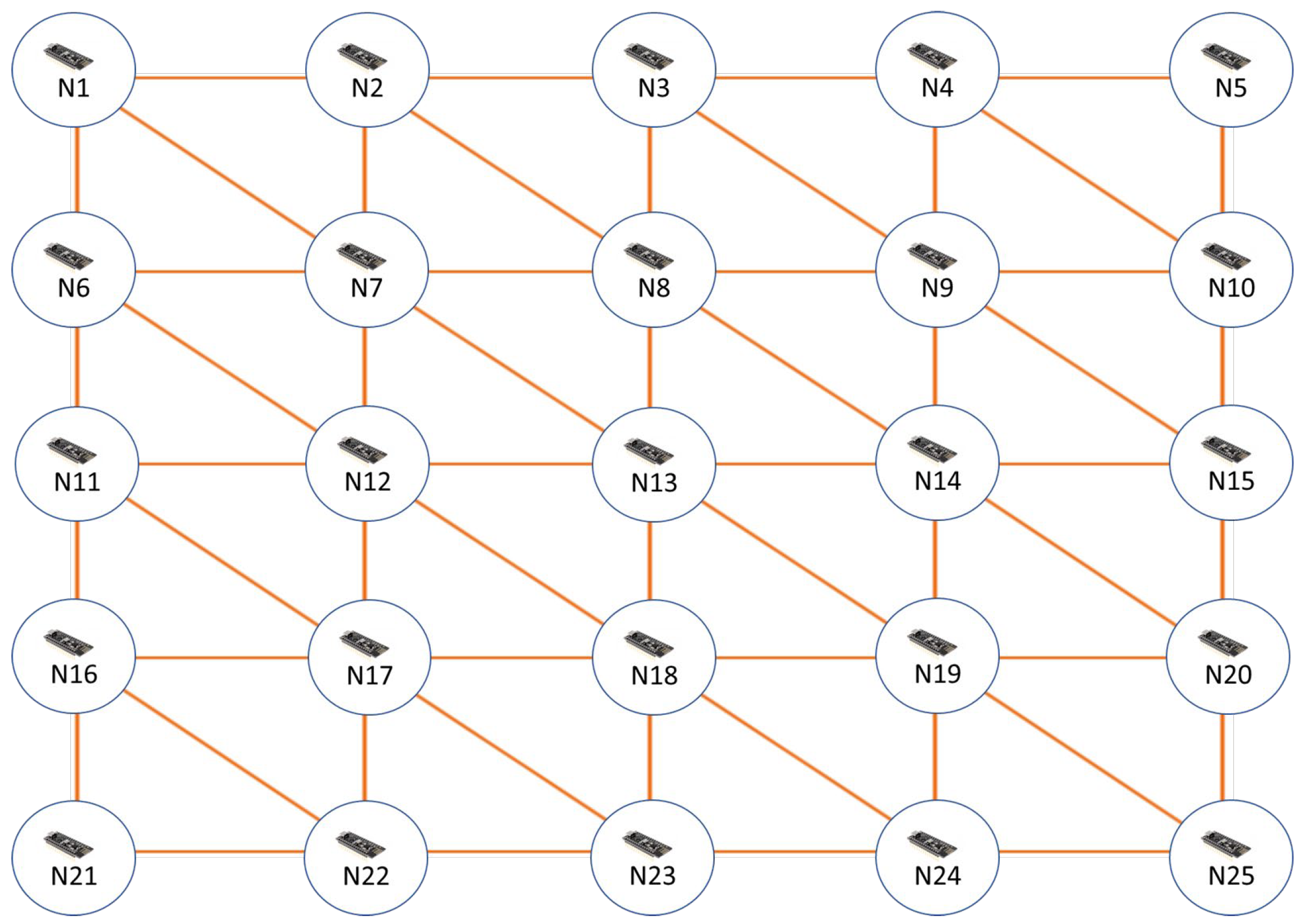
3.1. System Model

A sensor network is designed as a graph $G=\left(V,E\right)$ consisting of a set of vertices, $V=\left\{1,2,\dots .,\dots ,N\right\},$ representing the sensor nodes and a set of edges, $E\subseteq V\times V,$ representing the two-way communication links among the nodes. We refer to the nodes located within the wireless range of a node $i\in V$ as the neighbors of node $i$. These neighbor nodes of node $i$ are denoted by $\mathbb{V}\left(i\right)=\{j\in V|\left\{i,j\right\}\in E\}$. Each node in this article has its own unique ID number $\left(\ge 1\right)$ as well as a hardware clock. Simply for the purpose of clarity, we assume that the network is fixed and the communication between the nodes is fully reliable. Besides, we also presume that each node is supplied with an omnidirectional antenna and has a steady wireless range of an $r$ meter radius. Moreover, we assume that the sink node recognizes all neighbor nodes of every node in the network [21].

3.2. Message Format

LPSRS utilizes two types of messages: the first one is used for the scheduling process, while the other one is used for the synchronization process. The first scheduling message includes the following fields:

(1)

DestAddr: a destination address of the message.

(2)

MesN: a number of split messages of the scheduling message. Its default value is 1.

(3)

SrcID: a unique identifier of the sender.

(4)

Type: the type of message is Sch (i.e., scheduling message).

(5)

RefNodes: list of reference nodes.

(6)

SchSlots: list of scheduled time slots.

(7)

SeqN: sequence number of the scheduling messages. Its default value is 0.

Meanwhile, the synchronization message has the following fields:

(1)

DestAddr: the destination address of the message.

(2)

SrcID: the unique identifier of the sender.

(3)

SID: specified reference node. Its default value is −1.

(4)

Type: the type of messages, including $Sync1$, $Sync2$, and $Sync3$.

(5)

SeqN: sequence number of the synchronization messages. Its default value is 0.

(6)

RT: the timestamp at the moment of receiving $Sync1$. Its default value is −1.

(7)

TS: the timestamp at the moment of sending $Sync2$. Its default value is −1.

(8)

RefT: the timestamp of the reference time when receiving $Sync3$. Its default value is −1.

(9)

OF: the offset value when sending $Sync3$. Its default value is 0.

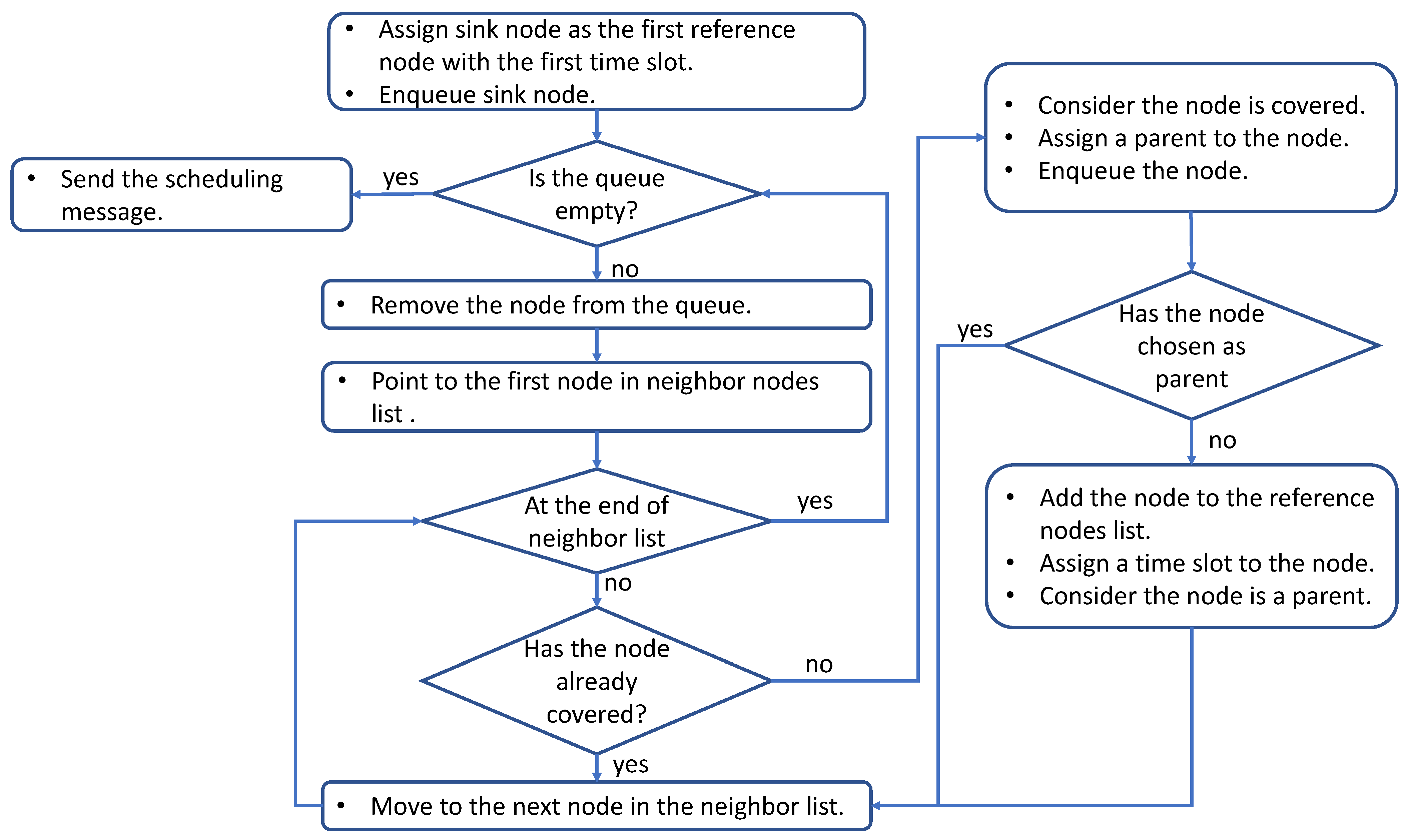
4. LPSRS Algorithm

LPSRS objects to decreasing power consumption while synchronizing the whole WSN. It actually uses a scheduling methodology that tries to cover as many nodes as possible with a small number of reference nodes. LPSRS consists of two processes: (1) the scheduling process and (2) the synchronization process. The scheduling process runs only during the configuration phase or when the network topologies are significantly altered. It offers a low-power approach to the aim of guaranteed synchronization for a tree-based network topology without collisions. Meanwhile, the synchronization step is repeated on a regular schedule with a $Psyn$ interval to keep the time offset of all nodes within an allowable threshold.

4.1. Scheduling Process

In this section, we explain in detail the scheduling algorithm, which aims to reduce communication costs while ensuring that all nodes in a tree-based network topology are completely covered. The suggested solution provides each reference node a distinct allocated time slot, ensuring that the synchronization operation is performed at a distinct time slot to avoid collisions.

We simply describe the core idea of the scheduling algorithm. Since finding the minimum list of connected reference nodes is an (NP)-hard problem [32], we simply use the breadth-first search (BFS) method to approximately find the minimum set of reference nodes. BFS is a method for traversing the graph layer. The total time complexity of BFS is $O\left(E+V\right)$ [33]. As the sink node (predefined node) has complete awareness of the system architecture, it simply uses BFS to identify the level of each node in the network. As shown in Figure 1 and Algorithm 1, the sink node begins from the sink node and finds out all the adjacent nodes at the current depth before moving on to the nodes at the next depth level (lines 8 to 12). The sink also determines all reference nodes, $RefNodes$, and their scheduled time slots, $SchSlots$ (lines 13 to 18). Here, $RefNodes$ are the nodes responsible to spread time messages to all nodes in the network. To prevent reusing the same reference node, we set $Paren{t}_{flag\left[j\right]}$ to a $true$ value (line 15). Next, all reference nodes and their related time slots are listed in the scheduling message. The scheduling message is then broadcast to all nodes in the network. To finish the synchronization process, each reference node uses its assigned time slot [21].

Algorithm 1: LPSRS pseudo-code for the scheduling process (sink node only).
$$\begin{gathered} \mathrm{Initial}:Q\leftarrow \varnothing ,CoverNode{s}_{flag[ ]}\leftarrow false,cnt\leftarrow 0, \\ Nod{e}_{Parent[ ]}\leftarrow \varnothing ,Paren{t}_{flag[ ]}\leftarrow false \end{gathered}$$
1.	$s\leftarrow sink node$
2.	$RefNodes\left(1\right)\leftarrow s$
3.	$Schslot\left(1\right)\leftarrow 0$
4.	$CoverNode{s}_{flag\left[s\right]}\leftarrow true$
5.	$enqueue\left(Q,s\right)$
6.	while$\left(Q!=Null\right)$do
7.	current i ← dequeue(Q); // Remove i form queue
8.	for (every edge (i, j) ∈ E) do
9.	if $\left(CoverNode{s}_{flag\left[j\right]}==false\right)$ Then
10.	$CoverNode{s}_{flag\left[j\right]}\leftarrow true$
11.	$Nod{e}_{Parent\left[j\right]}\leftarrow i$
12.	$enqueue\left(Q,j\right)$
13.	if $\left(Paren{t}_{flag\left[i\right]}==false\right)$ Then
14.	$RefNodes\left(cnt\right)\leftarrow i$
15.	$Paren{t}_{flag\left[j\right]}\leftarrow true$
16.	$SchSlots\left(cnt\right)\leftarrow cnt$
17.	cnt ← cnt + 1
18.	end if
19.	end if
20.	end for
21.	end while
22.	send scheduling message <0xFFFF, s, Sch, MesN, RefNodes, SchSlots, SeqN>

When a node receives a scheduling message, it applies Algorithm 2. Each node responds only if its ID has been stored in $RefNodes$ (lines 5 to 10). Then, it preserves the typically associated time slot, $mySchslot$. For each reference node, the waiting timer is initially started (WT) as soon as it receives the scheduling message. The value of WT can be computed as below:

$$WTvalue=mySchslot-Schslo{t}_{SrcID}$$

(1)

Here, $WTvalue$ is the amount of time each reference should wait before transmitting the scheduling message. $Schslo{t}_{SrcID}$ and $mySchslot$ are the sender’s time slot and the current reference time slot, respectively (lines 12 to 15). The current reference transmits the scheduling message to its nearby nodes as soon as WT eventually expires (lines 17 and 18). Additionally, each reference node examines the sequence number field, $SeqN$, to avoid sending the scheduling message multiple times. If the $SeqN$ of the current message is less than or equal to the $SeqN$ of the previous message, every reference node does not forward the message. It only adds the $SrcID$ of the sender node to its reference nodes neighbor list (lines 2 to 4). The reference nodes neighbor list is used by the synchronization process as described in Section 4.2.

Algorithm 2: LPSRS pseudo-code for the scheduling process (all nodes).
$Initial:cnt1\leftarrow 0,cnt2\leftarrow 0,sen{d}_{flag}\leftarrow false$, $SeqN\leftarrow 0$, $mySchsSlot\leftarrow 0$
1.	∎ Upon receiving Scheduling Message
2.	$\mathbf{if}\left(Received SeqN\le SeqN\right) \mathbf{Then}$
3.	$\mathrm{add} SenderID to RefNeighbors$ list
4.	end if
5.	$if \left(NodeID \mathrm{is} \mathrm{in} RefNodes\right) \mathbf{Then}$
6.	$cnt1\leftarrow \mathrm{position} \mathrm{of} NodeID \mathrm{in} RefNodes$
7.	$mySchsSlot\leftarrow SchSlots\left(cnt1\right)$
8.	$cnt2\leftarrow \mathrm{position} \mathrm{of} SenderID \mathrm{in} RefNodes$
9.	$SchSlo{t}_{SrcID}\leftarrow SchSlots\left(cnt2\right)$
10.	end if
11.	$WaitingTime\leftarrow \left(mySchSlot-SchSlo{t}_{SrcID}\right)$
12.	$\mathbf{if} (WaitingTime>0 \mathrm{and} sen{d}_{flag}==false) \mathbf{Then}$
13.	$sen{d}_{flag}\leftarrow true$
14.	Setup waiting timer $WT\left(WaitingTime\right)$
15.	end if
16.	$SeqN\leftarrow Received SeqN$
17.	∎ Upon WT expires
18.	send scheduling message <0xFFFF, NodeID, Sch, MesN, RefNodes, SchSlos, SeqN>

For a large network, if the size of $RefNodes$ and $SchSlots$ exceeds the maximum packet size, the scheduling message is divided into multiple small messages, $MesN$. Besides, the assigned time slot width of each reference node is increased to avoid collisions. It will be equal to $MesN$ times the time slot width. For example, if the maximum packet size is 50 bytes, the assigned time slot is 10 ms, and $RefNodes$ and $SchSlots$’s sizes are 80 bytes, the scheduling message is split into two messages, $MesN$ equals 2, and the time slot width is increased to be 20 ms.

In this paragraph, we clearly demonstrate an example of the suggested technique using the network represented in Figure 2. As illustrated in Figure 3, the sink node, $S,$ employs Algorithm 1 to construct a tree. It actually finds that the reference nodes are $S$ (sink node), $B$, $C$, $I$, and $F$ and that their allocated time slots are 0, 1, 2, 3, and 4, respectively (lines 6~21). Then, the sink node builds and broadcasts the scheduling message to its neighbor nodes (line 22). As a result, S fills the scheduling message as follows.

Upon receiving the scheduling message, each node uses Algorithm 2 to check the $SeqN$ (line 2). Here, the $SeqN$ = 1, which is greater than the previous $SeqN$ (default value = 0). As a result, each node examines whether or not it has been designated as a reference node. If it is a reference node, it sets its scheduled time slot to $mySchSlot$ and starts WT (lines 5~20). After the timeout expires, it sends the received packet. (Line 22). Node $C$, for example, is designated as a reference node, and the time slot is 2. $C$ then determines its waiting time, which is equal to 2. (2 ($C$’s $mySchSlot$)–0 ($Schslo{t}_{SrcID}$(sender node))). Next, $C$ delivers the received message to its adjacent nodes just as soon as the waiting timer expires.

4.2. Synchronization Process

In this section, we investigate and discuss the periodic synchronization process steps in detail. We conduct the synchronization process frequently, with a time period of $Psyn$ to conserve the time offset of all nodes within a suitable range (depending on the application). Once the scheduling process selects all reference nodes and their time slots, the synchronization process begins with the sink as the first reference node. The sink node’s time is considered the reference time to all surrounding nodes. The synchronization process consists of three simple steps that are repeated in each hierarchical level over a multi-hop network. Since each reference node has its own time slot, $Schslot$, it should perform the synchronization process within the scheduled time to avoid collisions. The synchronization process of LPSRS occurs in a single broadcast domain. R is the reference node, SIR is the specified reference node, and K represents the other neighbor’s nodes of R. Algorithm 3 and Figure 4 show how to estimate the total offset for frequent synchronization. In the first step, at time $T_{1,R}$, the $R=$ sink node broadcasts synchronization message number 1 ($Sync1$) to all its surrounding nodes. $Sync1$ includes the specified reference node, $SIR$, that has been randomly pre-selected (from the reference nodes neighbor list) by $SIR$ to send back a response (line 1 to 6).

Every node k $\in \mathbb{U}\left(R\right)$ saves the time stamp, $T_{2,k}$ for the arrival time of $Sync1$ (line 9). Here, $\mathbb{U}\left(R\right)$ denotes a group of nearby nodes inside the wireless range of $R$. Next, $SIR$ sends synchronization massage 2 ($Sync2$) back to $R$. $Sync2$ contains the arrival time of $Sync1$, $T_{2,SIR},$ as well as the time stamp for the transmit time, $T_{3,R},$ of $Sync2$ (line 10 to 13). Once $R$ gathers all time stamps $T_{1,R}$, $T_{2,SIR}$, $T_{3,SIR}$, and $T_{4,R}$ (the time right after receiving $Sync3$), $R$ estimates the offset by

$$O_{R,SIR}=\frac{\left(T_{2,SIR}+T_{3,SIR}\right)-\left(T_{4,R}+T_{1,R}\right)}{2}$$

(2)

Here, $O_{R,SIR}$ is the offset between $R$ and $SIR$. $R$ then broadcasts a synchronization message number ($Sync3$) to all its neighbor nodes, $k\in \mathbb{U}\left(R\right)$, which contains time $T_{2,SIR}$ and $O_{r,SIR}^{ }$ (line 18 to 23). Each node, $k,$ in $\mathbb{U}\left(R\right)$ receives $Sync3$ and checks the sequence number, $SeqN$. It only reacts if the current $SeqN$ in the message is higher than the previous one. Then, (line 26) it estimates the offset difference between $SIR$ and k, $O_{SIR,k}$, according to $SIR$ by

$$O_{SIR,k}=T_{2,SIR}-T_{2,k}$$

(3)

Then, (line 27) every node, $k,$ determines its total offset, $O_{R,k},$ as

$$O_{R,k}=O_{R,SIR}+O_{SIR,k}$$

(4)

Here, $O_{R,k}$ is the offset difference between $R$ and $k$. Finally, each node, $k,$ compensates its local time by subtracting the total offset, $O_{R,k},$ from its old local time, $T_k^{old}$, using

$$T_k^{new}=T_k^{old}-O_{R,k}$$

(5)

where $T_k^{old}$ denotes the old local time, and $T_k^{new}$ is the new local time of node $k$ (line 28). After all, the reference nodes within the wireless range of the sink node become synchronized and each reference node initiates the synchronization timer (ST) to repeat the same procedure until no further node can be synchronized (line 30 to 34). Each reference uses its time slot, $Schslot$, to avoid message collision.

For more clarification, we show an example of the synchronization method considering the depicted network in Figure 4. In the beginning, all nodes use Algorithm 3 for the synchronization process, and $S$ fills the synchronization message (Type: $Sync1$) as follows.

Next, it broadcasts $Sync1$ to all its neighbor nodes at the time $T_{1,\mathrm{S}}$. Since it has a list of neighbor reference nodes ($B$ and $C$), it selects node $B$ to be the responder (lines 1~7).

All nodes ($B, A, D, \mathrm{and} C$) receive $Sync1$ and keep the arrival time of $Sync1$ ($T_{2,B}, T_{2,A},T_{2,D}, \mathrm{and} T_{2,C}$) (line 9). Next, each reference node ($B \mathrm{and} C$) starts its own ST (lines 14~17). Node $B$ sends back $Sync2$ to node $S$. $Sync2$ consists of the arrival time of $Sync1$, $T_{2,B},$ as well as the time stamp for the transmit time, $T_{3,B}$, of $Sync2$ (lines 10~13). Node B sets the synchronization message as follows.

As soon as node $S$ receives the $Sync2$, it records the arrival time of $Sync2$, $T_{4,\mathrm{s}}$. Then, it calculates the offset using (2) and broadcasts $Sync3$ to all its neighbor nodes (lines 19–23). In addition, S fills the synchronization message (Type: $Sync3$) as follows.

Nodes ($B, A, D, \mathrm{and} C$) receive $Sync3$ and check $SeqN$. They find the $SeqN=1$ is higher than the previous one (default value = 0). Then, they estimate their offset and compensate their local time using (3), (4), and (5) (lines 25 to 29).

Nodes $B, C, I,$ and $F$ repeat the same process after their ST expires (lines 31 to 34). The synchronization process requires only three broadcast messages per reference node, regardless of the network size or density. Additionally, the scheduling process reduces the set of reference nodes. Thus, LPSRS can significantly reduce the number of message exchanges and is, therefore, well suited for low-power applications.

Algorithm 3: LPSRS pseudo-code for the synchronization process.
1.	$if \left(NodeID=sink node\right) Then$
2.	$R\leftarrow sink node$
3.	$SIR \leftarrow select rondlmly fromRefNeighbors list$
4.	$SeqN\leftarrow 1$
5.	$T_{1,R}$←$ReadCurrent Time$
6.	$send Sync1$ $<0\mathrm{xFFFF},R,SIR,Sync1,SeqN,-1,-1,-1,0>$
7.	end if
8.	∎ Upon receiving $Sync1$
9.	$T_{2,k}\leftarrow Read Current Time$ // $k$ represents all neighbor nodes of $R$
10.	$if \left(NodeID==SIR\right) Then$
11.	$T_{2,SIR}\leftarrow T_{2,k}$ $T_{3,SIR}\leftarrow Read Current Time$
12.	$send Sync2$ $<R,NodeID,-1,Sync2,SeqN,T_{2,SIR},T_{3,SIR},-1,0>$
13.	$end if$
14.	$if \left(NodeID \mathrm{is} \mathrm{in} RefNode\right) Then$
15.	$WaitingTime \leftarrow \left(mySchSlot-SchSlo{t}_{SrcID}\right)$
16.	Setup Synchronization timer $ST\left(WaitingTime\right)$
17.	$end if$
18.	∎ Upon receiving $Sync2$
19.	$if \left(NodeID==R\right) Then$
20.	$T_{4,R}\leftarrow Read Current Time$
21.	$O_{R,SIR}\leftarrow \left(\left(T_{2,SIR}+T_{3,SIR}\right)-\left(T_{4,R}-T_{1,R}\right)\right)/2$
22.	$send Sync3<0\mathrm{xFFFF},R,-1,Sync3,SeqN,-1,-1,T_{2,SIR},O_{R,SIR}>$
23.	$end if$
24.	∎ Upon receiving $Sync3$
25.	$if (Received SeqN>SeqN) Then$
26.	$O_{k,SIR}\leftarrow T_{2,SIR}-T_{2,k}$
27.	$O_{R,k}\leftarrow O_{R,SIR}+O_{NodeID,SIR}$
28.	$T_k^{new}\leftarrow T_k^{old}-O_{R,k}$
29.	$end if$
30.	∎ Upon ST expires
31.	$R\leftarrow NodeID$
32.	$SIR\leftarrow select rondlmly from RefNeighbors list$
33.	$T_{1,R}\leftarrow ReadCurrent Time$
34.	$send Sync1$ $<0\mathrm{xFFFF},R,SIR,Sync1,SeqN,-1,-1,-1,0>$

5. Experimental and Simulation Results

In this section, we present our achieved experimental results, followed by the simulation results. We have used the number of transmitted messages in each protocol during the synchronization process as the performance metric. Before discussing and explaining the experimental results, as described below, we show how the number of transmitted messages is the key performance indicator related to power consumption.

5.1. Power Consumption Analysis

In general, to analyze power consumption, we focus on the major power consumption caused by packet transmission and reception on sensor nodes. To save energy, wireless networks often cycle between sleep and active modes. As a result, power consumption is roughly proportional to the number of broadcasts and received packets, assuming a MAC-layer protocol that reduces idle listening time. Besides, wireless networks are broadcast domains [34]. As a result, for each broadcast, there are many receptions. Assume we have a wireless network with $N$ nodes that is equally distributed, with each node surrounded by $m$ nodes. The total power consumption, $P_T,$ can be expressed by transmission power, $P_{TX},$ and reception power, $P_{RX},$ as defined by

$$P_T=A\left(P_{TX}+m{P}_{RX}\right)\left(\frac{L}{D}\right)$$

(6)

where A indicates the number of transmitted messages, $L$ indicates the trace length in seconds, while $D$ indicates the duration of the message. The $P_{RX}$ has different modes. For example, NXP’s MCU with the RF transceiver chip KW01Z128 [35] has different modes. At the highest mode, the $P_{RX}$ is almost equal to $P_{TX}$. On the other hand, at the lowest mode, $P_{RX}$ is around 0.2 of $P_{TX}$. In this article, for sake of simplicity, we have chosen $P_{RX}\approx P_{TX}$. Since $P_{RX, }$ is almost equal to $P_{TX}$ [35], we can, therefore, simplify (6) into

$$P_T=A\frac{P_{TX}L\left(m+1\right)}{D}$$

(7)

According to (7), power usage is dependent on the number of messages sent, since the number of transmitted messages has a big impact on power consumption. In addition, we analyze the required number of the transmitted messages, $M$, for each protocol [35].

In R-sync, each node transmits a message to help build the spanning tree. The number of sent messages in the network is three times greater than the number of referenced links at the start of the time synchronization procedure. Additionally, there are further required messages for pulling isolated nodes. Thus, the total number of transmitted messages of R-Sync is: $M_{R\text{-}Sync}=N+3\left(R-1\right)+P$. Here $N$ is the node number, $R$ is the number of reference nodes, and $P$ is the number of pulling messages [9]. We note that $M_{R\text{-}Sync}$ is directly proportional to the number of nodes and the number of selected reference nodes.

Meanwhile, HRTS constructs a multi-level hierarchy of the network. At every level, each node sends two messages and obtains a response from the selected reference node. Therefore, the total number of transmitted messages of HRTS is $M_{HRTS}=2N+R$ [2]. $M_{HRTS}$ is directly proportional to the number of nodes [5].

Lastly, LPSRS requires $M_{LPSRS}=3\left(R-1\right)$ messages. However, LPSRS minimizes the number of reference nodes by using an efficient scheduling technique for the reference nodes. Besides, LPSRS is able to avoid collisions during its operations.

5.2. Experimental Results

The LPSRS protocol was built in C++ and implemented in an embedded CPU in the hardware sensors. We used the Arduino Nano RF (ANRF) as the hardware sensor. The ANRF utilizes an NRF24L01 RF transceiver and an ATmega328P CPU [36,37]. Moreover, it has a 2 kB memory and 32 KB Flash. The ANRF operated at a frequency of 2.4 GHz, and the bitrate was 50 kbps. We used 0 dBm as the transmitted power [38]. We created a testbed of 25 nodes, as shown in Figure 5, to build a wireless sensor network. For simplicity of the testing, with the help of the programming, we designed a wireless network of 3-way grid topology to test our protocol over a multi-hop network as depicted in Figure 6. In the 3-way grid topology, each node only receives incoming messages from nodes that have a common solid line. For example, in Figure 6, N12 only receives messages from N6, N7, N11, N13, N17, and N18. Therefore, we can evaluate LPSRS and other protocols under a realistic transmission contention and conditions of congestion.

Table 1. Comparison of LPSRS, R-sync, and HRTS.

LPSRS	R-sync	HRTS
42	57	64

shows the number of the transmitted message of LPSRS, R-sync, and HRTS for the network topology of Figure 6. It demonstrates that LPSRS, R-sync, and HRTS exchanged 42, 57, and 64 messages, respectively. LPSRS outperforms other technics (R-sync and HRTS). It can decrease the number of transmitted messages by around 26% and 35% compared to R-Sync and HRTS. Although the improvement in LPSRS looks moderate when compared to other protocols in the tiny test network shown in Figure 6, it develops fast as the network size increases. Due to the complexity of building large-scale actual hardware networks, we demonstrated this enhancement using simulations.

5.3. Simulation Results

To further test our proposed LPSRS protocol, we originally built a simulator that runs the LPSRS and HRTS algorithms. Meanwhile, the R-Sync simulation findings [9] have been adopted. In MATLAB, simulations were created employing wireless networks of varying sizes and ranges. We assumed the N sensor nodes were uniformly disrupted and scattered at random in a square area of 1000 m × 1000 m. Each node had a wireless communication range, denoted by $r$. We also presumed that all nodes were similar and self-contained. The sink node had two positions: (1) at the network’s center and (2) at the network’s corner. Due to the homogeneous distribution of the nodes, there was no significant change in the findings due to the position of the sink node. In this article, to prevent repetition, we only presented the findings if the sink node was placed in the network’s center, as other locations yielded similar results. In addition, we tested with LPSRS in the simulation using a wide variety of 12 distinct scenario networks, ranging from sparse to congested. We could simulate several different sorts of sensor nodes with varying wireless ranges by varying the transmission range. Changing the number of nodes in the network, on the other hand, allowed us to show the behavior of our protocol from a sparse network (200 nodes) up to a dense network (450 nodes).

Through simulations, we measured the number of transmitted messages in each protocol during the synchronization process, which is the key performance indicator related to power consumption. As described in Section II, HRTS and R-Sync often incur a large number of collisions during the synchronization process, while LPSRS is guaranteed to have no collisions. For the sake of simplicity, we assumed that no collisions happen even in HRTS and R-Sync.

Figure 7 depicts the number of messages delivered by all three protocols (LPSRS, R-Sync, and HRTS) across a range of network different sizes from 200 to 450 nodes. For a large network with 450 nodes, it can be seen that R-Sync and HRTS generated 970 messages and 1071 messages, respectively. On the other hand, LPSRS generated around 500 messages. That is, LPSRS outperformed the other two protocols, as it decreased the number of transmitted messages to around 49% and 53% compared to R-Sync and HRTS, respectively.

Figure 8 shows the number of transmitted messages under different communication ranges from 85 m to 160 m. It can be found that LPSRS substantially outperformed the other methods. For a network with a communication range of 85m, LPSRS decreased the number of transmitted messages to around 55% and 34% compared to R-Sync and HRTS, respectively. On the other hand, for a network with a long communication range of 160 m, LPSRS generates around 175 messages. LPSRS outperformed HRTS and R-Sync by a factor of around 3 and 1.4, respectively.

Based on the results presented above, it is reasonable to conclude that LPSRS consumes less energy than the other techniques. LPSRS, on the other hand, does not compromise timing accuracy. The offset calculations described by HRTS [12] and DTSync [7] during the synchronization process were used, which is recognized to provide high timing accuracy. For more details, we compared DTSync and HRTS in our previous work with more protocols (see Table 11 [11]). Furthermore, LPSRS can manage high-density networks without losing its key features, making it a highly scalable and flexible protocol.

6. Conclusions

In this article, we suggested LPSRS as a time synchronization protocol for the IoT. It addressed the power consumption and collision issues in IoT networks. LPSRS significantly decreased the number of messages, resulting in significant power savings. We constructed LPSRS into a real wireless sensor network with different configurations and an extensive simulation with large-scale networks. According to the experimental results, LPSRS requires fewer messages than prior approaches such as R-Sync and HRTS. It can decrease the number of transmitted messages by around 26% and 35% compared to R-Sync, and this benefit, in turn, reduces LPSRS’s energy use. In addition, we can consider LPSRS as a semi-centralized synchronization protocol, as some tasks are completed by the sink node and other tasks are completed locally by each node. Therefore, LPSRS is very convenient for those applications in which the network topology is recognized, e.g., smart metering.

References

- Farzad, A.; Najafi, K. BlueSync: Time Synchronization in Bluetooth Low Energy with Energy Efficient Calculations. IEEE Internet Things J. 2021. [Google Scholar] [CrossRef]
- Xintao, H.; Kim, K.S.; Lee, S.; Lim, E.G.; Marshall, A. Improving Multi-Hop Time Synchronization Performance in Wireless Sensor Networks Based on Packet-Relaying Gateways with Per-Hop Delay Compensation. IEEE Trans. Commun. 2021, 69, 6093–6105. [Google Scholar]
- Phan, L.-A.; Kim, T.; Kim, T. Robust neighbor-aware time synchronization protocol for wireless sensor network in dynamic and hostile environments. IEEE Internet Things J. 2020, 8, 1934–1945. [Google Scholar] [CrossRef]
- ElSharief, M.; El-Gawad, M.A.A.; Ko, H.; Pack, S. EERS: Energy-Efficient Reference Node Selection Algorithm for Synchronization in Industrial Wireless Sensor Networks. Sensors 2020, 20, 4095. [Google Scholar] [CrossRef] [PubMed]
- Sarvghadi, M.A.; Wan, T.-C. Message passing based time synchronization in wireless sensor networks: A survey. Int. J. Distrib. Sens. Netw. 2016, 12, 1280904. [Google Scholar] [CrossRef]
- Yildirim, K.S.; Kantarci, A. Time synchronization based on slow-flooding in wireless sensor networks. IEEE Trans. Parallel Distrib. Syst. 2013, 25, 244–253. [Google Scholar] [CrossRef]
- ElSharief, M.; El-Gawad, M.A.A.; Kim, H.W. Density table-based synchronization for multi-hop wireless sensor networks. IEEE Access 2017, 6, 1940–1953. [Google Scholar] [CrossRef]
- Choudhury, N.; Matam, R.; Mukherjee, M.; Shu, L. Beacon synchronization and duty-cycling in IEEE 802.15. 4 cluster-tree networks: A review. IEEE Internet Things J. 2018, 5, 1765–1788. [Google Scholar] [CrossRef]
- Qiu, T.; Zhang, Y.; Qiao, D.; Zhang, X.; Wymore, M.L.; Sangaiah, A.K. A robust time synchronization scheme for industrial internet of things. IEEE Trans. Ind. Inform. 2018, 14, 3570–3580. [Google Scholar] [CrossRef]
- Yildirim, K.S. Gradient descent algorithm inspired adaptive time synchronization in wireless sensor networks. IEEE Sens. J. 2016, 16, 5463–5470. [Google Scholar] [CrossRef]
- EMahmoud, l.; El-Gawad, M.A.A.; Kim, H. Fads: Fast scheduling and accurate drift compensation for time synchronization of wireless sensor networks. IEEE Access 2018, 6, 65507–65520. [Google Scholar]
- Hui, D.; Han, R. TSync: A lightweight bidirectional time synchronization service for wireless sensor networks. ACM SIGMOBILE Mob. Comput. Commun. Rev. 2004, 8, 125–139. [Google Scholar]
- Miklós, M.; Kusy, B.; Simon, G.; Lédeczi, Á. The flooding time synchronization protocol. In Proceedings of the 2nd International Conference on Embedded Networked Sensor Systems, Baltimore, MD, USA, 3–5 November 2004; pp. 39–49. [Google Scholar]
- Lenzen, C.; Sommer, P.; Wattenhofer, R. PulseSync: An efficient and scalable clock synchronization protocol. IEEE/ACM Trans. Netw. 2015, 23, 717–727. [Google Scholar] [CrossRef]
- Lenzen, C.; Sommer, P.; Wattenhofer, R. Optimal clock synchronization in networks. In Proceedings of the 7th ACM Conference on Embedded Networked Sensor Systems, Berkeley, CA, USA, 4–6 November 2009; pp. 225–238. [Google Scholar]
- Yildirim, K.S.; Gurcan, O.; Yildirim, K.S. Efficient time synchronization in a wireless sensor network by adaptive value tracking. IEEE Trans. Wirel. Commun. 2014, 13, 3650–3664. [Google Scholar] [CrossRef][Green Version]
- Elson, J.; Girod, L.; Estrin, D. Fine-grained network time synchronization using reference broadcasts. ACM SIGOPS Oper. Syst. Rev. 2002, 36, 147–163. [Google Scholar] [CrossRef]
- Gong, F.; Sichitiu, M.L. CESP: A low-power high-accuracy time synchronization protocol. IEEE Trans. Veh. Technol. 2016, 65, 2387–2396. [Google Scholar] [CrossRef]
- Saurabh, G.; Kumar, R.; Srivastava, M.B. Timing-sync protocol for sensor networks. In Proceedings of the 1st International Conference on Embedded Networked Sensor Systems, New York, NY, USA, 5–7 November 2003; pp. 138–149. [Google Scholar]
- Leandro, T.B.; Heimfarth, T.; de Freitas, E.P. Enhancing time synchronization support in wireless sensor networks. Sensors 2017, 17, 2956. [Google Scholar]
- ElSharief, M.A.; El-Gawad, M.A.A.; Kim, H.; El-Gawad, M.A. Low-Power Scheduling for Time Synchronization Protocols in a Wireless Sensor Networks. IEEE Sens. Lett. 2019, 3, 1–4. [Google Scholar] [CrossRef]
- Atis, E.; Fafoutis, X.; Duquennoy, S.; Oikonomou, G.; Piechocki, R.; Craddock, I. Temperature-resilient time synchronization for the internet of things. IEEE Trans. Ind. Inform. 2017, 14, 2241–2250. [Google Scholar]
- Luca, S.; Gamba, G. A distributed consensus protocol for clock synchronization in wireless sensor network. In Proceedings of the 2007 46th IEEE Conference on Decision and Control, New Orleans, LA, USA, 12–14 December 2007. [Google Scholar]
- Panigrahi, N.; Khilar, P. Multi-hop consensus time synchronization algorithm for sparse wireless sensor network: A distributed constraint-based dynamic programming approach. Ad Hoc Netw. 2017, 61, 124–138. [Google Scholar] [CrossRef]
- Jianshe, W.; Jiao, L.; Ding, R. Average time synchronization in wireless sensor networks by pairwise messages. Comput. Commun. 2012, 35, 221–233. [Google Scholar]
- Maggs, M.K.; O’Keefe, S.G.; Thiel, D. Consensus clock synchronization for wireless sensor networks. IEEE Sens. J. 2012, 12, 2269–2277. [Google Scholar] [CrossRef]
- Phan, L.-A.; Kim, T. Fast consensus-based time synchronization protocol using virtual topology for wireless sensor networks. IEEE Internet Things J. 2021, 8, 7485–7496. [Google Scholar] [CrossRef]
- Shi, F.; Tuo, X.; Ran, L.; Ren, Z.; Yang, S.X. Fast convergence time synchronization in wireless sensor networks based on average consensus. IEEE Trans. Ind. Inform. 2020, 16, 1120–1129. [Google Scholar] [CrossRef]
- Lim, H.; Kumar, S.; Kim, H. Density-driven scheduling of low power synchronization for wireless sensor networks. In Proceedings of the 2016 International Conference on Electronics, Information, and Communications (ICEIC), Danang, Vietnam, 27–30 January 2016. [Google Scholar]
- Ranjan, R.; Varma, S. Collision-free time synchronization for multi-hop wireless sensor networks. J. Comput. Intell. Electron. Syst. 2012, 1, 200–206. [Google Scholar] [CrossRef]
- Ranjan, R.; Varma, S. Challenges and implementation on cross layer design for wireless sensor networks. Wirel. Pers. Commun. 2016, 86, 1037–1060. [Google Scholar] [CrossRef]
- Kim, D.; Wu, Y.; Li, Y.; Zou, F.; Du, D.-Z. Constructing Minimum Connected Dominating Sets with Bounded Diameters in Wireless Networks. IEEE Trans. Parallel Distrib. Syst. 2008, 20, 147–157. [Google Scholar]
- Cormin, T.; Leiserson, C.E.; Rivest, R.L.; Stein, C. Introduction to Algorithms; MIT Press: Cambridge, MA, USA, 2009. [Google Scholar]
- IEEE Std 802.15.4-2015; IEEE Standard for Low-Rate Wireless Networks. IEEE Standards Association: Piscataway, NJ, USA, 2016; Volume 802.
- NXP. MKW01Z128 Highly-Integrated, Cost-Effective Single-Package Solution for Sub-1 GHz applications. Document Number: MKW01Z128, Rev. 5,03/2014. Available online: http://www.nxp.com (accessed on 5 December 2021).
- Arduino Nano User Manual. Available online: https://www.arduino.cc/en/uploads/Main/ArduinoNanoManual23.pdf (accessed on 5 January 2022).
- nRF24L01+ Preliminary Product Specification. Available online: https://www.sparkfun.com/datasheets/Components/SMD/nRF24L01Pluss_Preliminary_Product_Specification_v1_0.pdf (accessed on 5 January 2022).
- ATmega328P [DATASHEET]. Available online: http://ww1.microchip.com/downloads/en/DeviceDoc/Atmel-7810-Automotive-Microcontrollers-ATmega328P_Datasheet.pdf (accessed on 5 January 2022).