Robust Scheduling of Networked Microgrids for Economics and Resilience Improvement

Abstract

The benefits of networked microgrids in terms of economics and resilience are investigated and validated in this work. Considering the stochastic unintentional islanding conditions and conventional forecast errors of both renewable generation and loads, a two-stage adaptive robust optimization is proposed to minimize the total operating cost of networked microgrids in the worst scenario of the modeled uncertainties. By coordinating the dispatch of distributed energy resources (DERs) and responsive demand among networked microgrids, the total operating cost is minimized, which includes the start-up and shut-down cost of distributed generators (DGs), the operation and maintenance (O&M) cost of DGs, the cost of buying/selling power from/to the utility grid, the degradation cost of energy storage systems (ESSs), and the cost associated with load shedding. The proposed optimization is solved with the column and constraint generation (C&CG) algorithm. The results of case studies demonstrate the advantages of networked microgrids over independent microgrids in terms of reducing total operating cost and improving the resilience of power supply.

1. Introduction

A microgrid could be seen as a controllable local energy system consisting of various distributed generators (DGs), energy storage systems (ESSs), and energy consumers. Normally, a microgrid is connected to a utility grid through the Point of Common Coupling (PCC) but has the capability of operating independently [1]. When connected to the utility grid, a microgrid can not only import power from or export power to the utility distribution network under different operational conditions, but also provide various kinds of ancillary services, e.g., frequency regulation, voltage support, virtual inertia, etc., to the utility grid [2,3,4]. For energy consumers, a microgrid can reduce carbon emission, improve energy efficiency, and serve low-cost and clean energy. In particular, through intentionally/unintentionally islanding from the utility grid, a microgrid is able to continue to supply power to its customers without any interruption when there is an outage on the utility gird, leading to improved energy resilience [5]. Because of these advantages, the study on microgrids has never been more popular [6].

While the benefits of individual microgrids for improving the resilience of local power supply and facilitating integration of renewable generation have been well recognized, networked microgrids, defined as the aggregation of adjacent microgrids that are physically connected and functionally interoperable, provide a more efficient and resilient alternative. Generally, a microgrid imports/exports power from/to the distribution grid in grid-connected mode, and this power is instantaneously forced to be zero when unintentional islanding happens. In this circumstance, the islanding process needs quick adjustment of the already committed DGs and ESSs, and even load shedding as the last resort to mitigate the power imbalance caused by unintentional islanding. To reduce or avoid load shedding and have the microgrid being prepared for possible unintentional islanding, certain number of DGs should be installed and committed and the ESSs should be oversized and charged to certain levels. Under this circumstance, interconnecting separate microgrids into networked microgrids has the potential to reduce the installed capacity of DGs and ESSs by sharing DGs and ESSs as well as loads with diverse profiles. In addition, networked microgrids can improve the resilience of power supply through exchanging power during grid outages or reducing the total operating cost under the same level of resilience. Due to such benefits, networked microgrids have attracted growing attention [7].

1.1. Literature Review and Gap Analysis

Existing research works are mostly focused on the multi-level energy management of networked microgrids for economic benefits and networked-microgrid-assisted restoration and recovery for resilience. In [8], a bi-level scheduling strategy for coordinated operation of networked microgrids in a distribution system is proposed. Each microgrid performs its own energy management in the lower level, while a robust economic dispatch model for distribution system is formulated in the upper level, through which price signals are derived and then sent to each microgrid. In [9], a nested energy management strategy is proposed for day-ahead scheduling of networked microgrids. In [10], a distributed energy management framework is proposed for a collaborative operation of networked microgrids and the local utility grid. Compared with centralized energy management in [8,9], distributed energy management guarantees cooperation among microgrids with fairness and privacy while addressing the issue of scalability of energy management in networked microgrids. In [11], a decentralized energy management system is proposed for networked hybrid AC/DC microgrids. The energy sharing of networked microgrids is coordinated by the DC network to minimize the power transmission loss with network constraints. These research studies are mainly focused on optimizing the energy transactions between microgrids for economic benefit. However, the stochasticity of unintentional islanding has been ignored, i.e., the resiliency benefit of networked microgrids is rarely considered in the existing energy management models.

Since microgrids are usually connected at the distribution level, the resiliency benefits of networked microgrids are mostly demonstrated through facilitating the restoration and recovery of the distribution system [12,13]. Based on the roles that networked microgrids could play, networked microgrids assist in the restoration and recovery of distribution grids mainly from three aspects: networked-microgrid-assisted restoration [14,15], networked-microgrid-assisted network formation [16,17], and networked-microgrid-assisted blackstart [18,19]. However, the implementation of these networked-microgrid-assisted strategies requires significant changes to today’s existing regulatory environments [20]. Further, effectiveness of these strategies requires oversized DGs and ESSs in microgrids. In other words, the resiliency benefits are gained at the expense of sacrificing the economic benefits.

In fact, the economic benefits of networked microgrids cannot be verified without considering the resilience, and vice versa. For this reason, it is necessary to consider the stochasticity of unintentional islanding in the energy management of networked microgrids since the most fundamental feature of microgrids is to seamlessly separate from the distribution system during outages and continue to supply its islanded portion. In [21], the islanding capability of a microgrid is modeled as a chance constraint and integrated into the stochastic microgrid scheduling problem. The chance-constrained programming model is extended to include the reconfiguration of microgrids in [22]. In [23], the probability distribution of islanding duration is estimated and modeled by a scenario set. Nevertheless, the generation of scenario sets needs a probability distribution of unscheduled islanding periods, on which information is very limited in practice. Unlike stochastic optimization, robust optimization only needs the upper and lower boundaries of the stochastic variables, neglecting their probability distributions and correlations. In [24], a robust optimization model is proposed to quantify the reserve requirements of microgrids. Considering resiliency requirements, another robust optimization model is proposed for microgrid scheduling in [25]. However, the occurrence time of the unintentional islanding has to be enumerated. Further, the power balance is only required for a very short adjusting time (e.g., 5 min) after islanding, and the duration of the unintentional islanding have been neglected. In [26], the pre-set multi-period islanding constraints are included in the microgrid scheduling model. In [27], the uncertainties of renewable generation and grid-connection condition are included in the microgrid scheduling problem by formulating a two-stage robust optimization model. However, the uncertainty of load and the choice of load shedding have been ignored. Nevertheless, refs. [21,22,23,24,25,26,27] are all targeted at a single microgrid.

To summarize, the advantages of networked microgrids over independent microgrids cannot be verified without considering both the economic and resiliency aspects. Research studies in [8,9,10,11] optimize the energy transactions between microgrids for economic benefits while ignoring the stochasticity of unintentional islanding; i.e., the resiliency benefits of networked microgrids are not considered. In [12,13,14,15,16,17,18,19,20], the resiliency benefits of networked microgrids are demonstrated through facilitating the restoration and recovery of distribution grids, which leads to unnecessarily oversized DGs and ESSs. Considering the most fundamental feature of microgrids is seamlessly islanding from the distribution system during outages and continuing to supply its islanded portion, the islanding capability of a microgrid is proposed to be integrated into the stochastic microgrid scheduling in [21,22,23] and robust microgrid scheduling in [24,25,26,27]. However, the occurrence time and duration of the unintentional islanding have been either pre-set or neglected. In addition, studies in [21,22,23,24,25,26,27] are all focusing on a single microgrid.

To verify the advantages of networked microgrids over independent microgrids in terms of both economics and resilience, a two-stage adaptive robust optimization is proposed to minimize the total operating cost of networked microgrids considering the stochastic occurrence time and duration of the unintentional islanding conditions and conventional forecast errors of both renewable generation and loads. By coordinating the dispatch of distributed energy resources (DERs) and responsive demand among networked microgrids, the advantages of networked microgrids over independent microgrids are validated in terms of both reducing the operating cost and improving the resilience of power supply.

1.2. Contributions and Outline

In this paper, given the stochastic unintentional islanding conditions, a robust optimization model is proposed for optimal scheduling of networked microgrids. The proposed model is guaranteed to serve local loads continuously through rapidly adjusting the output of committed DGs and ESSs and leveraging various DGs and ESSs from networked microgrids whenever unintentional islanding happens. To capture the uncertainties in renewable generation, demand, and the occurrence time and duration of the unintentional islanding, a two-stage adaptive robust optimization is proposed to optimize the objective function in the worst-case scenario of the modeled uncertainties. The proposed optimization is solved with the column and constraint generation (C&CG) algorithm. The results obtained demonstrate the advantages of networked microgrids over independent microgrids in terms of reducing the operating cost and improving the resilience of power supply. The main contributions of this work are threefold:

1.

Considering the uncertainties of the occurrence time and duration of the unintentional islanding, a two-stage robust optimization for optimal scheduling of networked microgrids is proposed to guarantee local loads being served continuously through rapidly adjusting the output of committed DGs and ESSs in case of unintentional islanding.

2.

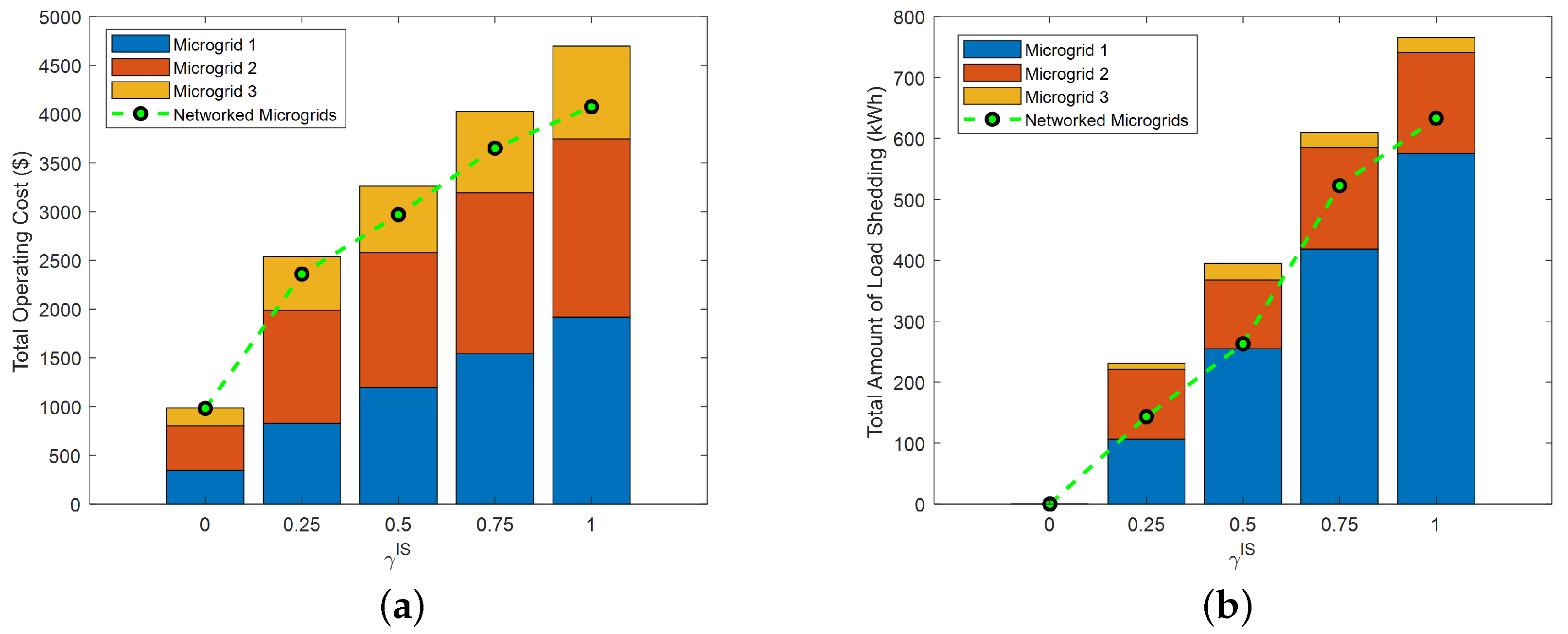
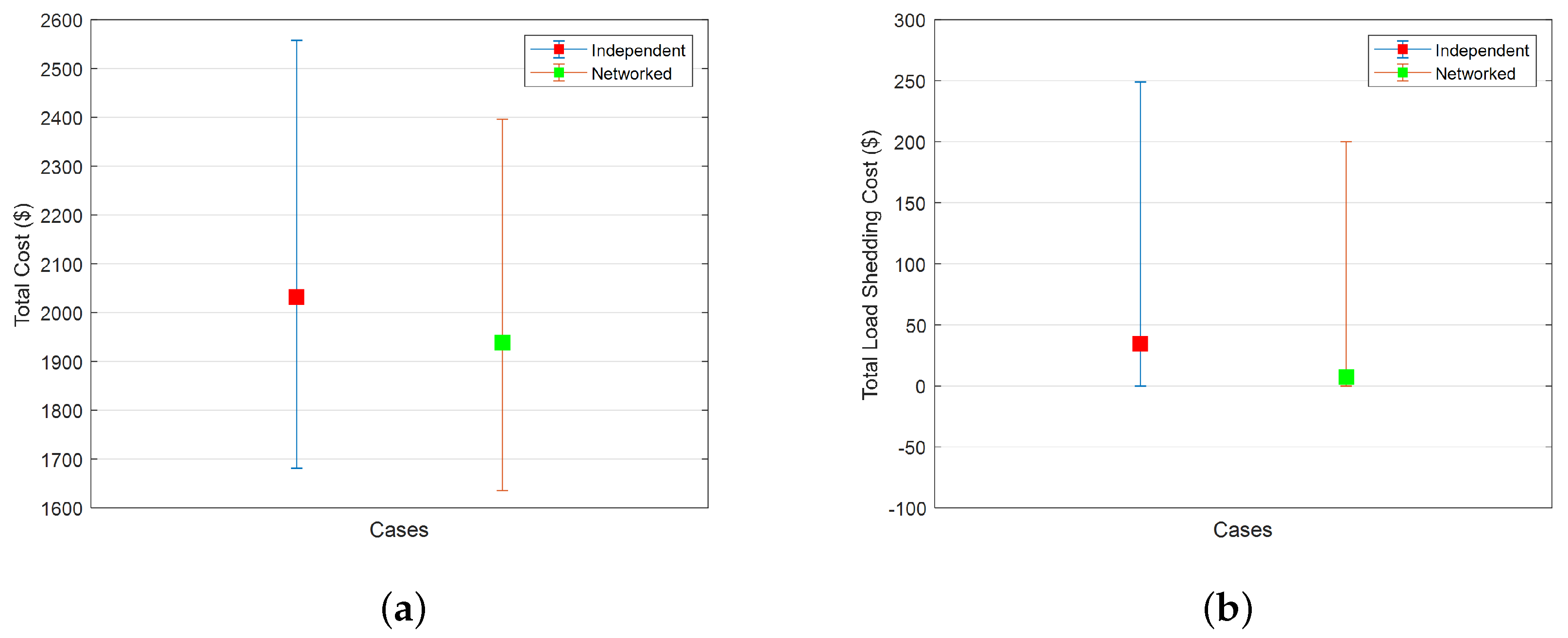
The correctness and effectiveness of proposed robust optimization model are validated through various case studies. In particular, the advantages of networked microgrids over independent microgrids in terms of reducing the operating cost and improving the resilience of power supply have been verified.

3.

The solution efficiency of the C&CG algorithm in large and networked microgrids has been validated.

This paper is structured as follows: The modeling of microgrid components and networked microgrids is presented in Section 2. Section 3 describes the proposed two-stage robust optimization model for networked microgrid scheduling considering the stochastic unintentional islanding conditions. The numerical simulation results and analysis are given in Section 4. The paper is concluded with major findings in Section 5.

2. Modeling

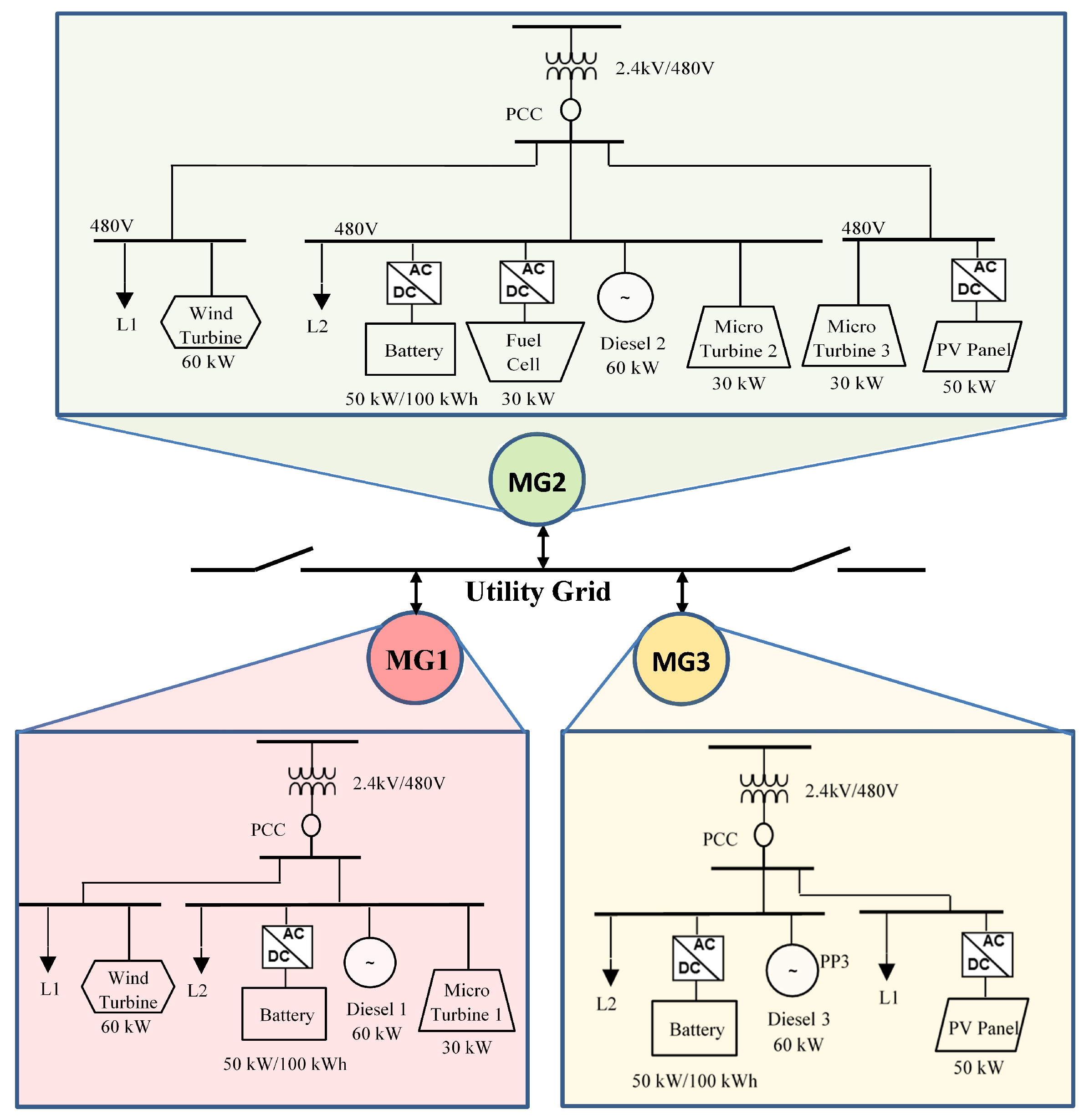
2.1. Microgrid Components

A microgrid consists of various distributed generators (DGs), ESSs, and energy consumers. In practice, a microgrid central control (MCC) monitors the system running status and sends optimize dispatch orders to corresponding components. The DGs in a microgrid simply fall into two categories: dispatchable and undispatchable. Dispatchable DGs, e.g., small hydros, fuel cells, and microturbines, could be dispatched on demand at the request of MCC based on market needs or operator’s preference. By contrast, undispatchable DGs, mainly referring to wind power and PV, are subject to the uncertain nature of weather conditions and thus cannot be completely controlled by the MCC. In fact, wind power and PV power can only be forecasted with limited accuracy. For wind power, the hour-ahead forecast error could be made below 10%. However, the day-ahead forecast error is generally over 20% [28,29]. As to PV power forecasting, the problem is getting more difficult due to random cloud coverage and changing ambient temperature, both of which affect the PV generation significantly [30,31]. To mitigate the uncertainties of renewables, ESSs are normally installed on-site. Without loss of generality, both wind and PV power are assumed independent and bounded random variables in this work. The goal here is to guarantee continuous power supply of local demands through seamless islanding considering the uncertainties of renewables, load, and the occurrence time and duration of the unintentional islanding.

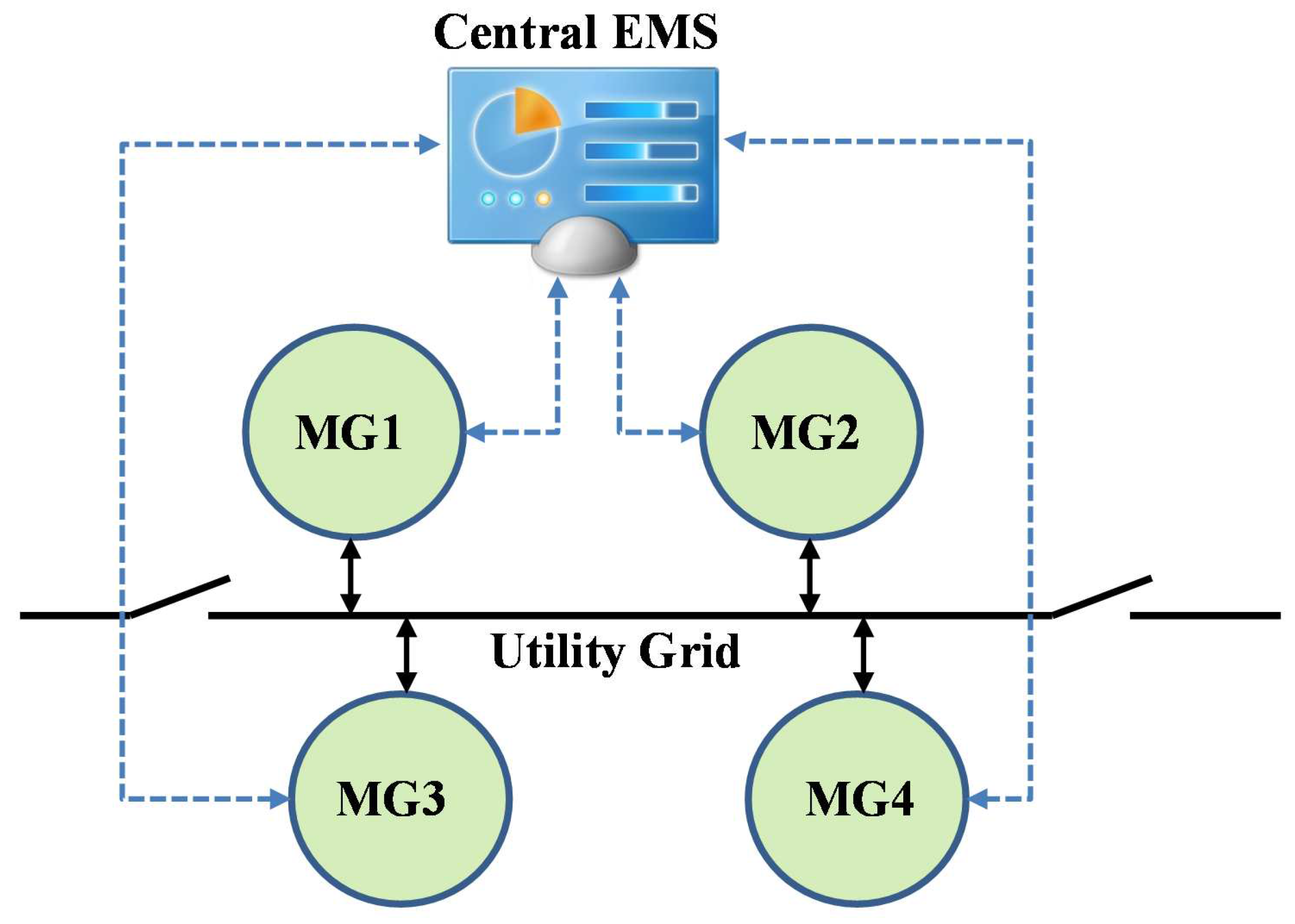
2.2. Networked Microgrids Structure

Traditionally, microgrids are rare and scattered thinly in the distribution grid. Each microgrid is an independent and autonomous entity that has the choice to disconnect from the distribution grid and perform as an autonomous island when the distribution grid is disturbed. As more microgrids have been deployed in recent years, multiple microgrids are becoming geographically adjacent and physically connected. Nevertheless, these connected microgrids might still be functionally independent, i.e., independent microgrids. Alternatively, these interconnected adjacent microgrids could also be networked at the communication and control layers and become functionally interoperable networked microgrids. A simple illustration of networked microgrids is shown in Figure 1, which consists of four individual microgrids. A central energy management system (EMS) communicates with individual microgrids and coordinates the dispatch of them. Whenever the upstream or downstream feeder is outaged, the two switches are opened and the four microgrids become an island of networked microgrids. By sharing DGs and ESSs as well as loads with diverse profiles, networked microgrids are expected to achieve better economics and resilience compared with independent microgrids.

3. Mathematical Formulation

3.1. Robust Optimization Model

In this section, the networked microgrids scheduling problem is modeled as a two-stage robust optimization by considering the variation of renewable generation, load, and grid-connection condition. Unlike stochastic optimization, robust optimization does not require the probability distributions and correlations of the stochastic variables. Without loss of generality, wind power $P_{mwt}^{\mathrm{W}}$, PV power $P_{mvt}^{\mathrm{PV}}$, and load $P_{mdt}^{\mathrm{L}}$ are all assumed independent, symmetric, and continuous random variables as in (1). Meanwhile, the grid-connection condition $Z_t^{\mathrm{G}}$ is assumed to be a binary random variable. Since these microgrids are geographically adjacent and physically connected to the same substation or feeder, the grid-connection condition $Z_t^{\mathrm{G}}$ is assumed same for all microgrids. Meanwhile, the wind and PV power between microgrids are assumed perfect positive correlated.

$$\left\{\begin{array}{cc}{P}_{mwt}^{\mathrm{W}}\in \left[P_{mwt}^{\hat{\mathrm{W}}}-{\delta }_{mwt}^{\mathrm{W}},P_{mwt}^{\hat{\mathrm{W}}}+{\delta }_{mwt}^{\mathrm{W}}\right]\hfill & {\delta }_{mwt}^{\mathrm{W}}\ge 0\hfill \\ P_{mvt}^{\mathrm{PV}}\in \left[P_{mvt}^{\hat{\mathrm{P}}\mathrm{V}}-{\delta }_{mvt}^{\mathrm{PV}},P_{mvt}^{\hat{\mathrm{P}}\mathrm{V}}+{\delta }_{mvt}^{\mathrm{PV}}\right]\hfill & {\delta }_{mvt}^{\mathrm{PV}}\ge 0\hfill \\ P_{mdt}^{\mathrm{L}}\in \left[P_{mdt}^{\hat{\mathrm{L}}}-{\delta }_{mdt}^{\mathrm{L}},P_{mdt}^{\hat{\mathrm{L}}}+{\delta }_{mdt}^{\mathrm{L}}\right]\hfill & {\delta }_{mdt}^L\ge 0\hfill \\ Z_t^{\mathrm{G}}\in \left\{0,1\right\},\hfill & \forall m,w,v,d,t\hfill \end{array}\right.$$

(1)

The model is targeted to minimize total operating cost of the networked microgrids as shown in (2), including start-up, shut-down, and fixed operation and maintenance (O&M) cost of DGs (as in the first line), variable O&M cost of DGs (as in the third line), cost of buying/selling power from/to utility grid (as in the fourth line), degradation cost of ESSs (as in the fifth line), and cost associated with load shedding (as in the sixth line). The robust optimization model is formulated in “min-max-min” form, as presented in (2)–(12). The commitment status of DGs is determined in the first stage before the realization of uncertainties and keeps the same value for all possible realizations of uncertainties. The second-stage decisions, i.e., the PCC power, DG and ESS power, and load shedding, are changing based on the worst realization of renewable generation, load, and grid-connection conditions. By searching and optimizing the worst scenario, the proposed robust optimization guarantees the feasibility and bottom line of the solution under all possible realizations of uncertainties.

$$\begin{array}{ccc}\hfill \underset{\mathbf{u}\in \mathbb{U}}{\min }& & \sum _{t=1}^{N_T}\sum _{m=1}^{N_M}\sum _{i=1}^{N_{mG}}{S}_{mit}^{\mathrm{U}}+S_{mit}^{\mathrm{D}}+C_{mit}^{\mathrm{ON}}{u}_{mit}\hfill \\ & & +\underset{{\mathbf{Z}}^{\mathbf{G}},{\mathbf{P}}^{\mathrm{W}},{\mathbf{P}}^{\mathrm{PV}},{\mathbf{P}}^{\mathrm{L}}\in \mathbb{W}}{\max }\underset{\mathbf{P},{\mathbf{P}}^{\mathbf{PCC}},{\mathbf{P}}^{\mathbf{C}},{\mathbf{P}}^{\mathbf{D}},{\mathbf{P}}^{\mathbf{LS}}\in \mathbb{X}}{\min }\hfill \\ & & \left\{\sum _{t=1}^{N_T}\sum _{m=1}^{N_M}\sum _{i=1}^{N_{mG}}{\lambda }_{mit}{P}_{mit}\right.\hfill \\ & & +\sum _{t=1}^{N_T}\sum _{m=1}^{N_M}{\lambda }_{mt}^{\mathrm{PCC}}{P}_{mt}^{\mathrm{PCC}}\hfill \\ & & +\sum _{t=1}^{N_T}\sum _{m=1}^{N_M}\sum _{b=1}^{N_{mB}}{C}_{mbt}\left(P_{mbt}^{\mathrm{C}}+P_{mbt}^{\mathrm{D}}\right)\hfill \\ & & \left.\sum _{t=1}^{N_T}\sum _{m=1}^{N_M}\sum _{d=1}^{N_{mD}}{C}_{mdt}^{\mathrm{LS}}{P}_{mdt}^{\mathrm{LS}}\right\}\hfill \end{array}$$

(2)

s.t.

$$\mathbb{U}=\left\{\mathbf{u}:u_{mit}\in \left\{0,1\right\},\forall m,\forall i,t;\right\}$$

(3)

$$\begin{array}{ccc}\hfill \mathbb{W}& =& \left\{{\mathbf{P}}^{\mathrm{W}}:P_{mwt}^{\mathrm{W}}=P_{mwt}^{\hat{\mathrm{W}}}-\underline{{\mu }_{mwt}}{\delta }_{mwt}^{\mathrm{W}}+\overline{{\mu }_{mwt}}{\delta }_{mwt}^{\mathrm{W}},\forall m,\forall w,t\right.\hfill \\ & & {\mathbf{P}}^{\mathrm{PV}}:P_{mvt}^{\mathrm{PV}}=P_{mvt}^{\hat{\mathrm{P}}\mathrm{V}}-\underline{{\mu }_{mvt}}{\delta }_{mvt}^{\mathrm{PV}}+\overline{{\mu }_{mvt}}{\delta }_{mvt}^{\mathrm{PV}},\forall m,\forall v,t\hfill \\ & & {\mathbf{P}}^{\mathrm{L}}:P_{mdt}^{\mathrm{L}}=P_{mdt}^{\hat{\mathrm{L}}}-\underline{{\mu }_{mdt}}{\delta }_{mdt}^{\mathrm{L}}+\overline{{\mu }_{mdt}}{\delta }_{mdt}^{\mathrm{L}},\forall m,\forall d,t\hfill \\ & & \underline{{\mu }_{mwt}},\overline{{\mu }_{mwt}},\underline{{\mu }_{mvt}},\overline{{\mu }_{mvt}},\underline{{\mu }_{mdt}},\overline{{\mu }_{mdt}}\in \left[0,1\right],\forall m,\forall w,v,d,t\hfill \\ & & \sum _{w=1}^{N_{mW}}\left(\underline{{\mu }_{mwt}}+\overline{{\mu }_{mwt}}\right)+\sum _{v=1}^{N_{mPV}}\left(\underline{{\mu }_{mvt}}+\overline{{\mu }_{mvt}}\right)\hfill \\ & & +\sum _{d=1}^{N_{mD}}\left(\underline{{\mu }_{mdt}}+\overline{{\mu }_{mdt}}\right)\le {\Gamma }_{mt}^{\mathrm{P}},\forall m\forall t\hfill \\ & & {\mathbf{Z}}^{\mathbf{G}}:\sum _{t=1}^{N_T}\left(1-Z_t^{\mathrm{G}}\right)\le {\Gamma }^{\mathrm{IS}},Z_t^{\mathrm{G}}\in \left\{0,1\right\},\forall t\hfill \\ & & Z_t^{\mathrm{G}}\le 1-(Z_{t-1}^{\mathrm{G}}-Z_t^{\mathrm{G}}),\hfill \\ & & \left.\forall t\in \left[1,\min \left(N_T,t+{\Gamma }^{\mathrm{IS}}-1\right)\right]\right\}\hfill \end{array}$$

(4)

$$\begin{array}{ccc}\hfill \mathbb{X}& =& \left\{\mathbf{P},{\mathbf{P}}^{\mathbf{PCC}},{\mathbf{P}}^{\mathbf{C}},{\mathbf{P}}^{\mathbf{D}},{\mathbf{P}}^{\mathbf{LS}}:\right.\hfill \\ & & P_{mi}^{\min }{u}_{mit}\le P_{mit}\le P_{mi}^{\max }{u}_{mit}\forall m,\forall i,\forall t\hfill \end{array}$$

(5)

$$\begin{array}{ccc}& & 0\le P_{mbt}^{\mathrm{C}}\le P_{mb}^{\mathrm{C},\max }\forall m,\forall b,\forall t\hfill \end{array}$$

(6)

$$\begin{array}{ccc}& & 0\le P_{mbt}^{\mathrm{D}}\le P_{mb}^{\mathrm{D},\max }\forall m,\forall b,\forall t\hfill \end{array}$$

(7)

$$\begin{array}{ccc}& & SO{C}_{mbt}=SO{C}_{mb,t-1}+P_{mbt}^{\mathrm{C}}{\eta }_{mb}^{\mathrm{C}}▵t-P_{mbt}^{\mathrm{D}}\frac{1}{{\eta }_{mb}^{\mathrm{D}}}▵t\forall m,\forall b,\forall t\hfill \end{array}$$

(8)

$$\begin{array}{ccc}& & SO{C}_{mbt}^{\min }\le SO{C}_{mbt}\le SO{C}_{mbt}^{\max }\forall m,\forall b,\forall t\hfill \end{array}$$

(9)

$$\begin{array}{c}\sum _{m=1}^{N_M}\left(\sum _{i=1}^{N_{mG}}{P}_{mit}+\sum _{w=1}^{N_{mW}}{P}_{mwt}^{\mathrm{W}}+\sum _{v=1}^{N_{mPV}}{P}_{mvt}^{\mathrm{PV}}+P_{mt}^{\mathrm{PCC}}\right.\hfill \\ \left.+\sum _{b=1}^{N_{mB}}{P}_{mbt}^{\mathrm{D}}-\sum _{b=1}^{N_{mB}}{P}_{mbt}^{\mathrm{C}}\right)=\sum _{m=1}^{N_M}\sum _{d=1}^{N_{mD}}\left(P_{mdt}^{\mathrm{L}}-P_{mdt}^{\mathrm{LS}}\right)\forall t\hfill \end{array}$$

(10)

$$\begin{array}{ccc}& & -Z_t^{\mathrm{G}}{P}_{mt}^{\mathrm{PCC},\max }\le P_{mt}^{\mathrm{PCC}}\le Z_t^{\mathrm{G}}{P}_{mt}^{\mathrm{PCC},\max }\forall m,\forall t\hfill \end{array}$$

(11)

$$\begin{array}{ccc}& & \left.0\le P_{mdt}^{\mathrm{LS}}\le {\alpha }_{mdt}\%P_{mdt}^{\hat{\mathrm{L}}}\forall m,\forall d,\forall t\right\}\hfill \end{array}$$

(12)

As to constraints, $\mathbb{U}$ represents the feasible region for the first-stage decisions, i.e., DG commitment status. $\mathbb{W}$ represents the modeled uncertainty and $\mathbb{X}$ represents the feasible set for the second-stage decisions, i.e., the power at PCC, output of DGs and ESSs, and load shedding.

In $\mathbb{W}$, wind power, PV power, and loads are all modeled as bounded intervals, where $\overline{\mu }$ and $\underline{\mu }$ are control variables for positive and negative forecast errors, separately. These forecast errors are aggregated and controlled through a robust control parameter ${\Gamma }_{mt}^{\mathrm{P}}\in \left[0,N_{mW}+N_{mPV}+N_{mD}\right]$. Given a ${\Gamma }_{mt}^{\mathrm{P}}$, the worst scenario happens when $⌊{\Gamma }_{mt}^{\mathrm{P}}⌋$ of forecast error control variables ( $\overline{\mathsf{\mu }}$ or $\underline{\mathsf{\mu }}$) equal 1, i.e., $⌊{\Gamma }_{mt}^{\mathrm{P}}⌋$ of the uncertainties reach their upper bounds or lower bounds, and one of the forecast-error control variables ( $\overline{\mathsf{\mu }}$ or $\underline{\mathsf{\mu }}$) equals $\left({\Gamma }_{mt}^{\mathrm{P}}-⌊{\Gamma }_{mt}^{\mathrm{P}}⌋\right)$, i.e., one of the uncertainties varies up to $\left({\Gamma }_{mt}^{\mathrm{P}}-⌊{\Gamma }_{mt}^{\mathrm{P}}⌋\right)\delta$. With ${\Gamma }_{mt}^{\mathrm{P}}=0$, no forecast errors are considered, i.e., the robust optimization model is reduced to the deterministic model. With ${\Gamma }_{mt}^{\mathrm{P}}=N_{mW}+N_{mPV}+N_{mD}$, all uncertainties reach their upper bounds or lower bounds, i.e., the solution is most conservative. By setting different values for the robust control parameter ${\Gamma }_{mt}^{\mathrm{P}}$, the networked microgrids controller could obtain solutions with various degrees of conservatism.

Similarly, ${\Gamma }^{\mathrm{IS}}$ is a robust control parameter for the unintentional islanding condition, which takes value in $\left[0,N_T\right]$. Given a ${\Gamma }^{\mathrm{IS}}$, the solution is guaranteed to be feasible and bottom line for all possible scenarios in which up to ${\Gamma }^{\mathrm{IS}}$ time intervals are islanded. If ${\Gamma }^{\mathrm{IS}}=0$, all $Z_t^{\mathrm{G}}$ will be 1, i.e., no unintentional islanding happens, while if ${\Gamma }^{\mathrm{IS}}=N_T$, the microgrids are islanded all the time, leading to the most conservative solution. Without loss of generality, it is also assumed that the microgrids will be reconnected to the utility grid until the utility grid has been completely restored or the extreme event has passed. Thus, only one unintentional islanding incident happens during the scheduling horizon. As mentioned earlier, the grid-connection condition $Z_t^{\mathrm{G}}$ is assumed as the same for all microgrids.

It should be noted that the presented two-stage robust optimization model for networked microgrids scheduling is proposed for both grid-connected and islanded conditions. Specifically, the grid-connection condition $Z_t^{\mathrm{G}}$ is taken as an unknown variable (i.e., uncertainty), constrained by a robust control parameter ${\Gamma }^{\mathrm{IS}}$. In practice, the networked microgrids energy management is performed in two steps. First, the proposed networked microgrids scheduling model determines the day-ahead commitment status of DGs without knowing the grid-connection condition. Then, in the second step, the grid-connection condition is revealed, and the networked microgrids dispatch DGs, ESSs, and responsive loads to meet the power balance in real time. The two-stage robust optimization model is particularly designed to hedge against the uncertainty in grid-connection conditions and guarantee the networked microgrids operating continuously when switching between grid-connected and islanded modes.

In $\mathbb{X}$, the constraints of the networked microgrids scheduling problem includes the power limits of DGs as in (5), charging and discharging power limits of ESSs as in (6) and (7), maximum and minimum state of charge (SOC) of ESSs as in (9), power limits at PCC as in (11), and maximum percentage of load shedding of each demand enforced by constraint (12). In addition, the SOC of an ESS is defined as a function its charging and discharging power as in (8). The total generation and load balance of the networked microgrids is guaranteed by Equation (10). Please refer to [21] for more details about these constraints. Note that $Z_t^{\mathrm{G}}$ in (11) is a binary indicator of grid-connection condition, which forces the PCC power to be zero if the networked microgrids are islanded. It should also be noted that the first stage decisions hold for all scenarios, but the second stage decisions are only for the identified worst scenario. In reality, it should be re-optimized after the uncertainties are realized.

The presented robust optimization model for networked microgrids scheduling is in mixed-integer linear form except $S_{mit}^{\mathrm{U}}$ and $S_{mit}^{\mathrm{D}}$, which are the start-up and shut-down costs of DGs, separately. Nevertheless, both $S_{mit}^{\mathrm{U}}$ and $S_{mit}^{\mathrm{D}}$ could be easily reformulated into mixed-integer linear form. Please refer to [32] for details.

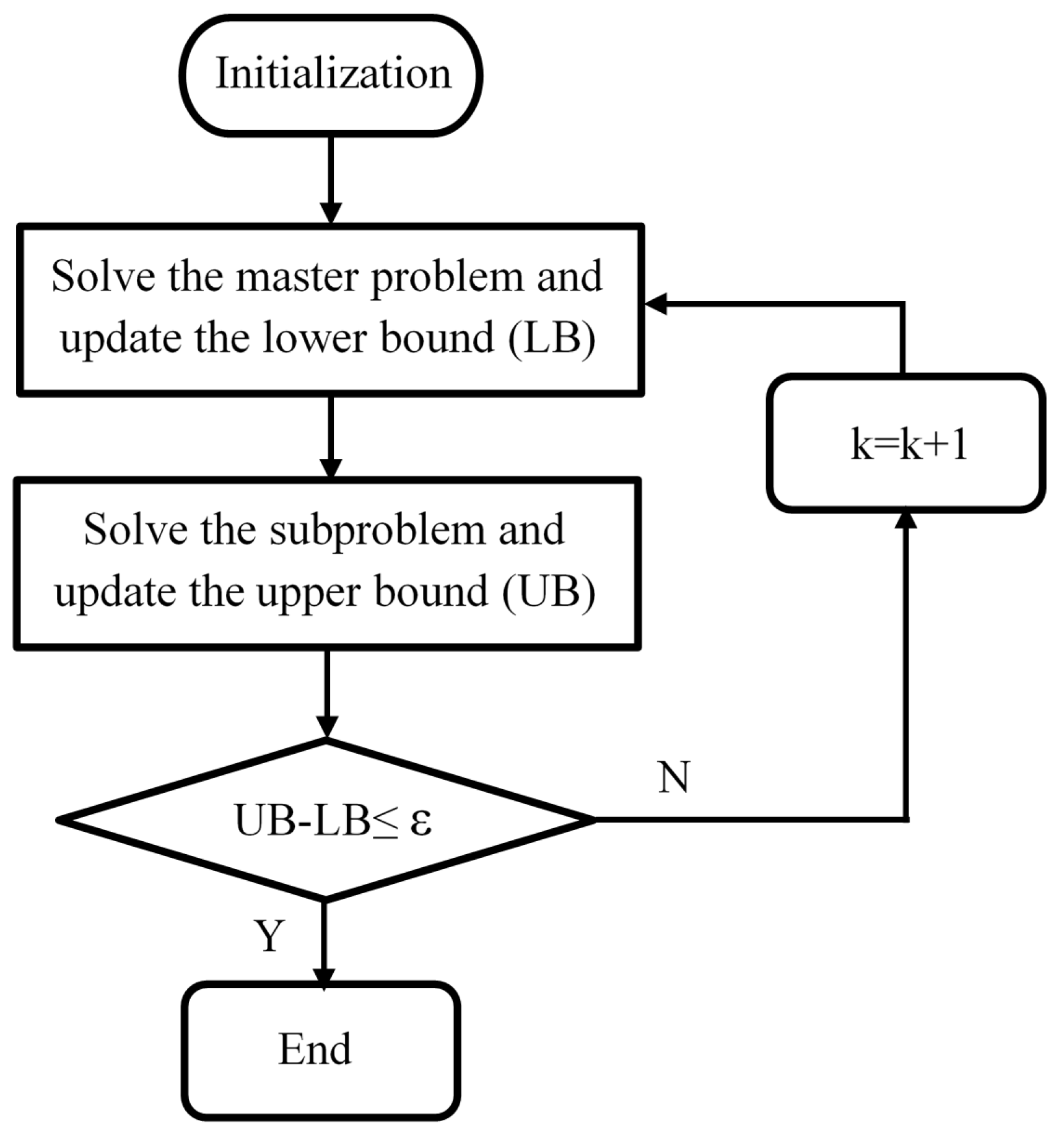
3.2. Solution Algorithm

The proposed tri-level “min-max-min” model in (2)–(12) is presented in a compact matrix form as in (13) to (14).

$$\underset{\mathbf{u}\in \mathbb{U}}{\min }\left\{A_0^{\mathrm{T}}\mathrm{u}+\underset{\mathbf{w}\in \mathbb{W}}{\max }\underset{\mathbf{x}\in \mathbb{X}\left(\mathbf{u},\mathbf{w}\right)}{\min }{B}_0^{\mathrm{T}}\mathbf{w}+C_0^{\mathrm{T}}\mathbf{x}\right\}$$

(13)

$$\begin{array}{ccc}\hfill \mathbb{X}\left(\mathbf{u},\mathbf{w}\right)& =& \left\{\mathbf{x}:A_1^{\mathrm{T}}\mathrm{u}+B_1^{\mathrm{T}}\mathbf{w}+C_1^{\mathrm{T}}\mathbf{x}={\mathbf{q}}_1,\right.\hfill \\ & & \left.A_2^{\mathrm{T}}\mathrm{u}+B_2^{\mathrm{T}}\mathbf{w}+C_2^{\mathrm{T}}\mathbf{x}\le {\mathbf{q}}_2;\right\}\hfill \end{array}$$

(14)

Note that the three optimization levels are nested together. To solve this problem, the C&CG algorithm and Benders decomposition algorithm have been investigated in [33] and [34], separately. The C&CG algorithm is employed to solve the proposed robust optimization in this work due to proven fast convergence [33]. First of all, according to the Karush-Kuhn-Tucker (KKT) conditions, the innermost “min” optimization is reformulated as complementary constraints. Since this problem is linear, strong duality holds. The inner “max-min” problem becomes a “max” problem. By Big-M method [35], the complementary constraints could be equivalently transformed into mixed-integer linear form. By this method, the original tri-level “min-max-min” problem is transformed into a bi-level “min-max” problem.

In the C&CG algorithm, the bi-level “min-max” problem is decomposed into a “min” master problem which optimizes the first- and second-stage decisions based on an increasing set of worst-case scenarios identified by the subproblems, and a “max” subproblem which determines the worst scenario based on the first-stage decisions determined by the master problem. The master problem generates a lower bound (LB) for the bi-level optimization problem since the set of worst scenarios are partial enumerations of the uncertainty region $\mathbb{W}$, while the subproblem problem generates an upper bound (UB) for the bi-level optimization problem since the first-stage decisions determined by the master problem are partial enumerations of $\mathbb{U}$. The master problem and subproblem are solved iteratively to narrow the gap between the upper and lower bounds until convergence. A simplified flow chart of the solution process is presented in Figure 2. Please refer to [33] for more details about the C&CG algorithm.

4. Case Studies

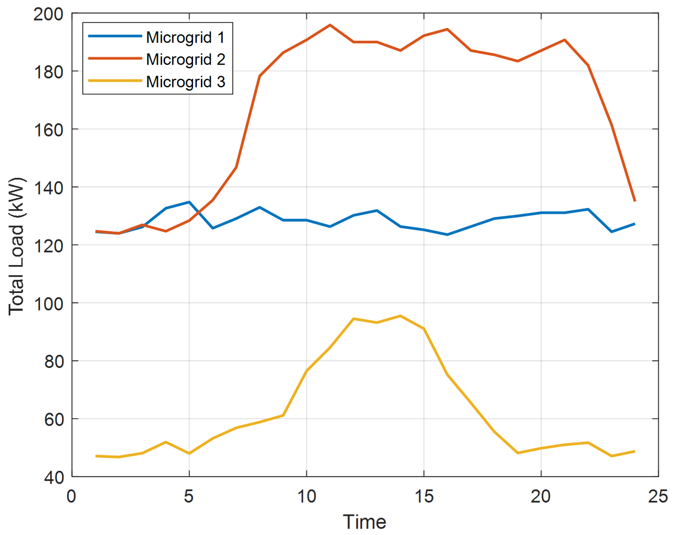
4.1. Test System Data

The proposed model for networked microgrids scheduling considering the stochastic unintentional islanding conditions was demonstrated using a modified Oak Ridge National Laboratory (ORNL) Distributed Energy Control and Communication (DECC) networked microgrids test system [36]. This system is consisted of three microgrids. Each microgrid includes one or multiple dispatchable DGs, undispatchable DGs (i.e., wind turbine and/or PV panel), and a battery, as shown in Figure 3.

The parameters of dispatchable DGs are listed in

Table 1. Dispatchable DG parameters.

DG Type	${\mathbf{P}}^{\mathbf{min}}$ (kW)	${\mathbf{P}}^{\mathbf{max}}$ (kW)	Start-Up Cost ($)	Shut-Down Cost ($)	Variable O&M Cost ($/kWh)	Fixed O&M Cost ($/h)
Diesel 1	20	60	3.5	1.75	0.3502	1
Diesel 2	20	60	3	1.5	0.5239	1
Diesel 3	20	60	2.5	1.25	0.6317	1
Microturbine 1	10	30	2	1	0.2885	1
Microturbine 2	10	30	2	1	0.4507	1
Microturbine 3	10	30	1.5	0.75	0.3885	1
Fuel Cell	10	30	1	0.5	0.3385	1

. The parameters of the battery are listed in

Table 2. Battery parameters.

Battery Type	Power Capacity (kW)	Energy Capacity (kWh)	${\mathrm{SOC}}^{\max }$ (%)	${\mathrm{SOC}}^{\min }$ (%)
Lithium-Ion	50	100	95	25
Degradation Cost ($/kWh)	Charging Efficiency (%)	Discharging Efficiency (%)	Initial SOC (%)	End SOC (%)
0.02	0.95	0.95	50	50

. Without loss of generality, the three batteries are assumed to have the same capacity and parameters. Note that these DGs and batteries are the dispatchable resources in the microgrid.

A wind turbine with 60 kW rated capacity is installed in microgrid 1 and 2, respectively. The wind power forecasted for the next 24-h scheduling horizon is listed in

Table 3. Forecasted wind power.

Hour	$\widehat{{\mathbf{P}}^{\mathbf{W}}}$ (kW)	Hour	$\widehat{{\mathbf{P}}^{\mathbf{W}}}$ (kW)	Hour	$\widehat{{\mathbf{P}}^{\mathbf{W}}}$ (kW)
1	51.4829	9	21.7503	17	24.2732
2	38.3711	10	34.8202	18	26.2555
3	43.5590	11	27.1748	19	26.7732
4	40.7514	12	30.1965	20	26.2159
5	27.7421	13	23.5169	21	32.8428
6	30.1540	14	39.4794	22	36.0156
7	28.6452	15	35.738	23	37.2312
8	23.3767	16	18.0583	24	44.1215

. The forecast error of wind power is assumed as ±35%. Microgrid 2 and 3 also have 50 kW PV panels installed separately. Similarly, the PV power forecasted for the next 24-h scheduling horizon is listed in

Table 4. Forecasted PV power.

Hour	${\mathbf{P}}^{\hat{\mathbf{P}}\mathbf{V}}$ (kW)	Hour	${\mathbf{P}}^{\hat{\mathbf{P}}\mathbf{V}}$ (kW)	Hour	${\mathbf{P}}^{\hat{\mathbf{P}}\mathbf{V}}$ (kW)
1	0	9	5.2978	17	14.1823
2	0	10	11.6044	18	4.6705
3	0	11	36.6382	19	0.1836
4	0	12	42.6778	20	0
5	0	13	35.2199	21	0
6	0	14	35.4594	22	0
7	0.1617	15	34.8303	23	0
8	1.7726	16	23.6244	24	0

. The forecast error of PV power is also assumed as ±35%. Due to geographical adjacency, the wind and PV power between microgrids are assumed to be perfect positive correlated.

The loads of the three microgrids are forecasted as in Figure 4. For each microgrid, these forecasted values are equally divided into two loads (one critical load and one non-critical load). Without loss of generality, a direct load control program is used as the demand response program. The customers simply get paid for their curtailment based on a linear penalty cost, i.e., value of lost load (VOLL). The VOLL is set as 2 $/kWh for the critical load and 1.5 $/kWh for the non-critical load, separately. This will guarantee the non-critical load gets curtailed before the critical load. The maximum percentage of allowed shedding for both loads is set as 80%. The forecast errors of both loads are assumed as ±9%.

The forecasted hourly utility rates are listed in

Table 5. Forecasted utility rates.

Hour	${\mathit{\lambda }}^{\mathbf{PCC}}$ (ct/kWh)	Hour	${\mathit{\lambda }}^{\mathbf{PCC}}$ (ct/kWh)	Hour	${\mathit{\lambda }}^{\mathbf{PCC}}$ (ct/kWh)
1	8.65	9	12.0	17	16.42
2	8.11	10	9.19	18	9.83
3	8.25	11	12.3	19	8.63
4	8.10	12	20.7	20	8.87
5	8.14	13	26.82	21	8.35
6	8.13	14	27.35	22	16.44
7	8.34	15	13.81	23	16.19
8	9.35	16	17.31	24	8.87

. It is assumed that the three microgrids have the same utility rates. For simplicity, the forecast errors of utility rates have been neglected. The maximum power at PCC is set as 200 kW for each microgrid.

The scheduling horizon is assumed for one day, i.e., 24 h, with hourly time intervals. The optimization model is programmed in MATLAB and solved by the mixed-integer linear programming (MILP) solver CPLEX 12.6 [37]. By setting the maximum allowed gap between the upper and lower bounds as 0.1, it generally takes less than 10 iterations for the C&CG algorithm to converge.

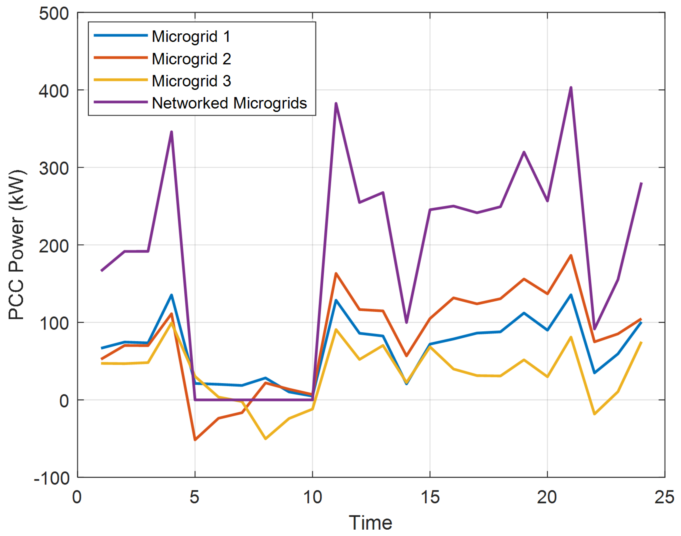
4.2. Advantages of Networked Microgrids

For simplicity, the robust control parameter for the unintentional islanding condition is normalized as ${\gamma }^{\mathrm{IS}}={\Gamma }^{\mathrm{IS}}/N_T$. Thus, ${\gamma }^{\mathrm{IS}}=0$ means no unintentional islanding is allowed and ${\gamma }^{\mathrm{IS}}=1$ means the networked microgrids are islanded all the time. Similarly, we normalized the robust control parameter for renewable generation and load as ${\gamma }_m^P={\Gamma }_{mt}^{\mathrm{P}}/\left(N_{mW}+N_{mPV}+N_{mD}\right)$ and assumed ${\gamma }_m^P$ is consistent for all microgrids and all time intervals. Therefore, ${\gamma }_m^P=0$ indicates that no uncertainties of renewable generation and load are considered. On the contrary, ${\gamma }_m^P=1$ means all uncertainties of renewable generation and load are considered, i.e., the solution is robust to all uncertainties.

To demonstrate the advantages of networked microgrids over independent microgrids, setting ${\gamma }_m^P=0.5$, the total operating cost and amount of load shedding for networked microgrids and independent microgrids under various values of ${\gamma }^{\mathrm{IS}}$ are calculated separately. The results are compared in Figure 5. First, when ${\gamma }^{\mathrm{IS}}$ increases, more loads are served by DGs to mitigate the impact of lost PCC power in case of unintentional islanding. Thus, the total cost increases, i.e., the resilience of microgrids is improved at the cost of increased operating cost. If committed DGs and ESSs are not sufficient, certain loads are shed as the last resort, as shown in Figure 5b. This holds for both networked microgrids and independent microgrids. Second, compared with independent microgrids, both the total operating cost and amount of load shedding of the networked microgrids are significantly reduced when ${\gamma }^{\mathrm{IS}}>0$, i.e., unintentional islanding happens. This result verifies the advantages of networked microgrids over independent microgrids in terms of both economics and resilience under the worst-case scenarios.

4.3. Convergence of C&CG Algorithm

To investigate the solution efficiency of the C&CG algorithm in large and networked microgrids, the total number of iterations needed for convergence of the C&CG algorithm under the cases of both independent microgrids and networked microgrids are compared in Figure 6. As can be seen, the C&CG algorithm converges in less than 10 iterations for all cases. In particular, the number of iterations needed for convergence of the C&CG algorithm does not increase as the number of microgrids is tripled, i.e., the solution efficiency of the C&CG algorithm is robust to the number of microgrids in the system.

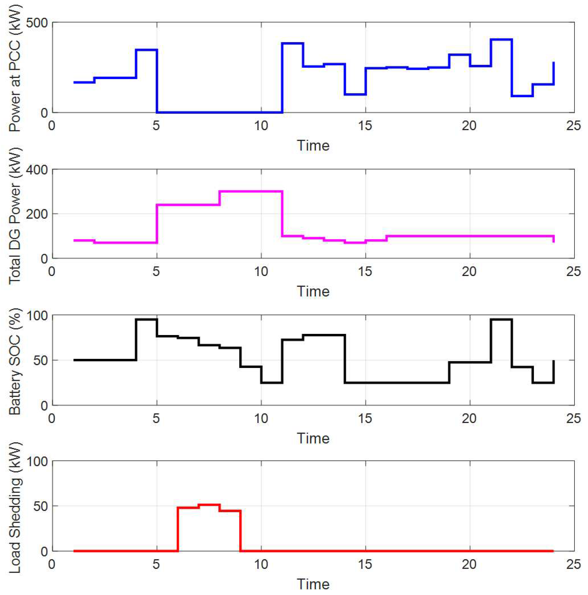
4.4. Example Solutions of C&CG Algorithm

The robust optimal dispatch of networked microgrids and the worst scenario of unintentional islanding condition when ${\gamma }^{\mathrm{IS}}=0.25$ and ${\gamma }^{\mathrm{P}}=0.5$ are shown in Figure 7. As can be seen, in the worst scenario, the networked microgrids are islanded from hour 5 to hour 10, i.e., the PCC power is forced to be 0 during these 6 h. To get prepared for this islanding situation, the ESSs are charged to their maximum SOC (i.e., 95%) before islanding. Once the islanding happens, the PCC power is instantaneously forced to be 0. The ESSs start to discharge to mitigate the losing power at PCC. Meanwhile, the DGs also increase their power outputs. By the end of the islanding time periods, the ESSs have been discharged to their minimum SOC (i.e., 25%). As a result, load shedding is still performed during certain hours. The total PCC power, total output power of DGs, total battery SOC, and load shedding decisions are shown in Figure 7.

To show the coordination between microgrids, especially during the islanded time periods, the PCC power of each microgrid and the total PCC power of networked microgrids are compared in Figure 8. As can be seen, all three microgrids import power from the utility grid when they are grid-connected. When islanded during hours 5–10, microgrid 1 imports power from both microgrid 2 and microgrid 3. Nevertheless, the total PCC power of networked microgrids remains at 0 during the islanded time periods. During hours 5–7, microgrid 2 is lightly loaded as shown in Figure 4. Thus, power is exported from microgrid 2 to microgrids 1 and 3. However, the load of microgrid 2 increases rapidly during hours 8–10. Under this situation, microgrid 3 starts to export power to microgrids 1 and 2. Due to these kinds of interactions between microgrids, both the total operating cost and the amount of load shedding of the networked microgrids are significantly reduced.

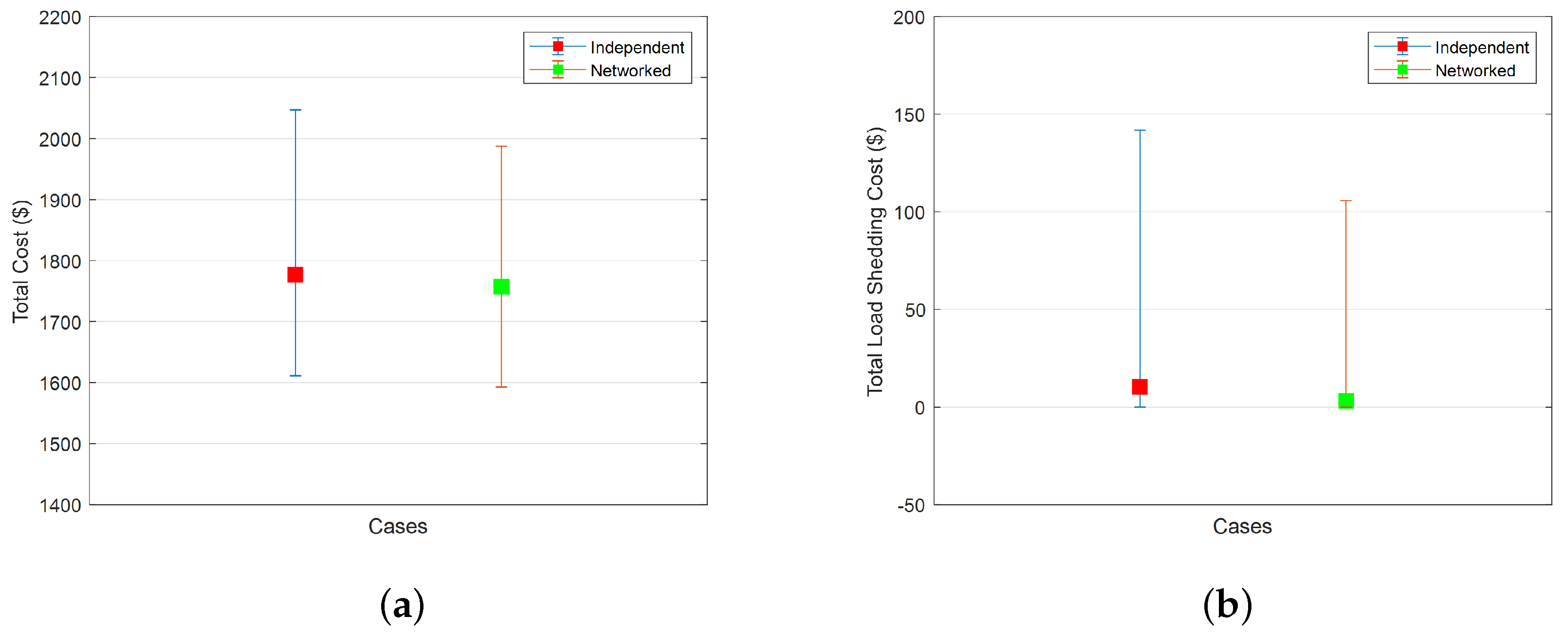
4.5. Stochastic Evaluation of Independent Microgrids and Networked Microgrids

In this subsection, the results of robust optimization for independent microgrids and networked microgrids are evaluated and compared. For this purpose, $P_{wt}^{\mathrm{W}}$, $P_{vt}^{\mathrm{PV}}$, $P_{dt}^{\mathrm{L}}$, and $Z_t^{\mathrm{G}}$ are modeled as random variables with known probability distribution functions, based on which a test set of 1000 scenarios is constructed through Monte Carlo simulation. Traditionally, load $P_{dt}^{\mathrm{L}}$ could be modeled as a Gaussian distribution [38]. Wind power $P_{wt}^{\mathrm{W}}$ is modeled as a Gaussian distribution or Weibull distribution [39]. PV output $P_{vt}^{\mathrm{PV}}$ is modeled as a Gaussian distribution or $\beta$ distribution [40]. In each scenario, the loads are assumed to have a Gaussian distribution with mean $P_{mdt}^{\hat{\mathrm{L}}}$ and standard deviation ${\delta }_{mdt}^{\mathrm{L}}/3$. The PV and wind power are also assumed to have a Gaussian distribution with mean $P_{mvt}^{\hat{\mathrm{P}}\mathrm{V}}$ and $P_{mvt}^{\hat{\mathrm{W}}}$, and standard deviation ${\delta }_{mvt}^{\mathrm{PV}}$ and ${\delta }_{mvt}^{\mathrm{W}}$, separately. The occurrence time of unintentional islanding is assumed to have a uniform distribution along the scheduling horizon. Once the occurrence time is determined, the duration of the unintentional islanding is assumed as a uniform distribution between 1 and the uncertainty budget ${\Gamma }^{\mathrm{IS}}$.

In the first case, we set ${\gamma }^{\mathrm{IS}}=0.25$ and ${\gamma }^{\mathrm{P}}=0.5$; i.e., the uncertainty budget of unintentional islanding condition is set as ${\gamma }^{\mathrm{IS}}\times N_T=6$ h. Then, the robust optimization model is solved for independent microgrids and networked microgrids, separately. Next, for each test scenario, the first stage decisions, i.e., the commitment status of DGs, of both independent microgrids and networked microgrids are evaluated. The step-by-step procedures of this study are summarized as follows:

Step 1:

Set the uncertainty budget of unintentional islanding condition ${\gamma }^{\mathrm{IS}}$ and uncertainty budget of renewable generation and load ${\gamma }^{\mathrm{P}}$.

Step 2:

Solve the robust optimization model for networked microgrids and each independent microgrid separately.

Step 3:

Generate the test set of 1000 scenarios.

Step 4:

For networked microgrids, fix the commitment status of DGs and conduct Monte Carlo simulation for each test scenario.

Step 5:

For each independent microgrid, fix the commitment status of DGs and conduct Monte Carlo simulation for each test scenario.

Step 6:

Collect the total operating costs and load shedding costs for further comparison and analysis.

The total operating cost and load shedding cost are collected and compared in Figure 9. The minimum, maximum, and average value of the total operating cost of independent microgrids and networked microgrids are compared and shown in Figure 9a. As can be seen, the networked microgrids outperform independent microgrids in terms of both average cost and the total cost in the worst scenario. The minimum, maximum, and average value of the load shedding cost of independent microgrids and networked microgrids are compared and shown in Figure 9b. As can be seen, the networked microgrids outperform independent microgrids in terms of both the average load shedding cost and the load shedding cost in the worst scenario.

In the second case, we set ${\gamma }^{\mathrm{IS}}=0.5$ and ${\gamma }^{\mathrm{P}}=0.5$, i.e., the uncertainty budget of the unintentional islanding condition is set as ${\gamma }^{\mathrm{IS}}\times N_T=12$ hours. Similarly, a test set of 1000 scenarios is constructed through Monte Carlo simulation. Then, the robust optimization model is solved for independent microgrids and networked microgrids, separately. Next, for each test scenario, the first stage decisions, i.e., the commitment status of DGs, of both independent microgrids and networked microgrids are evaluated. The total operating cost and load shedding cost are collected and compared in Figure 10. The minimum, maximum, and average value of the total operating cost of independent microgrids and networked microgrids are compared and shown in Figure 10a. As can be seen, the total operating costs of both independent microgrids and networked microgrids increase as longer islanding durations are considered. Nevertheless, networked microgrids outperform independent microgrids significantly in terms of both average cost and the total cost in the worst scenario. The minimum, maximum, and average value of the load shedding cost of independent microgrids and networked microgrids are compared and shown in Figure 10b. As can be seen, both load shedding costs increase as longer islanding durations are considered. Still, networked microgrids outperform independent microgrids in terms of both the average load shedding cost and the load shedding cost in the worst scenario.

It should be noted that the optimality of the solution obtained by the robust optimization cannot be guaranteed. In fact, the robust optimization tends to take a conservative action to handle the modeled uncertainties by turning on more DGs. Thus, stochastic optimization usually outperforms robust optimization in terms of average cost. However, stochastic optimization is subject to incur huge costs in high-impact, low-probability (HILP) scenarios. In contrast, robust optimization is designed to optimize the cost in the worst scenario and thus can significantly improve the system performance in HILP scenarios, i.e., improve the system resilience. In other words, robust optimization tends to sacrifice certain optimality for resilience. Nevertheless, with properly chosen robust control parameters, the solution obtained by robust optimization can ensure both resilience and near-optimality. By the central limit theorem, when a large number (N) of independent random variables are aggregated, the volatility scales according to $O\left(\sqrt{N}\right)$. Therefore, a proper level of the normalized robust control parameter should be chosen close to $O\left(\sqrt{N}\right)/N$ [34]. An advanced approach, which reduces conservativeness by removing the ineffective parts of the uncertainty set, was recently proposed in [41].

5. Conclusions

In this paper, a two-stage adaptive robust optimization model is proposed for networked microgrid scheduling considering the stochastic unintentional islanding conditions and conventional forecast errors of both renewable generation and loads. By coordinating the dispatch of DERs and responsive demand among multiple networked microgrids, the total cost, including the operating cost of DERs, the cost of trading power with the utility grid, and the cost associated with load shedding, is minimized. The C&CG algorithm has been employed to solve the proposed optimization problem efficiently.

The correctness and effectiveness of the proposed approach was demonstrated through case studies on a modified ORNL DECC networked microgrid test system, consisting of three microgrids. Compared with the results of independent microgrids, it has been proven that both the total operating cost and the amount of load shedding of networked microgrids are significantly reduced when ${\gamma }^{\mathrm{IS}}>0$, i.e., unintentional islanding happens. In the worst scenario, the total cost could be reduced more than 10%. Meanwhile, the amount of load shedding could be reduced to 15%. In addition, results of Monte Carlo simulation verified that networked microgrids outperformed independent microgrids significantly in terms of both average cost and average load shedding.

It has also been approved that the solution efficiency of the C&CG algorithm is robust to the number of microgrids in the system. Future works include expanding the islanding capability from a simple power balance constraint to a power flow constraint and dynamic stability constraint. In addition, distributed optimization algorithms, which could preserve the privacy of customers and enable plug-and-play of microgrids, will be investigated.

References

1. Cagnano, A.; De Tuglie, E.; Mancarella, P. Microgrids: Overview and guidelines for practical implementations and operation. Appl. Energy 2020, 258, 114039. [Google Scholar] [CrossRef]
2. Khan, M.Z.; Mu, C.; Habib, S.; Alhosaini, W.; Ahmed, E.M. An Enhanced Distributed Voltage Regulation Scheme for Radial Feeder in Islanded Microgrid. Energies 2021, 14, 6092. [Google Scholar] [CrossRef]
3. Park, B.; Zhang, Y.; Olama, M.; Kuruganti, T. Model-free control for frequency response support inmicrogrids utilizing wind turbines. Elec. Power Syst. Res. 2021, 194, 107080. [Google Scholar] [CrossRef]
4. Liu, R.; Wang, S.; Liu, G.; Wen, S.; Zhang, J.; Ma, Y. An Improved Virtual Inertia Control Strategy for Low Voltage AC Microgrids with Hybrid Energy Storage Systems. Energies 2022, 15, 442. [Google Scholar] [CrossRef]
5. Wang, Y.; Rousis, A.O.; Strbac, G. On microgrids and resilience: A comprehensive review on modeling and operational strategies. Renew. Sustain. Energy Rev. 2020, 134, 110313. [Google Scholar] [CrossRef]
6. Warneryd, M.; Hakansson, M.; Karltorp, K. Unpacking the complexity of community microgrids: A review of institutions’ roles for development of microgrids. Renew. Renew. Sustain. Energy Rev. 2020, 121, 109690. [Google Scholar] [CrossRef]
7. Chen, B.; Wang, J.; Lu, X.; Chen, C.; Zhao, S. Networked Microgrids for Grid Resilience, Robustness, and Efficiency: A Review. IEEE Trans. Smart Grid 2021, 12, 18–32. [Google Scholar] [CrossRef]
8. Wang, L.; Zhu, Z.; Jiang, C.; Li, Z. Bi-Level Robust Optimization for Distribution System With Multiple Microgrids Considering Uncertainty Distribution Locational Marginal Price. IEEE Trans. Smart Grid 2021, 12, 1104–1117. [Google Scholar] [CrossRef]
9. Hussain, A.; Bui, V.H.; Kim, H.M. A Resilient and Privacy- Preserving Energy Management Strategy for Networked Microgrids. IEEE Trans. Smart Grid 2018, 9, 2127–2139. [Google Scholar] [CrossRef]
10. Li, Z.; Shahidehpour, M. Privacy-Preserving Collaborative Operation of Networked Microgrids with the Local Utility Grid Based on Enhanced Benders Decomposition. IEEE Trans. Smart Grid 2020, 11, 2638–2651. [Google Scholar] [CrossRef]
11. Xu, Q.; Zhao, T.; Xu, Y.; Xu, Z.; Wang, P.; Blaabjerg, F. A Distributed and Robust Energy Management System for Networked Hybrid AC/DC Microgrids. IEEE Trans. Smart Grid 2020, 11, 3496–3508. [Google Scholar] [CrossRef]
12. Bajwa, A.A.; Mokhlis, H.; Mekhilef, S.; Mubin, M. Enhancing power system resilience leveraging microgrids: A review. J. Renew. Sustain. Energy 2019, 11, 035503. [Google Scholar] [CrossRef]
13. Liu, G.; Jiang, T.; Ollis, T.B.; Li, X.; Li, F.; Tomsovic, K. Resilient distribution system leveraging distributed generation and microgrids: A review. IET Energy Syst. Integr. 2020, 2, 289–304. [Google Scholar] [CrossRef]
14. Xu, Y.; Liu, C.C.; Schneider, K.P.; Tuffner, F.K.; Ton, D. Microgrids for Service Restoration to Critical Load in a Resilient Distribution System. IEEE Trans. Smart Grid 2018, 9, 426–437. [Google Scholar] [CrossRef]
15. Arif, A.; Wang, Z. Networked microgrids for service restoration in resilient distribution systems. IET Gener. Transm. Distrib. 2017, 11, 3612–3619. [Google Scholar] [CrossRef]
16. Lin, W.; Zhu, J.; Yuan, Y.; Wu, H. Robust Optimization for Island Partition of Distribution System Considering Load Forecasting Error. IEEE Access 2019, 7, 64247–64255. [Google Scholar] [CrossRef]
17. Zhou, Q.; Shahidehpour, M.; Alabdulwahab, A.; Abusorrah, A. Flexible Division and Unification Control Strategies for Resilience Enhancement in Networked Microgrids. IEEE Trans. Power Syst. 2020, 35, 474–486. [Google Scholar] [CrossRef]
18. Marchgraber, J.; Gawlik, W. Investigation of Black-Starting and Islanding Capabilities of a Battery Energy Storage System Supplying a Microgrid Consisting of Wind Turbines, Impedance- and Motor-Loads. Energies 2020, 13, 5170. [Google Scholar] [CrossRef]
19. Zhao, Y.; Lin, Z.; Ding, Y.; Liu, Y.; Sun, L.; Yan, Y. A Model Predictive Control Based Generator Start-Up Optimization Strategy for Restoration With Microgrids as Black-Start Resources. IEEE Trans. Power Syst. 2018, 33, 7189–7203. [Google Scholar] [CrossRef]
20. Francisco, F.; Giraldez, J.; Pratt, A. Networked Microgrid Optimal Design and Operations Tool: Regulatory and Business Environment Study; NREL/TP-5D00-70944; National Renewable Energy Laboratory: Golden, CO, USA, 2020. [Google Scholar]
21. Liu, G.; Starke, M.; Xiao, B.; Zhang, X.; Tomsovic, K. Microgrid Optimal Scheduling With Chance-Constrained Islanding Capability. Electr. Power Syst. Res. 2017, 145, 197–206. [Google Scholar] [CrossRef] [Green Version]
22. Hemmati, M.; Mohammadi-Ivatloo, B.; Abapour, M.; Anvari-Moghaddam, A. Optimal Chance-Constrained Scheduling of Reconfigurable Microgrids Considering Islanding Operation Constraints. IEEE Syst. J. 2020, 14, 5340–5349. [Google Scholar] [CrossRef]
23. Farzin, H.; Fotuhi-Firuzabad, M.; Moeini-Aghtaie, M. Stochastic Energy Management of Microgrids During Unscheduled Islanding Period. IEEE Trans. Ind. Inform. 2017, 13, 1079–1087. [Google Scholar] [CrossRef]
24. Liu, G.; Starke, M.; Xiao, B.; Tomsovic, K. Robust Optimization Based Microgrid Scheduling with Islanding Constraints. IET Gener. Transm. Distrib. 2017, 11, 1820–1828. [Google Scholar] [CrossRef]
25. Liu, G.; Ollis, T.B.; Zhang, Y.; Jiang, T.; Tomsovic, K. Robust Microgrid Scheduling With Resiliency Considerations. IEEE Access 2020, 8, 153169–153182. [Google Scholar] [CrossRef]
26. Kumari, K.S.K.; Babu, R.S.R. Optimal scheduling of a micro-grid with multi-period islanding constraints using hybrid CFCS technique. Evol. Intell. 2021, 15, 723–742. [Google Scholar] [CrossRef]
27. Guo, Y.; Zhao, C. Islanding-Aware Robust Energy Management for Microgrids. IEEE Trans. Smart Grid 2018, 9, 1301–1309. [Google Scholar] [CrossRef]
28. Shahid, F.; Zameer, A.; Muneeb, M. A novel genetic LSTM model for wind power forecast. Energy 2021, 223, 1200692. [Google Scholar] [CrossRef]
29. Mora, E.; Cifuentes, J.; Marulanda, G. Short-Term Forecasting of Wind Energy: A Comparison of Deep Learning Frameworks. Energies 2021, 14, 7943. [Google Scholar] [CrossRef]
30. Ahmed, R.; Sreeram, V.; Mishra, Y.; Arif, M.D. A review and evaluation of the state-of-the-art in PV solar power forecasting: Techniques and optimization. Renew. Sustain. Energy Rev. 2020, 124, 109792. [Google Scholar] [CrossRef]
31. Sundararajan, A.; Ollis, B. Regression and Generalized Additive Model to Enhance the Performance of Photovoltaic Power Ensemble Predictors. IEEE Access 2021, 9, 111899–111914. [Google Scholar] [CrossRef]
32. Ortega-Vazquez, M. Optimizing the Spinning Reserve Requirements; The University of Manchester: Manchester, UK, 2006; pp. 1–219. Available online: https://labs.ece.uw.edu/real/Library/Thesis/Miguel_ORTEGA-VAZQUEZ.pdf (accessed on 1 March 2022).
33. Zeng, B.; Zhao, L. Solving two-stage robust optimization problems using a column-and-constraint generation method. Oper. Res. Lett. 2013, 41, 457–461. [Google Scholar] [CrossRef]
34. Bertsimas, D.; Litvinov, E.; Sun, X.A.; Zhao, J.; Zheng, T. Adaptive robust optimization for the security constrained unit commitment problem. IEEE Trans. Power Syst. 2013, 28, 52–63. [Google Scholar] [CrossRef]
35. Jiang, R.; Wang, J.; Guan, Y. Robust Unit Commitment With Wind Power and Pumped Storage Hydro. IEEE Trans. Power Syst. 2012, 27, 800–810. [Google Scholar] [CrossRef]
36. Xiao, B.; Starke, M.; Liu, G.; Ollis, B.; Irminger, P.; Dimitrovski, A.; Prabakar, K.; Dowling, K.; Xu, Y. Development of hardware-in-the-loop microgrid testbed. In Proceedings of the 2015 IEEE Energy Conversion Congress and Exposition (ECCE), Montreal, QC, Canada, 20–24 September 2015; pp. 1196–1202. [Google Scholar]
37. The IBM ILOG CPLEX Optimization Studio. 2022. Available online: https://www.ibm.com/products/ilog-cplex-optimization-studio?utm_content=SRCWW&p1=Search&p4=43700050328194740&p5=e&gclid=Cj0KCQjw29CRBhCUARIsAOboZbI0ay13LpL9AR2CT7A-GWbanqyRRsSiBT7B1Hu1eyUWeB783GaIINYaAoWVEALw_wcB&gclsrc=aw.ds (accessed on 1 March 2022).
38. Liu, G.; Tomsovic, K. Robust Unit Commitment Considering Uncertain Demand Response. Electr. Power Syst. Res. 2015, 119, 126–137. [Google Scholar] [CrossRef] [Green Version]
39. Erdinc, F.G.; Cicek, A.; Erdinc, O.; Yumurtaci, R. Uncertainty-Aware Decision Making in Power Systems Including Energy Storage, Dynamic Line Rating and Responsive Demand as Multiple Flexibility Resources. In Proceedings of the 2021 International Conference on Smart Energy Systems and Technologies (SEST), Vaasa, Finland, 6–8 September 2021; pp. 1–6. [Google Scholar]
40. Wu, Y.K.; Lai, Y.H.; Huang, C.L.; Phuong, N.T.B.; Tan, W.S. Artificial Intelligence Applications in Estimating Invisible Solar Power Generation. Energies 2022, 15, 1312. [Google Scholar] [CrossRef]
41. Dehghani-Filabadi, M.; Mahmoudzadeh, H. Effective Budget of Uncertainty for Classes of Robust Optimization. INFORMS J. Optim. 2022. Available online: Https://pubsonline.informs.org/doi/10.1287/ijoo.2021.0069 (accessed on 1 March 2022).
Figure 1. Illustration of networked microgrids.
Energies 15 02249 g001
Figure 2. Solution process of the C&CG algorithm.
Energies 15 02249 g002
Figure 3. Modified ORNL DECC networked microgrids test system.
Energies 15 02249 g003
Figure 4. The total load of each microgrid.
Energies 15 02249 g004
Figure 5. Comparison of total operating cost and amount of load shedding between networked microgrids and independent microgrids under various values of γ IS . (a) Total operating cost. (b) Total load shedding.
Energies 15 02249 g005
Figure 6. Comparison of iterations needed for convergence of the C&CG algorithm between networked microgrids and independent microgrids under various values of γ IS .
Energies 15 02249 g006
Figure 7. Total PCC power, output power of DGs, total battery SOC, and load shedding decisions of networked microgrids under γ IS = 0.25 , γ P = 0.5 .
Energies 15 02249 g007
Figure 8. PCC power of individual microgrids and networked microgrids under γ IS = 0.25 , γ P = 0.5 .
Energies 15 02249 g008
Figure 9. Comparison of total operating cost and load shedding cost of independent and networked microgrids under γ IS = 0.25 and γ P = 0.5 . (a) Total operating cost. (b) Load shedding cost.
Energies 15 02249 g009
Figure 10. Comparison of total operating cost and load shedding cost of independent and networked microgrids under γ IS = 0.5 and γ P = 0.5 . (a) Total operating cost. (b) Load shedding cost.
Energies 15 02249 g010