
BiLSTM Network-Based Approach for Solar Irradiance Forecasting in Continental Climate Zones


Abstract
:1. Introduction
1.1. World PV Growth
1.2. Related Work
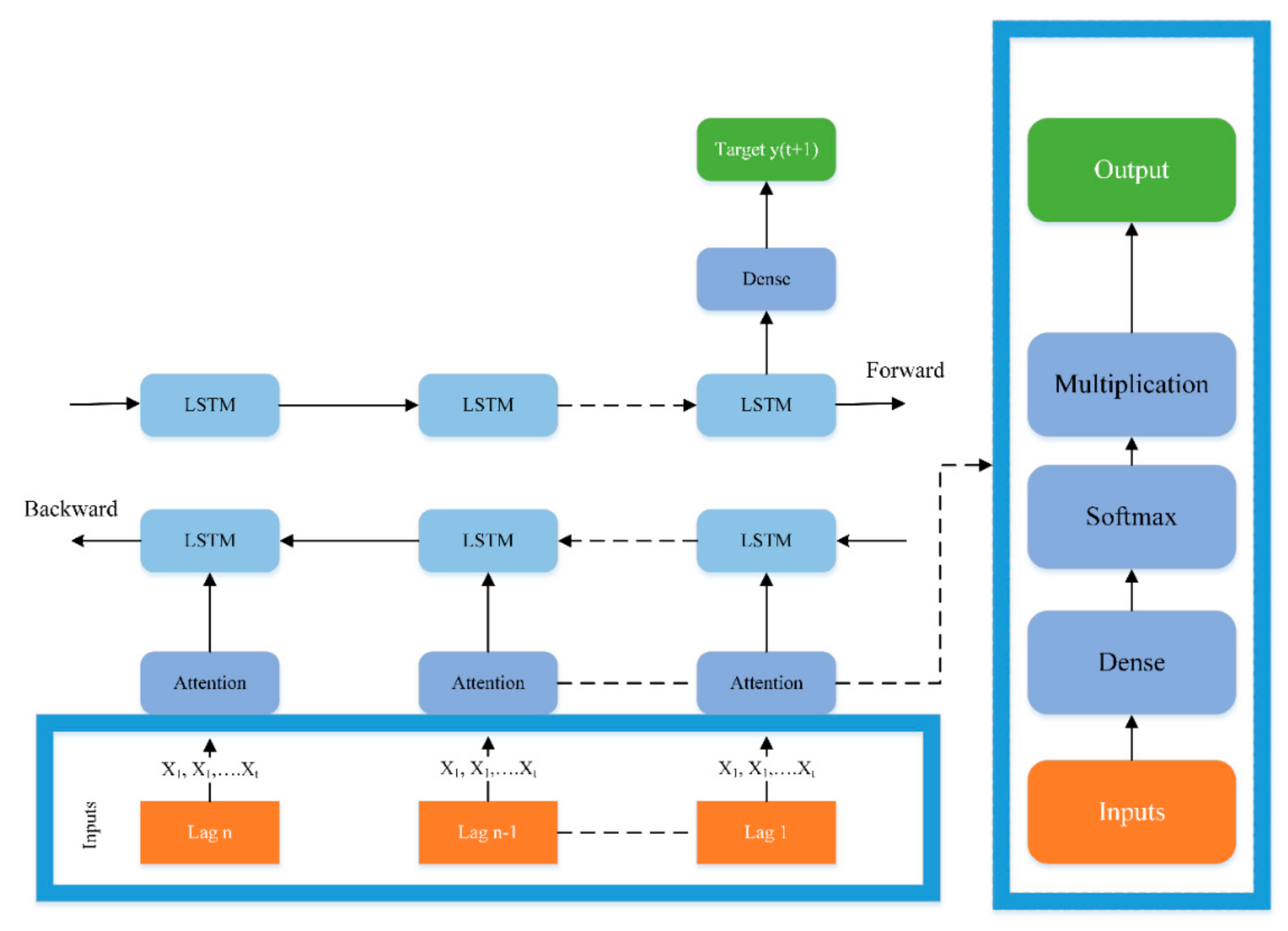
2. Attention-Based BILSTM
2.1. Encoder Layer
2.2. Layer of Attention
2.3. Softmax Layer
2.4. Training of Model
2.5. Metrics for Performance Evaluation
3. Results and Discussion
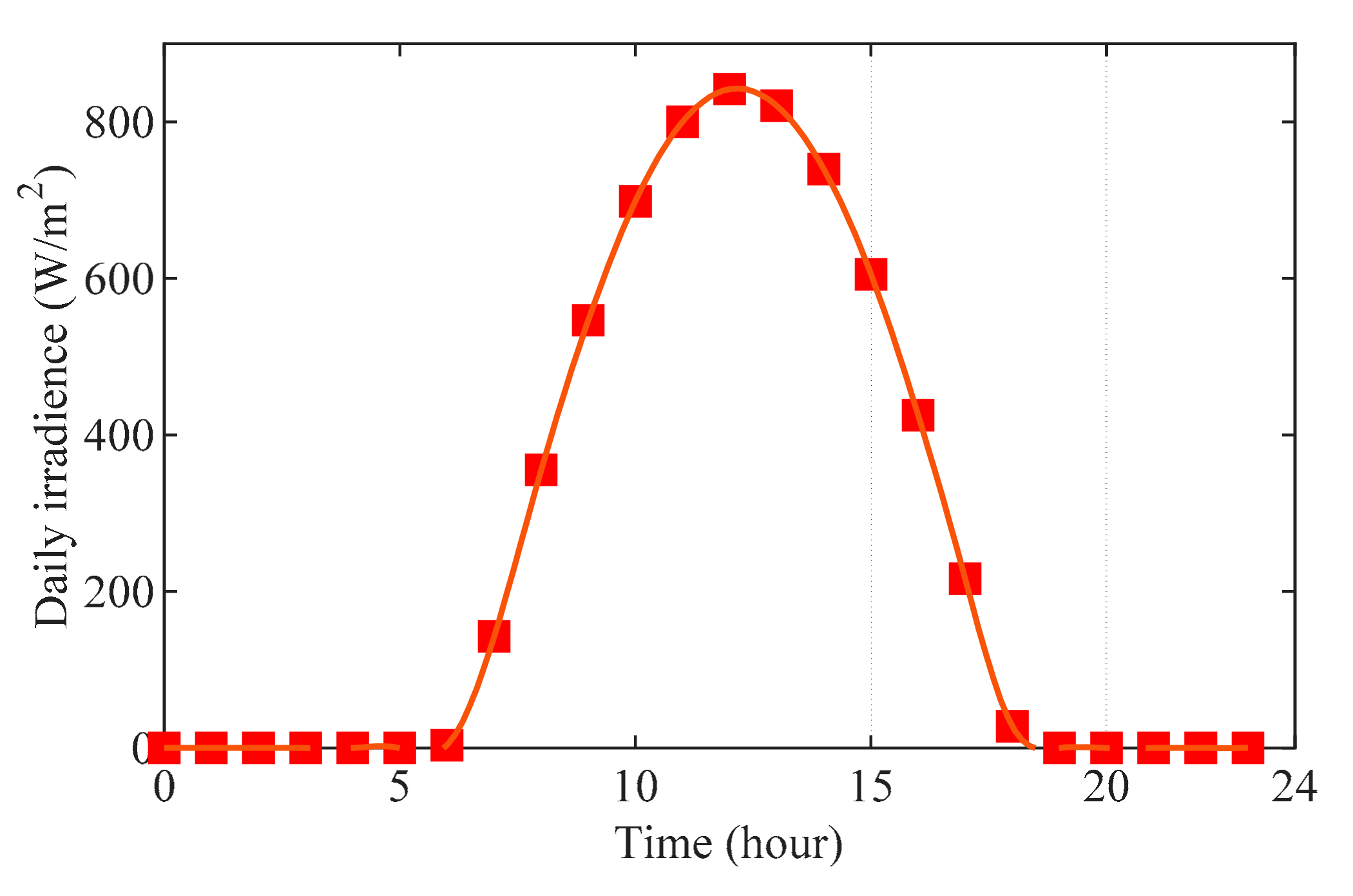
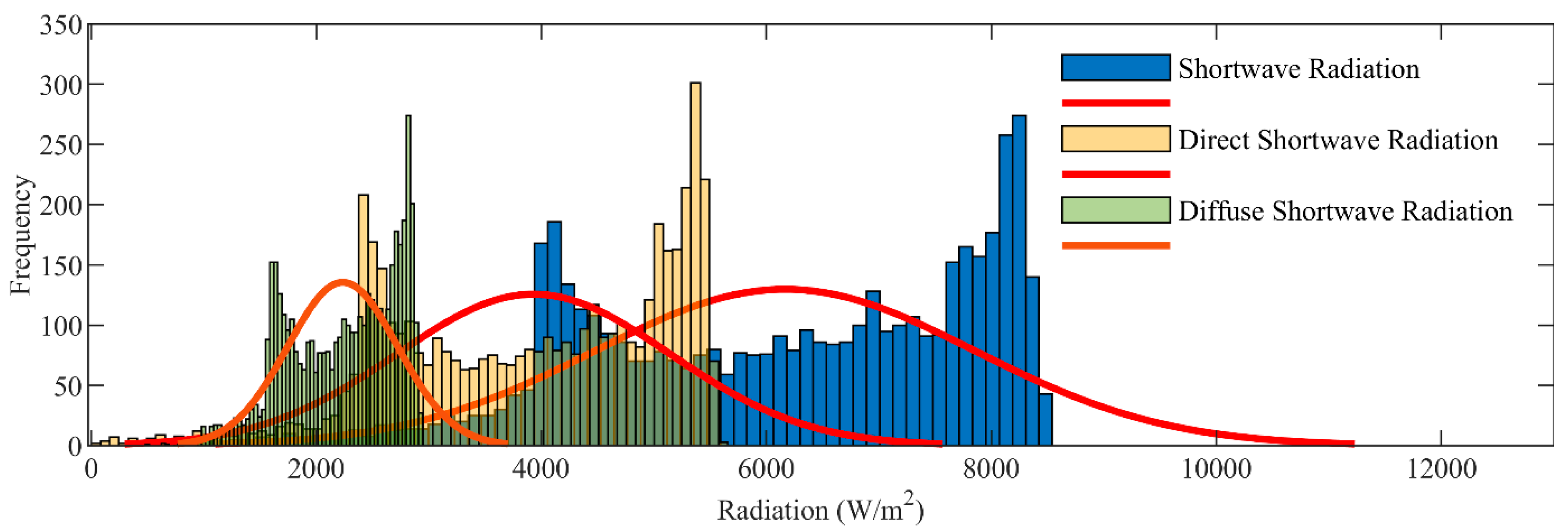
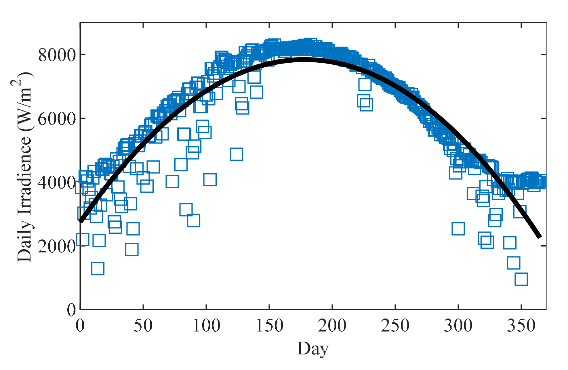
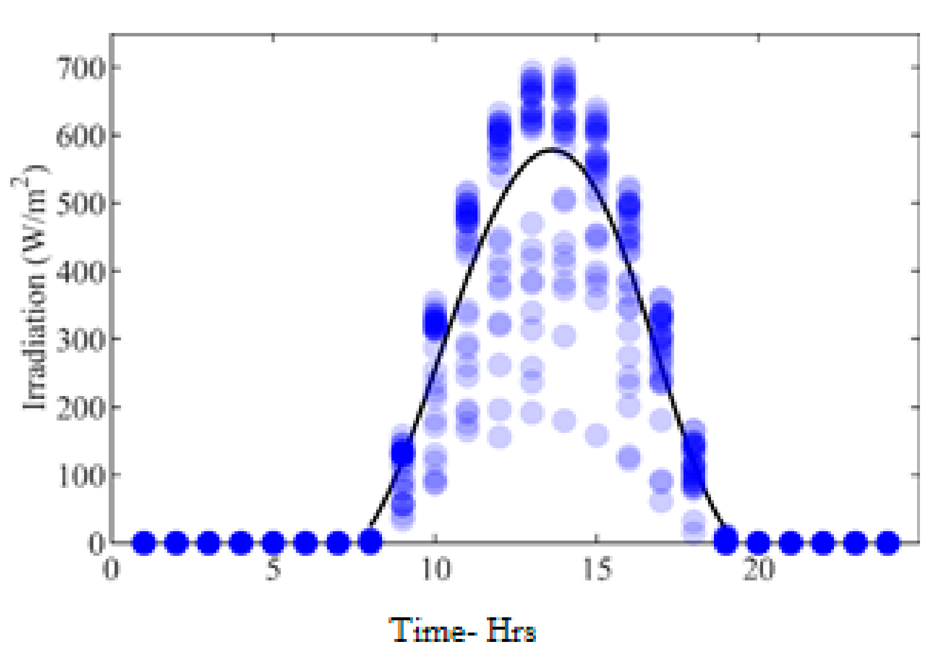
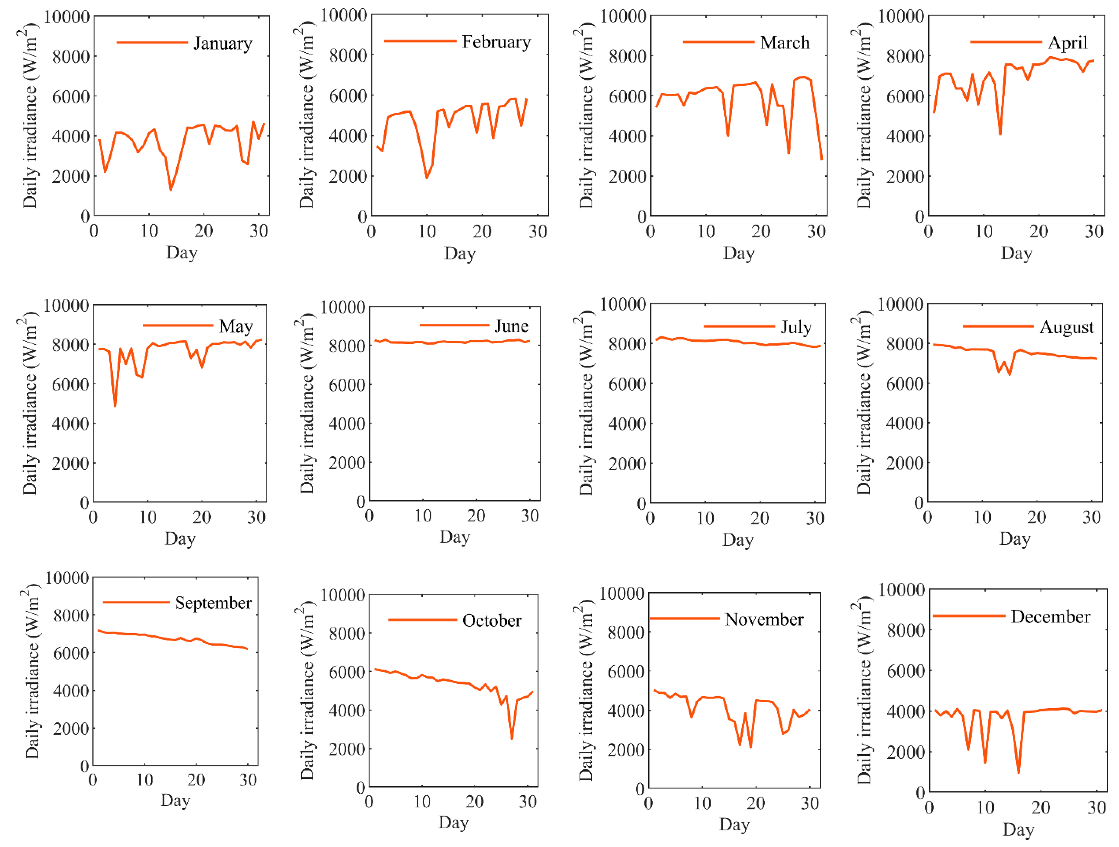
3.1. Data Analysis
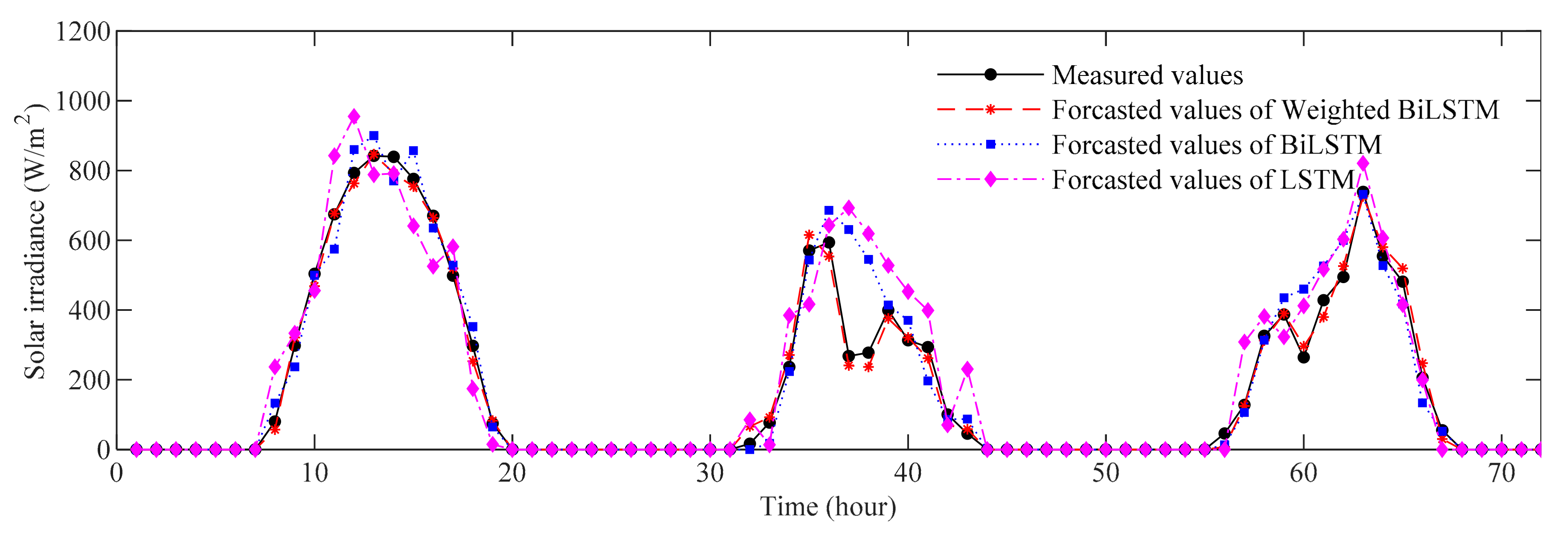
3.2. Results
4. Conclusions
Author Contributions
Funding
Institutional Review Board Statement
Informed Consent Statement
Conflicts of Interest
References
- Heng, J.; Wang, J.; Xiao, L.; Lu, H. Research and application of a combined model based on frequent pattern growth algorithm and multi-objective optimization for solar radiation forecasting. Appl. Energy 2017, 208, 845–866. [Google Scholar] [CrossRef]
- Amrouche, B.; Sicot, L.; Guessoum, A.; Belhamel, M. Experimental analysis of the maximum power point’s properties for four photovoltaic modules from different technologies: Monocrystalline and polycrystalline silicon, CIS and CdTe. Sol. Energy Mater. Sol. Cells 2013, 118, 124–134. [Google Scholar] [CrossRef]
- Lubitz, W.D. Effect of manual tilt adjustments on incident irradiance on fixed and tracking solar panels. Appl. Energy 2011, 88, 1710–1719. [Google Scholar] [CrossRef]
- Jung, S.; Yoon, Y.T. Optimal Operating Schedule for Energy Storage System: Focusing on Efficient Energy Management for Microgrid. Processes 2019, 7, 80. [Google Scholar] [CrossRef] [Green Version]
- International Energy Agency. 2020. Available online: https://www.iea.org/fuels-and-technologies/solar (accessed on 1 October 2020).
- Menacho, Á.H. Concentrated Solar Power Generation: Triple Bottom Line Assessment in Europe and China 2020–2050. 2020. Available online: http://resolver.tudelft.nl/uuid:272b700c-50b8-4767-b4f7-8694ea3c223b (accessed on 1 December 2020).
- Statista. Cumulative Installed Solar Power Capacity in China from 2012 to 2019. 2020. Available online: https://www.statista.com/statistics/279504/cumulative-installed-cpacity-of-solar-power-in-china/ (accessed on 1 October 2020).
- CleanTechnica. Chinese Solar Perseveres during Pandemic. 2020. Available online: https://cleantechnica.com/2020/05/21/chinese-solar-perseveres-during-pandemic/ (accessed on 1 October 2020).
- International Energy Agency. IEA: Global Installed PV Capacity Leaps to 303 Gigawatts. 2020. Available online: https://www.iea.org/reports/solar-pv (accessed on 1 October 2020).
- International Energy Agency. Solar PV. 2020. Available online: https://www.iea.org/reports/solar-pv (accessed on 1 October 2020).
- Box, G.E.P.; Jenkins, G.M.; Reinsel, G.C.; Ljung, G.M. Time Series Analysis: Forecasting and Control; John Wiley & Sons: Hoboken, NJ, USA, 2015. [Google Scholar]
- Mateo, F.; Carrasco, J.J.; Sellami, A.; Millán-Giraldo, M.; Domínguez, M.; Soria-Olivas, E. Machine learning methods to forecast temperature in buildings. Expert Syst. Appl. 2013, 40, 1061–1068. [Google Scholar] [CrossRef]
- Zhang, G.P. Time series forecasting using a hybrid ARIMA and neural network model. Neurocomputing 2003, 50, 159–175. [Google Scholar] [CrossRef]
- Li, Y.; Su, Y.; Shu, L. An ARMAX model for forecasting the power output of a grid-connected photovoltaic system. Renew. Energy 2014, 66, 78–89. [Google Scholar] [CrossRef]
- Kariniotakis, G. Renewable Energy Forecasting: From Models to Applications; Woodhead Publishing: Kidlington, UK, 2017. [Google Scholar]
- Brockwell, P.J.; Brockwell, P.J.; Davis, R.A.; Davis, R.A. Introduction to Time Series and Forecasting; Springer: Berlin/Heidelberg, Germany, 2016. [Google Scholar]
- Creal, D.; Koopman, S.J.; Lucas, A. Generalized autoregressive score models with applications. J. Appl. Econom. 2013, 28, 777–795. [Google Scholar] [CrossRef] [Green Version]
- Neves, C.; Fernandes, C.; Hoeltgebaum, H. Five different distributions for the Lee–Carter model of mortality forecasting: A comparison using GAS models. Insur. Math. Econ. 2017, 75, 48–57. [Google Scholar] [CrossRef]
- Aburto, L.; Weber, R. Improved supply chain management based on hybrid demand forecasts. Appl. Soft Comput. 2007, 7, 136–144. [Google Scholar] [CrossRef]
- Belmahdi, B.; Louzazni, M.; el Bouardi, A. One month-ahead forecasting of mean daily global solar radiation using time series models. Optik 2020, 219, 165207. [Google Scholar] [CrossRef]
- Ferlito, S.; Adinolfi, G.; Graditi, G. Comparative analysis of data-driven methods online and offline trained to the forecasting of grid-connected photovoltaic plant production. Appl. Energy 2017, 205, 116–129. [Google Scholar] [CrossRef]
- Gensler, A.; Henze, J.; Sick, B.; Raabe, N. Deep Learning for solar power forecasting—An approach using AutoEncoder and LSTM Neural Networks. In Proceedings of the 2016 IEEE International Conference on Systems, Man and Cybernetics (SMC), Budapest, Hungary, 9–12 October 2016; pp. 2858–2865. [Google Scholar]
- Zhen, Z.; Wan, X.; Wang, Z.; Wang, F.; Ren, H.; Mi, Z. Multi-level wavelet decomposition based day-ahead solar irradiance forecasting. In Proceedings of the 2018 IEEE Power & Energy Society Innovative Smart Grid Technologies Conference (ISGT), Washington, DC, USA, 19–22 February 2018; pp. 1–5. [Google Scholar]
- Wang, F.; Zhen, Z.; Liu, C.; Mi, Z.; Shafie-khah, M.; Catalão, J.P.S. Time-section fusion pattern classification based day-ahead solar irradiance ensemble forecasting model using mutual iterative optimization. Energies 2018, 11, 184. [Google Scholar] [CrossRef] [Green Version]
- Yagli, G.M.; Yang, D.; Srinivasan, D. Automatic hourly solar forecasting using machine learning models. Renew. Sustain. Energy Rev. 2019, 105, 487–498. [Google Scholar] [CrossRef]
- Alzahrani, A.; Shamsi, P.; Ferdowsi, M.; Dagli, C. Solar irradiance forecasting using deep recurrent neural networks. In Proceedings of the 2017 IEEE 6th International Conference on Renewable Energy Research and Applications (ICRERA), San Diego, CA, USA, 5–8 November 2017; pp. 988–994. [Google Scholar]
- Rumelhart, D.E.; Hinton, G.E.; Williams, R.J. Learning representations by back-propagating errors. Nature 1986, 323, 533–536. [Google Scholar] [CrossRef]
- Srivastava, S.; Lessmann, S. A comparative study of LSTM neural networks in forecasting day-ahead global horizontal irradiance with satellite data. Sol. Energy 2018, 162, 232–247. [Google Scholar] [CrossRef]
- Hochreiter, S.; Schmidhuber, J. Long short-term memory. Neural Comput. 1997, 9, 1735–1780. [Google Scholar] [CrossRef]
- Qing, X.; Niu, Y. Hourly day-ahead solar irradiance prediction using weather forecasts by LSTM. Energy 2018, 148, 461–468. [Google Scholar] [CrossRef]
- Wang, Y.; Shen, Y.; Mao, S.; Chen, X.; Zou, H. LASSO and LSTM integrated temporal model for short-term solar intensity forecasting. IEEE Internet Things J. 2018, 6, 2933–2944. [Google Scholar] [CrossRef]
- Monteiro, C.; Fernandez-Jimenez, L.A.; Ramirez-Rosado, I.J.; Muñoz-Jimenez, A.; Lara-Santillan, P.M. Short-term forecasting models for photovoltaic plants: Analytical versus soft-computing techniques. Math. Probl. Eng. 2013, 2013, 767284. [Google Scholar] [CrossRef] [Green Version]
- Das, U.K.; Tey, K.S.; Seyedmahmoudian, M.; Mekhilef, S.; Idris, M.Y.I.; van Deventer, W.; Horan, B.; Stojcevski, A. Forecasting of photovoltaic power generation and model optimization: A review. Renew. Sustain. Energy Rev. 2018, 81, 912–928. [Google Scholar] [CrossRef]
- Monteiro, C.; Santos, T.; Fernandez-Jimenez, L.A.; Ramirez-Rosado, I.J.; Terreros-Olarte, M.S. Short-term power forecasting model for photovoltaic plants based on historical similarity. Energies 2013, 6, 2624–2643. [Google Scholar] [CrossRef]
- Diagne, M.; David, M.; Lauret, P.; Boland, J.; Schmutz, N. Review of solar irradiance forecasting methods and a proposition for small-scale insular grids. Renew. Sustain. Energy Rev. 2013, 27, 65–76. [Google Scholar] [CrossRef] [Green Version]
- Raza, M.Q.; Nadarajah, M.; Ekanayake, C. On recent advances in PV output power forecast. Sol. Energy 2016, 136, 125–144. [Google Scholar] [CrossRef]
- Graves, A.; Schmidhuber, J. Framewise phoneme classification with bidirectional LSTM and other neural network architectures. Neural Netw. 2005, 18, 602–610. [Google Scholar] [CrossRef]


| Model Error Indicators | Attention-Based BiLSTM | BiLSTM | LSTM | |||
|---|---|---|---|---|---|---|
| Sunny | Cloudy | Sunny | Cloudy | Sunny | Cloudy | |
| MSE (W/m2) | 18.01 | 438.9861 | 496.4167 | 4797.4 | 1563.3 | 9566.6 |
| R-value | 0.9998 | 0.9957 | 0.9958 | 0.9532 | 0.9867 | 0.9068 |
| RMSE (W/m2) | 4.2443 | 20.9520 | 22.2804 | 69.2635 | 39.5385 | 97.8091 |
| NRMSE (W/m2) | 0.0058 | 0.0249 | 0.0306 | 0.0823 | 0.0543 | 0.1162 |
| MAPE (%) | 2.4869 | 20.2509 | 12.0526 | 64.60 | 19.5141 | 69.1077 |
Publisher’s Note: MDPI stays neutral with regard to jurisdictional claims in published maps and institutional affiliations. |
© 2022 by the authors. Licensee MDPI, Basel, Switzerland. This article is an open access article distributed under the terms and conditions of the Creative Commons Attribution (CC BY) license (https://creativecommons.org/licenses/by/4.0/).
Share and Cite
Bou-Rabee, M.A.; Naz, M.Y.; Albalaa, I.E.; Sulaiman, S.A. BiLSTM Network-Based Approach for Solar Irradiance Forecasting in Continental Climate Zones. Energies 2022, 15, 2226. https://doi.org/10.3390/en15062226
Bou-Rabee MA, Naz MY, Albalaa IE, Sulaiman SA. BiLSTM Network-Based Approach for Solar Irradiance Forecasting in Continental Climate Zones. Energies. 2022; 15(6):2226. https://doi.org/10.3390/en15062226
Chicago/Turabian StyleBou-Rabee, Mohammed A., Muhammad Yasin Naz, Imad ED. Albalaa, and Shaharin Anwar Sulaiman. 2022. "BiLSTM Network-Based Approach for Solar Irradiance Forecasting in Continental Climate Zones" Energies 15, no. 6: 2226. https://doi.org/10.3390/en15062226
APA StyleBou-Rabee, M. A., Naz, M. Y., Albalaa, I. E., & Sulaiman, S. A. (2022). BiLSTM Network-Based Approach for Solar Irradiance Forecasting in Continental Climate Zones. Energies, 15(6), 2226. https://doi.org/10.3390/en15062226