An Analytical Algorithm for Extracting Model Parameters in a Lumped-Parameter Equivalent Circuit of Solar Cells

Abstract

An analytical algorithm is proposed to extract model parameters in a single-diode lumped-parameter equivalent circuit of solar cells. In the calculation process, six relevant factors in the datasheet are necessary to establish a set of transcendental equations. This set of equations is analyzed and solved to acquire accurate values for the model parameters, by retaining equation items with important physical significance. Furthermore, based on simulations and reconstruction experiments, verifications show the accuracy and universality of the algorithm. Therefore, the proposed algorithm can be regarded as a valid solution for estimating the model parameters of a single-diode lumped-parameter circuit of solar cells.

1. Introduction

In recent studies [1,2,3,4], a large number of optical and electrical tests are required for the production and application of solar cells in order to analyze their performance and reliability, which could be represented by I-V characteristics. The I-V curves can be re-expressed by a single-diode lumped-parameter equivalent circuit model [5,6] to assist evaluations and modeling for solar cells. In the modelling of solar cells, an accurate extraction of the parameters in a single-diode model helps researchers to define the directions of solar cells’ process optimizations and achieve the implementation of single-diode model in optoelectronic device modeling and circuit design. Therefore, a general parameter estimation procedure is extremely significant for the single-diode model of solar cells to both accurately and validly simulate its I-V characteristics.

There are various methods [7,8,9,10,11,12,13,14,15,16,17,18,19] for extracting the parameters of single-diode model. These methods are usually divided into two categories. The procedure of the first category [7,8,9,10,11] is to obtain several special points from the I-V characteristics, such as the open-circuit voltage point, the short-circuit current point, and the voltage and current at the maximum power point, and then perform calculations by directly using these key points. In these schemes, computation efficiency is guaranteed, but nonlinear and implicit equations lead to convergence problems when solving exponential equations. The procedure of the second category [12,13,14,15,16,17,18,19] is to use data modeling or curve fitting to extract parameters. These methods require as many points on the curve as possible, and they are time- and labor-consuming due to a number of tests required. Among these approaches, many intelligent algorithms have also been adopted. The intelligent algorithm method [17,18,19] is to obtain the I-V and P-V characteristic curves by optimizing and fitting, which can minimize errors. However, the computational efficiency of this method is low. Intelligent algorithms can achieve a comparable accuracy depending on the fitting standards and algorithms. These approach require a good trade-off between accuracy and efficiency. Therefore, it is necessary for single-diode models to accurately and efficiently perform the I-V curve’s simulation with the parameter extraction procedure.

In this paper, we propose an analytical algorithm for acquiring the parameters of a single-diode model. Firstly, we deduce the expressions of terminal I-V equations, and then substitute the relevant factors obtained from the datasheet into the I-V equations to set up a transcendental equations’ set. Secondly, we derive the analytical solution of model parameters from the set of transcendental equations, including as few simplifications as possible. Thirdly, we utilize the simulation results and experimental data measured from perovskite solar cells and PV panels to verify the accuracy, efficiency, and universality of the parameter extraction algorithm we propose. The results prove that such an algorithm can have an important effect on extracting model parameters in the single-diode lumped-parameter equivalent circuit of solar cells.

2. Algorithm of Extracting Model Parameters in the Single-Diode Lumped-Parameter Equivalent Circuit

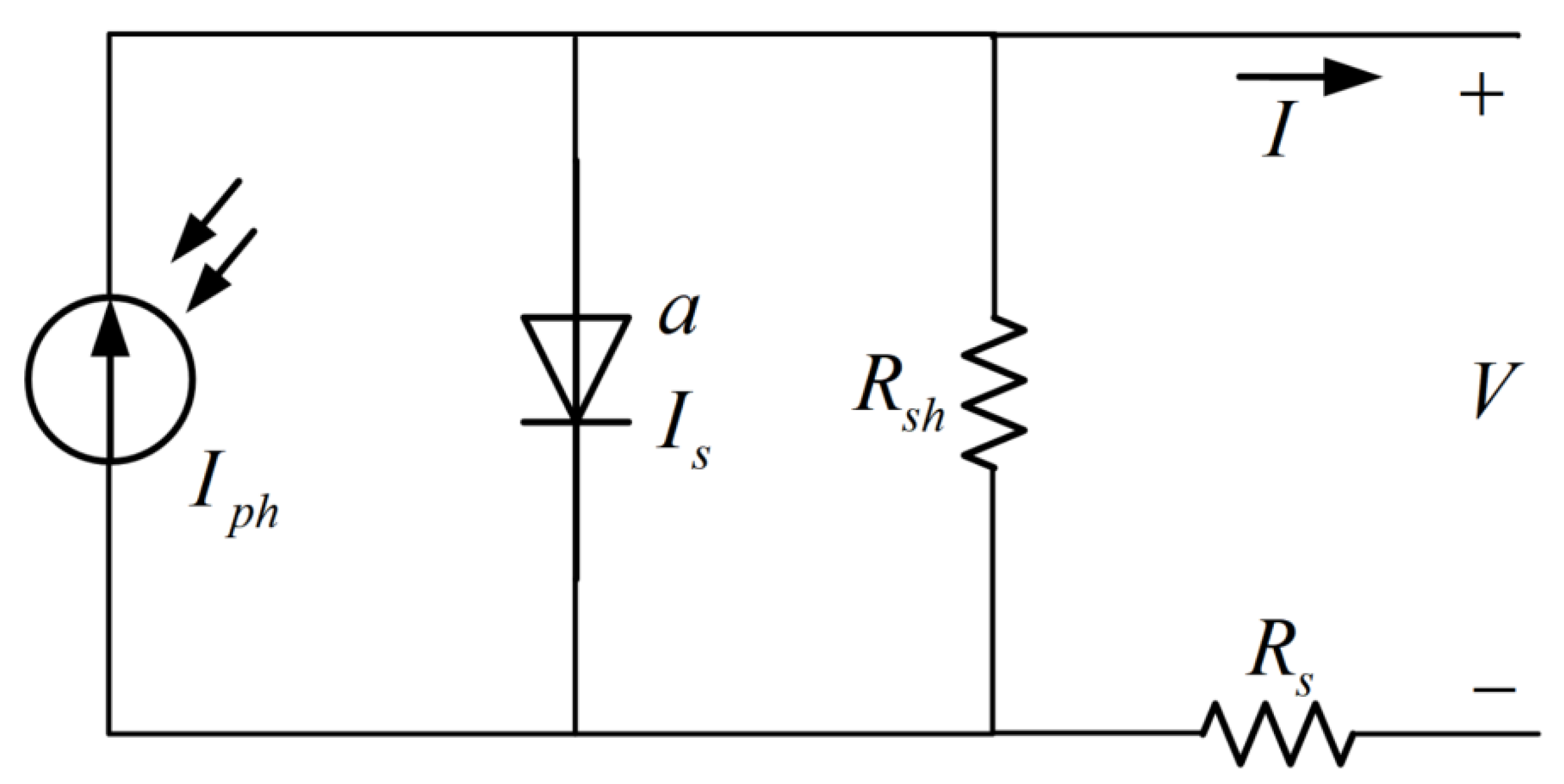
A single-diode lumped-parameter equivalent circuit is shown in Figure 1 [20]. Here, there are five parameters that need to be defined to simulate the I-V characteristics of solar cells.

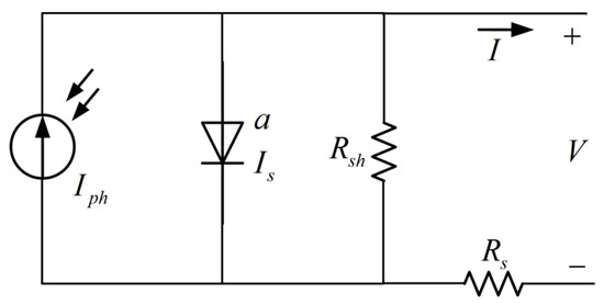
Figure 1. Single-diode lumped-parameter equivalent circuit model.

According to Kirchhoff’s current law and Schottky’s diode ideal current equation, the relationship between the terminal current and voltage (I-V) can be written by [20]:

$$I=I_{ph}-I_s(e^{\frac{V+I{R}_s}{a}}-1)-\frac{V+I{R}_s}{R_{sh}}$$

(1)

Equation (1) is a transcendental function, where I is the output current and V is the output voltage. I_ph, I_s, a, R_s and R_sh are five parameters that need to be extracted, where I_ph is the photovoltaic current source, I_s is the reverse saturation current of the diode, a is the ideality factor of the diode, R_s is the series resistance, and R_sh is the parallel resistance.

In order to calculate the {I_ph, I_s, a, R_s, R_sh} values, we require at least five equations. On the one hand, we can obtain three equations at three special points in the I-V characteristic, including the open-circuit voltage point, short-circuit current point and the maximum power point. It is noted that these three points can be found out in datasheet. On the other hand, the slopes of the I-V curve at these three points can be acquired from the reconstructed experimental results or PV manufacturers’ data [21,22]. Notably, these three special points are directly substituted into (1), yielding the following nonlinear equations. At the short-circuit current point (V = 0, I = I_sc), Equation (1) becomes:

$$I_{sc}=I_{ph}-I_s(e^{\frac{I_{sc}{R}_s}{a}}-1)-\frac{I_{sc}{R}_s}{R_{sh}}$$

(2)

At the open-circuit voltage point (V = V_oc, I = 0), Equation (1) is reformulated as:

$$0=I_{ph}-I_s(e^{\frac{V_{oc}}{a}}-1)-\frac{V_{oc}}{R_{sh}}$$

(3)

At the maximum power point (V = V_m, I = I_m), Equation (1) is rewritten as:

$$I_m=I_{ph}-I_s\left(e^{\frac{V_m+I_m{R}_s}{a}}-1\right)-\frac{V_m+I_m{R}_s}{R_{sh}}.$$

(4)

Equations (2)–(4) are three independent equations with five unknown variables: I_ph, I_s, a, R_s and R_sh. Additionally, another three equations could be established according to the slopes of I-V characteristics at the three simultaneous special points. By differentiating V with respect to I in Equation (1), we obtain:

$$\frac{dV}{dI}=-\frac{1}{\frac{1}{R_{sh}}+\frac{I_s}{a}{e}^{\frac{V+I{R}_s}{a}}}-R_s.$$

(5)

The slopes of the I-V curve at the short-circuit current and the open-circuit voltage points can be expressed by R_sc and R_oc, respectively:

$$R_{sc}=-\left(\frac{dV}{dI}\right){|}_{I=I_{sc}}$$

(6)

$$R_{oc}=-\left(\frac{dV}{dI}\right){|}_{V=V_{oc}}.$$

(7)

By substituting Equations (6) and (7) into (5), the following equations are acquired as:

$$\frac{1}{R_{sh}}-\frac{1}{R_{sc}-R_s}+\frac{I_s}{a}{e}^{\frac{I_{sc}{R}_s}{a}}=0$$

(8)

$$\frac{1}{R_{oc}-R_s}-\frac{1}{R_{sh}}-\frac{I_s}{a}{e}^{\frac{V_{oc}}{a}}=0.$$

(9)

In addition, the derivative of power to voltage is zero at the maximum power point, so the slope of this point can be obtained as:

$$\frac{dP}{dV}{|}_{P=P_m}=V_m\frac{dI}{dV}+I_m\frac{dV}{dV}=0$$

(10)

$$\frac{dI}{dV}{|}_{P=P_m}=-\frac{I_m}{V_m}.$$

(11)

Then, by substituting Equation (11) into (5), we obtain:

$$\frac{I_m}{V_m}=\frac{I_s}{a}\left(1-R_s\frac{I_m}{V_m}\right)e^{\frac{V_m+I_m{R}_s}{a}}+\frac{1}{R_{sh}}\left(1-R_s\frac{I_m}{V_m}\right).$$

(12)

Six equations—(2), (3), (4), (8), (9), and (12)—form a transcendental equation set, where five model parameters can be solved analytically.

The results are as follows:

$$R_s=R_{sc}\frac{A}{A-B}-\frac{V_m}{I_m}\frac{B}{A-B}$$

(13)

where:

$$A=(I_{sc}-\frac{V_{oc}}{R_{sc}})(\frac{V_m}{I_m}-R_{oc})$$

and:

$$B=\left(I_m-\frac{V_{oc}-V_m}{R_{sc}}\right)\left(R_{sc}-R_{oc}\right).$$

$$R_{sh}=\frac{\left(I_{sc}{R}_s-V_{oc}\right)C-\left[I_m{R}_s-\left(V_{oc}-V_m\right)\right]D}{I_{m}D-I_{sc}C}$$

(14)

where:

$$C=(\frac{V_m}{I_m}-R_{oc})(R_{sc}-R_s)$$

and:

$$D=\left(\frac{V_m}{I_m}-R_s\right)\left(R_{sc}-R_{oc}\right).$$

$$I_{ph}=I_{sc}\left(1+\frac{R_s}{R_{sh}}\right).$$

(15)

$$a=\frac{\left[I_{sc}(1+\frac{R_s}{R_{sh}})-\frac{V_{oc}}{R_{sh}}\right]\left(R_{oc}-R_s\right)\left(R_{sc}-R_s\right)}{\left(R_{sc}-R_{oc}\right)}.$$

(16)

$$I_s=\frac{I_{sc}(1+\frac{R_s}{R_{sh}})-\frac{V_{oc}}{R_{sh}}}{e^{\frac{V_{oc}}{a}}-e^{\frac{I_{sc}{R}_s}{a}}}.$$

(17)

3. Verification and Discussion

In this section, numerical simulations and reconstructed experimental data are necessary to validate the parameter estimation algorithm of the solar cell model. In order to verify the accuracy and efficiency of our parameter estimation method, the original I-V curve based on numerical simulations with the settled parameters is contrasted, with the curves simulated by using the estimated parameters. Furthermore, the experimental data from solar cells of the I-V curves are used to validate the universality of our parameter extraction algorithm.

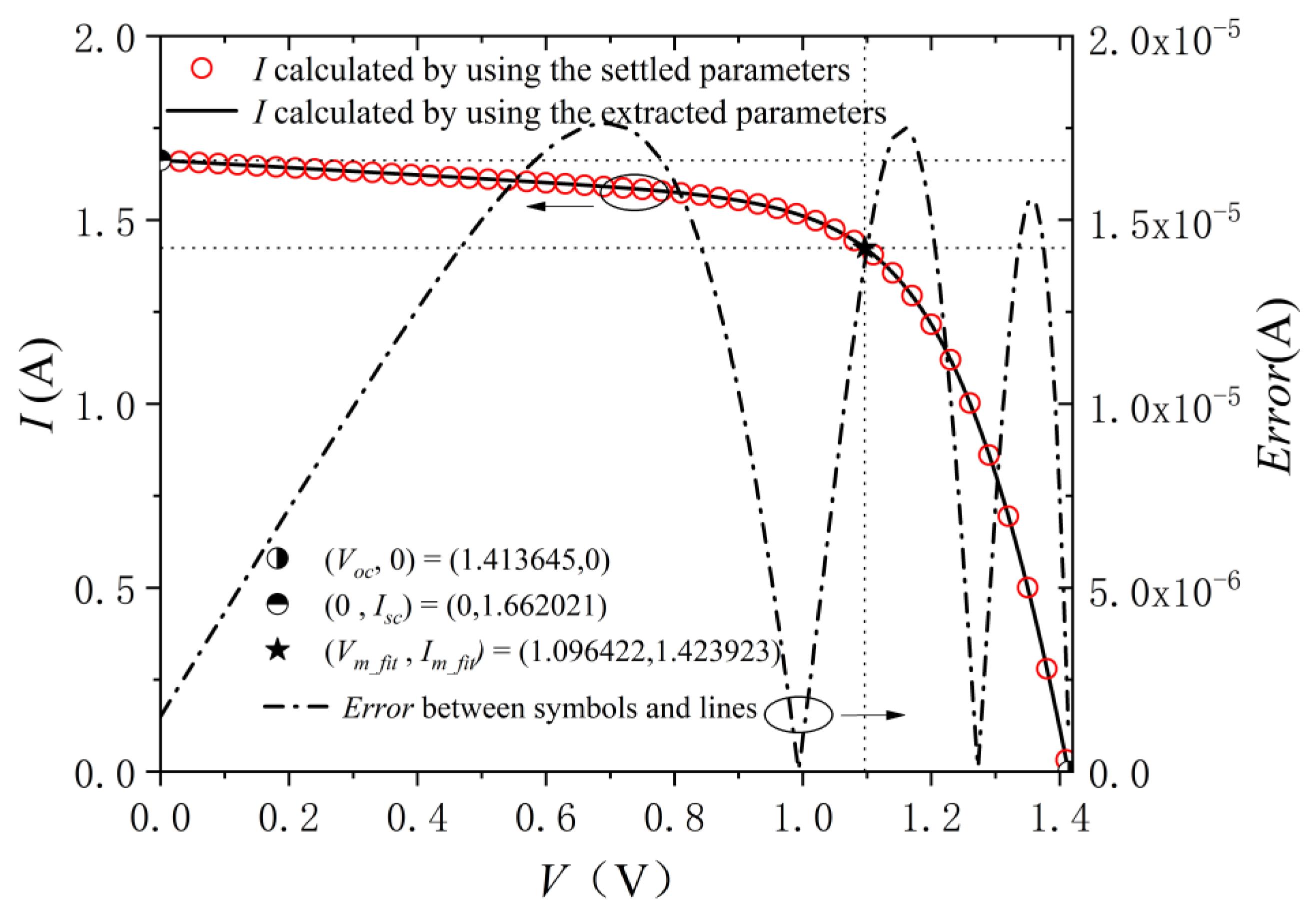
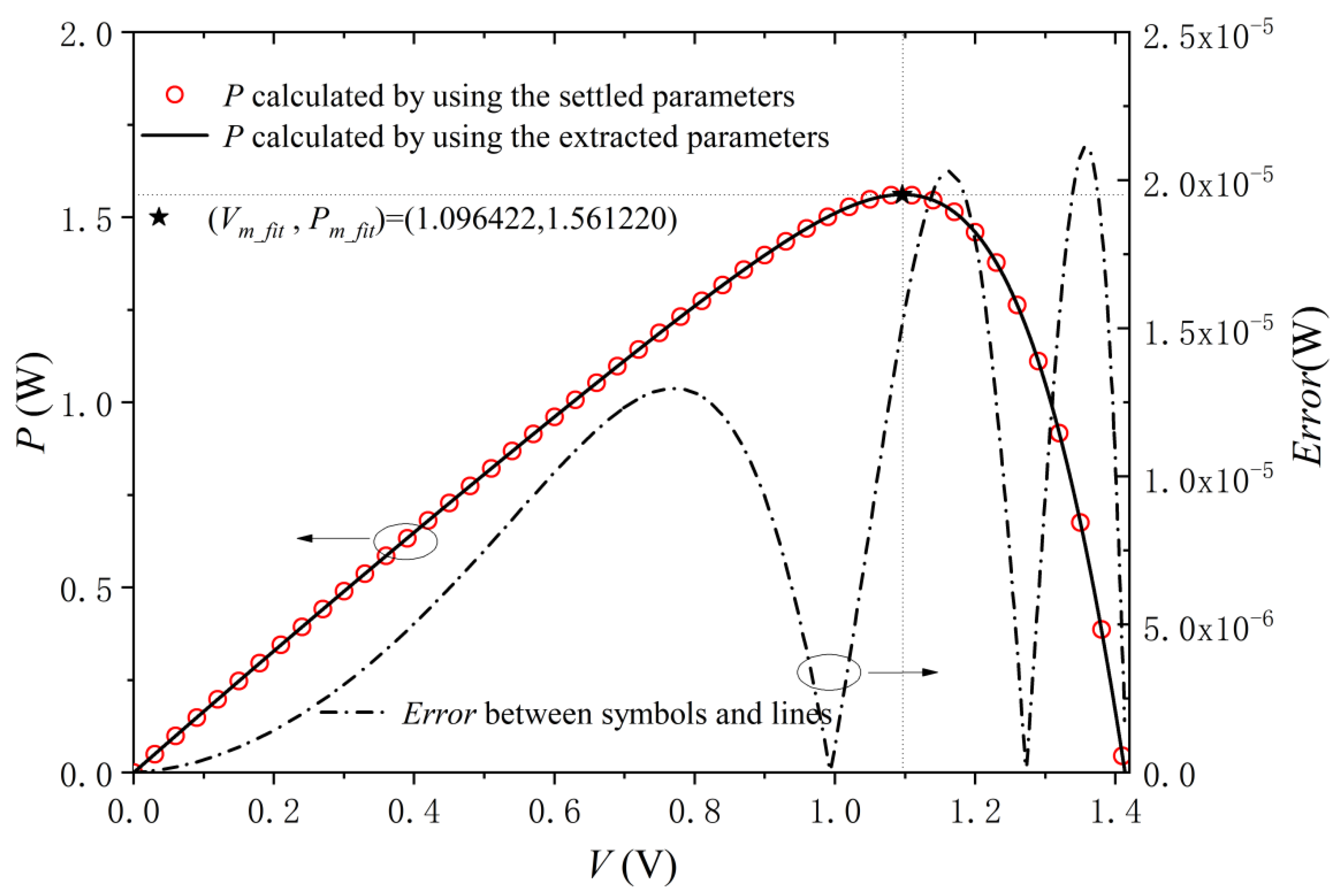
The I- and P-V characteristics, based on the numerical simulations with the settled parameters, are shown in Figure 2 and Figure 3, respectively. By using our above analytical algorithm of parameter extraction, we can define all five model parameters listed in Table 1 and reproduce I- and P-V curves with the extracted parameters in Figure 2 and Figure 3. Here, we notice that I- and P-V curves have a good agreement by using the estimated and settled parameters. The absolute errors of the two curves in Figure 2 are within 2 × 10⁻⁵ A, and those in Figure 3 are less than 2.5 × 10⁻⁵ W. It is observed that the maximum errors of P-V characteristics is located near the open circuit voltage point (V_oc, 0). The reason for this is that the coefficient $\frac{R_s}{R_{sh}}$ of I_m is ignored, and the coefficient $\frac{1}{R_{sh}}$ of V_m and V_oc is replaced by $\frac{1}{R_{sc}}$, in the processs of equality simplification. In Table 1, we can observe that the minimum relative error between the settled and extracted parameters is below 5‰. In Table 2, it also can be seen that the relevant factors obtained from the original curve and calculated from I-V curve with the extracted parameters have a high consistency.

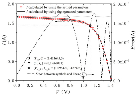
Figure 2. Comparison of calculated I-V characteristics with the settled and estimated parameters shown in Table 1, and the absolute errors between symbols and lines.

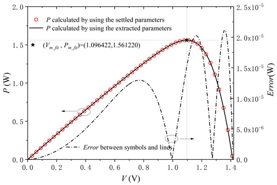
Figure 3. Comparison of calculated P-V characteristics with the settled and estimated parameters shown in Table 1, and the absolute errors between symbols and lines.

Table 1. Parameters estimation values of our algorithm.

Symbols	Settled Model Parameters	Extracted Model Parameters
Iph (A)	1.670000	1.670005
Is (μA)	1.250000	1.245185
a	0.100854	0.100826
Rsh (Ω)	10.00000	9.997104
Rs (Ω)	0.048000	0.048024

Table 2. Relevant factors in I- and P-V curves calculated by using the settled and extracted parameters.

Relevant Factors	Settled Model Parameters	Extracted Model Parameters
Isc (A)	1.662020	1.662019
Voc (V)	1.413645	1.413645
P(W) = Isc × Voc	2.349507	2.349504
Im (A)	1.423923	1.423924
Vm (V)	1.096422	1.096432
Pm(W) = Im × Vm	1.561220	1.561236
FF = Pm/(Voc × Isc)	66.4489%	66.4496%
Rsc (Ω)	10.04513	10.04234
Roc (Ω)	0.113551	0.113605

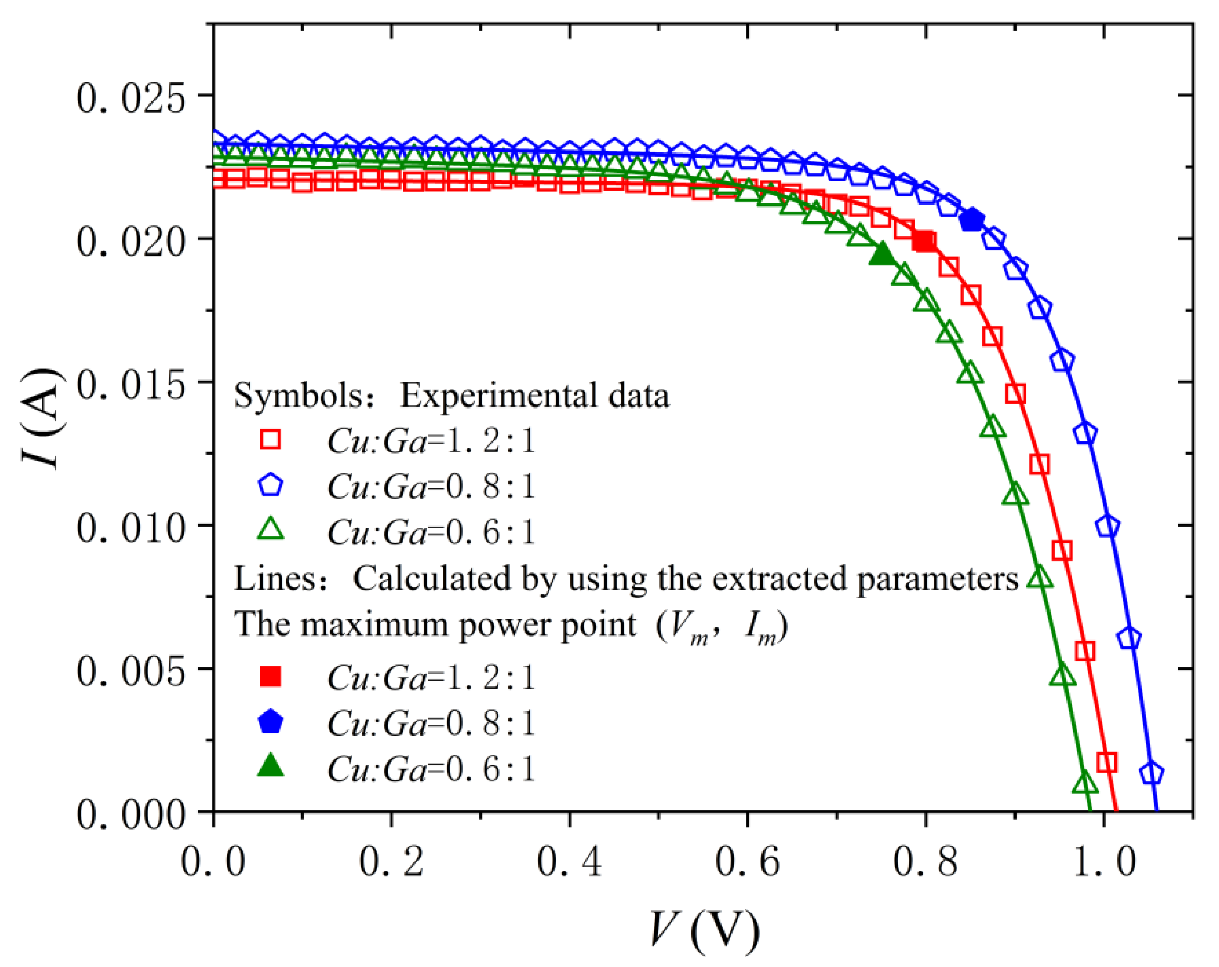
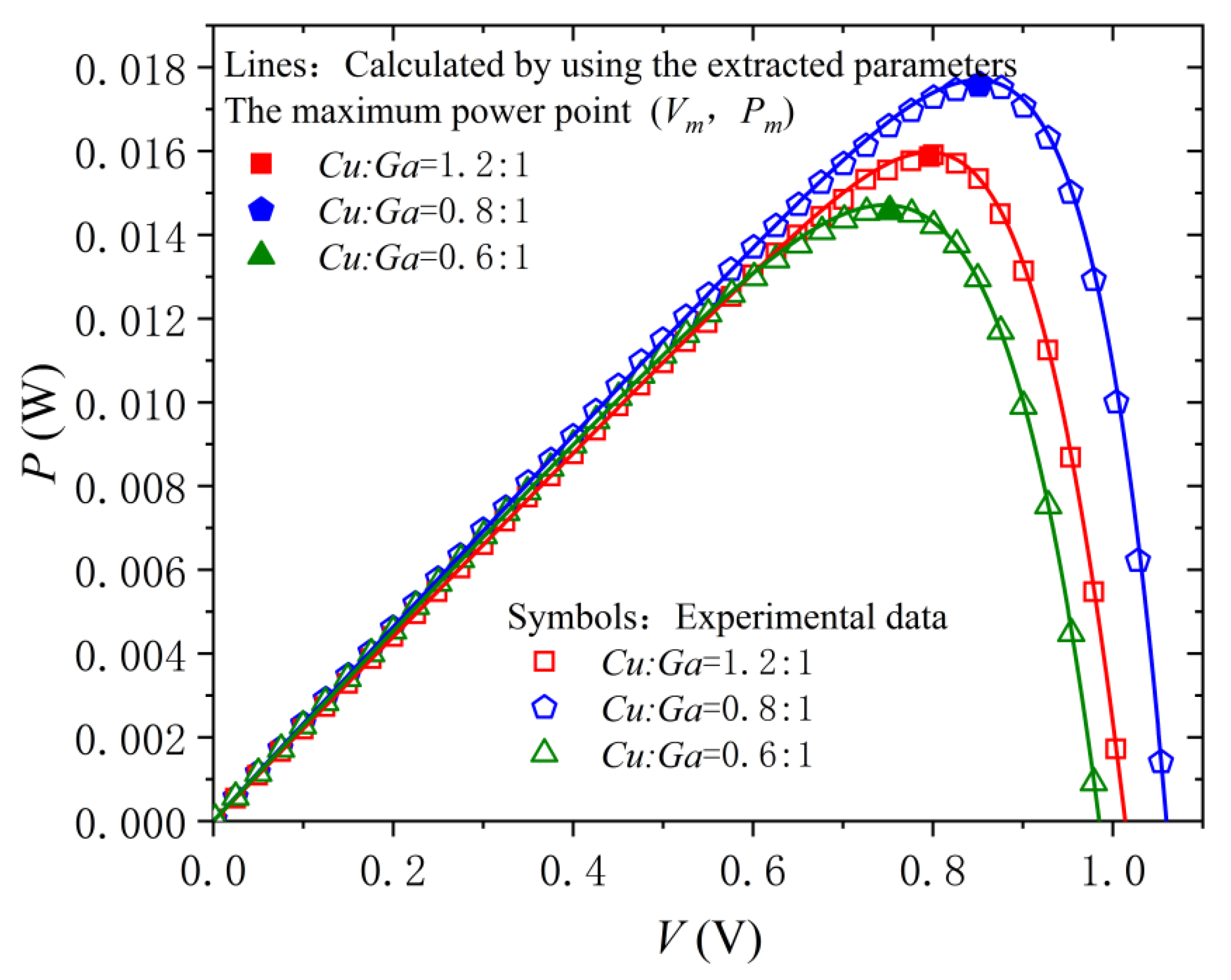
Figure 4 and Figure 5 show the reconstructed experimental data [20] and simulation results by using the parameters estimated through our method described above. Figure 6 illustrates the absolute errors in Figure 4. The estimated parameter values are summarized in Table 3, and their relevant factors, calculated from our parameter estimation method, are shown in Table 4, where these factors of the curve obtained by polynomial fitting and the curve solved by the extracted parameter values are also compared.

Figure 4. I-V characteristics measured and calculated, respectively.

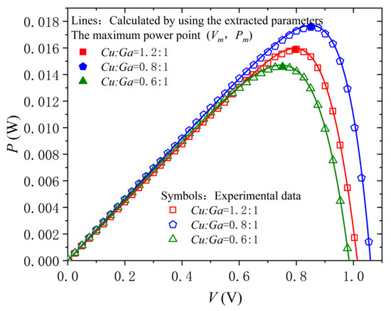
Figure 5. P-V characteristics measured and calculated, respectively.

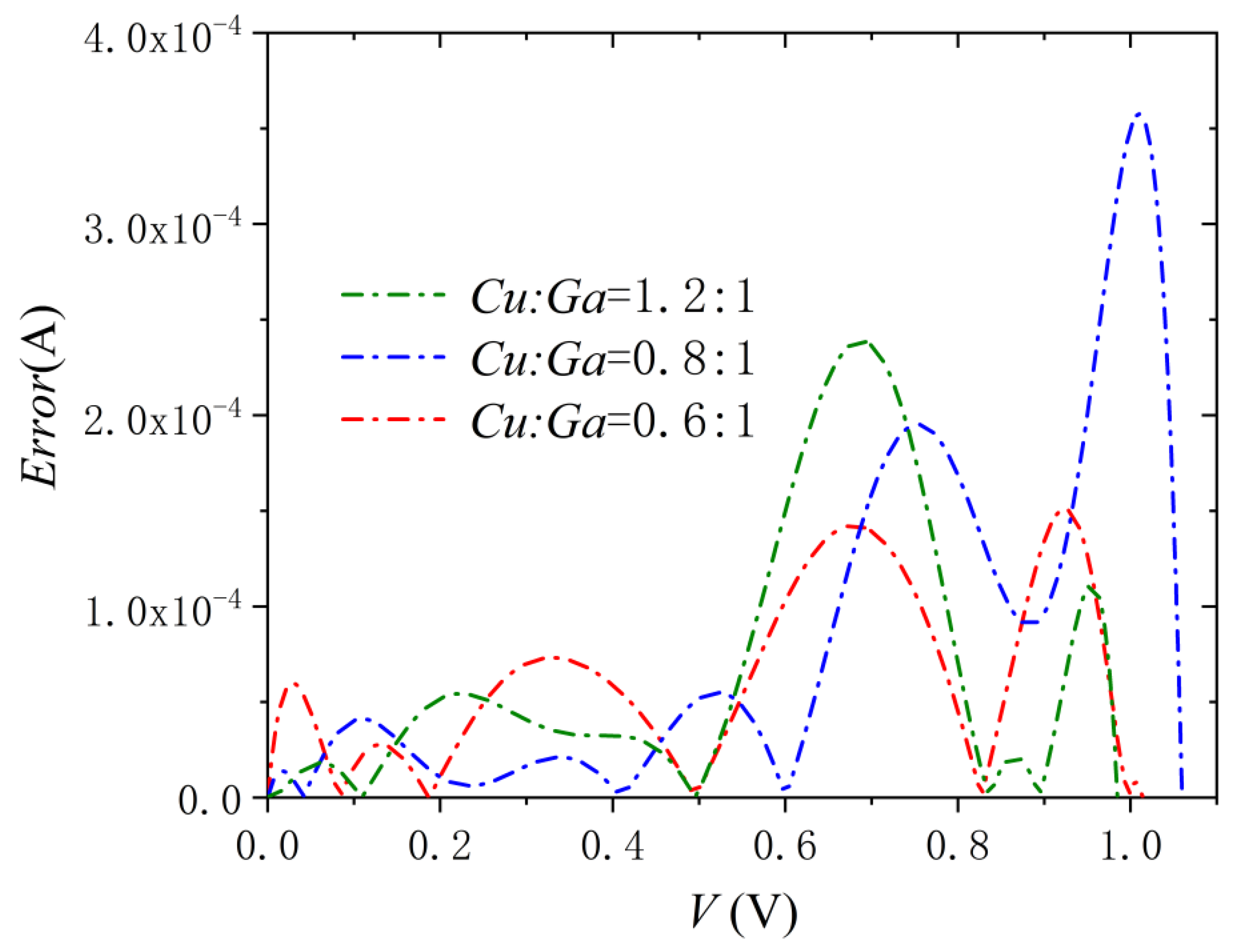
Figure 6. Absolute errors of I-V characteristics between symbols and lines in Figure 4.

Table 3. Parameter estimation values for I- and P-V characteristics in Figure 4 and Figure 5.

Cu:Ga	1.2:1	0.8:1	0.6:1
Iph (A)	0.0220853	0.0233143	0.0228886
Is (A)	4.3673630 × 10−9	2.7389066 × 10−8	7.2781006 × 10−7
Rs (Ω)	2.6339570	0.8082216	1.6242257
Rsh (Ω)	3352.4723	1437.2007	1211.0273
a	0.0657331	0.0777924	0.0954416

Table 4. Relevant factors acquired by extracted parameters calculation and experimental curve fitting in I- and P-V curves.

Cu:Ga	1.2:1		0.8:1		0.6:1
Parameters	Symbol	Line	Symbol	Line	Symbol	Line
Isc (A)	0.022068	0.022068	0.023301	0.023301	0.022856	0.022855
Voc (V)	1.013767	1.013767	1.059711	1.059710	0.984946	0.984944
P(W) = Isc × Voc	0.022372	0.022372	0.024692	0.024692	0.022512	0.022511
Im (A)	0.019924	0.020075	0.020654	0.020821	0.019381	0.019694
Vm (V)	0.796342	0.795425	0.852356	0.849933	0.752065	0.746969
Rsc (Ω)	3355.106	3354.243	1438.009	1440.564	1012.652	1012.078
Roc (Ω)	5.938071	5.913439	4.589079	4.585644	6.271030	6.214534
Pm(W) = Im × Vm	0.015866	0.015968	0.017604	0.017697	0.014576	0.014711
FF = Pm/(Voc × Isc)	70.9209%	71.3756%	71.2947%	71.6678%	64.7478%	65.3480%

In reference [23], prepared CuGaS₂ quantum dots (CGS QDs) were used as hole-transport materials (HTM) for perovskite solar cells (PSCs). Due to the inevitable flaws of inorganic nanoparticles, which could have an influence on the properties of PSCs, this study accurately controlled the Cu content and systematically studied its impact on the photovoltaic performance of solar cells.

First, good agreements are observed in Figure 4 and Figure 5. In addition, the absolute error of the two curves in Figure 6 is within 4 × 10⁻⁴ A. The error curve varies in wave shape. The voltage relationship of the error peak value is consistent with the relationship of the maximum power voltage value. The relationship of the maximum power voltage value from small to large is 0.6:1,1.2:1,0.8:1 (Cu:Ga, molar ratio) in order, and the voltage relationship corresponding to the error peak value is also 0.6:1,1.2:1,0.8:1 (Cu:Ga, molar ratio).

Second, the impact of parameters on the curve can also be shown from the curves. The parameter I_ph is very approaching to the short-circuit current I_sc, which represents the intercept with the ordinate axis of the I-V curve. It can be seen that the order of intercept from large to small is 0.8:1,0.6:1,1.2:1 (Cu:Ga, molar ratio) in Figure 4, and the parameter value I_ph also conforms to the law of the image. The parallel resistance value R_sh and the series resistance value R_s are consistent with the slope of the curve at 0 V < V < V_m and V_m < V < V_oc. On the one hand, it can be observed that, when 0 V < V < V_m, as the ratio of Cu to Ga, decreases, the slope also decreases, and the value of R_sh also decreases, as shown in Table 3. On the other hand, for series resistance R_s, when V_m < V < V_oc the order of slope from large to small is 1.2:1,0.6:1,0.8:1(Cu:Ga, molar ratio). From Table 3, it can be seen that the relationship of R_s is 1.2:1 > 0.6:1 > 0.8:1(Cu:Ga, molar ratio) similarly. Apart from this, both I_s and a increase as the Cu:Ga ratio decreases.

Third, the relevant factors (including I_sc, V_oc, P_m, R_oc, R_sc and FF) of I- and P-V curves acquired by the calculation of extracted parameters are compared with those acquired by experimental curve fitting. It is worth noting that the symbols’ parameters have a good correlation with the lines’ parameters, and their maximum relative error is below 1%. The filling factor FF of the PSCs based on CuCaS₂ increases from approximately 70.9209% to 71.2947%, while the Cu content is reduced from 1.2:1 to 0.8:1 (Cu:Ga, molar ratio). Nevertheless, as the Cu content further decreases to 0.6:1, the property of PSCs becomes worse.

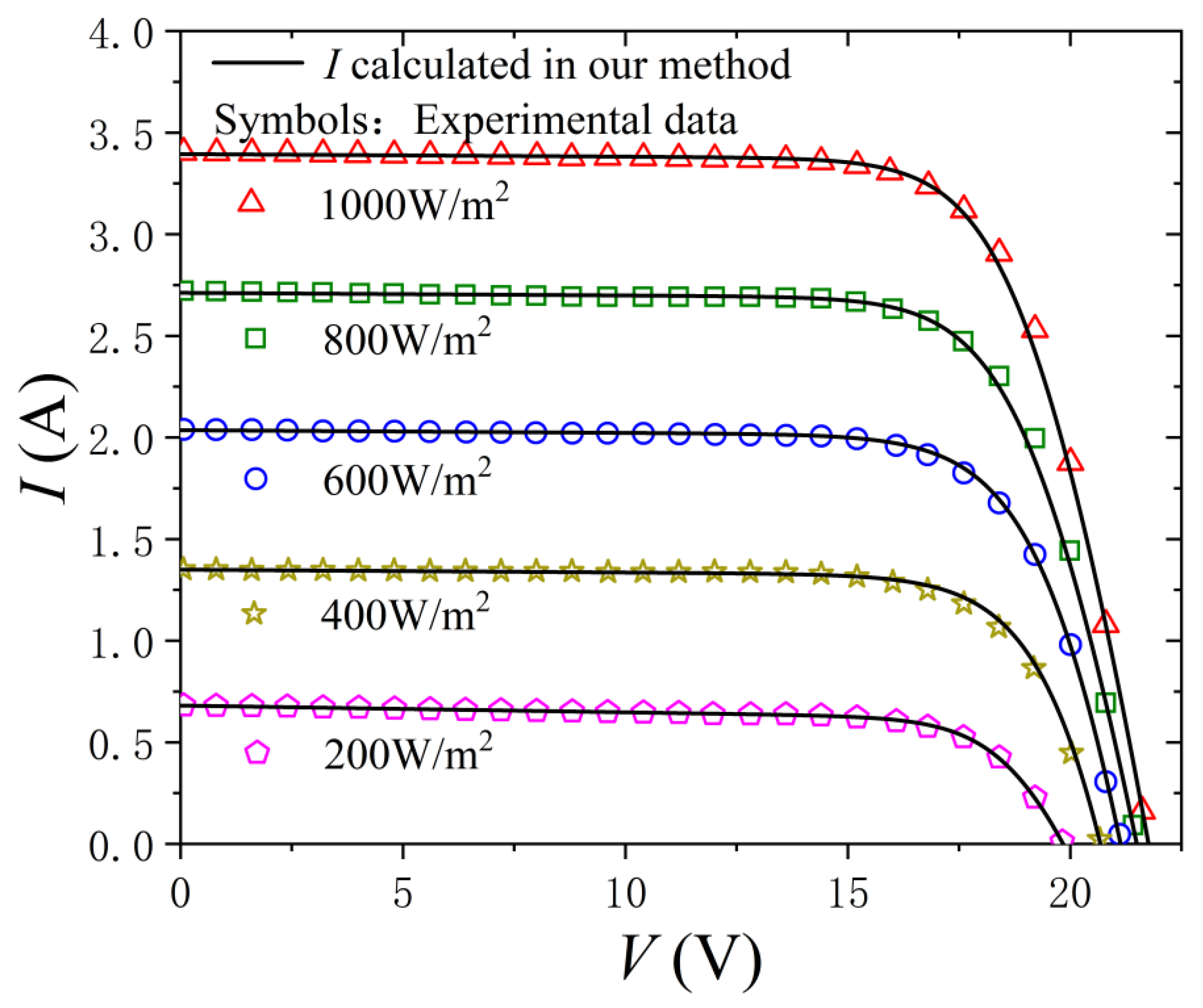
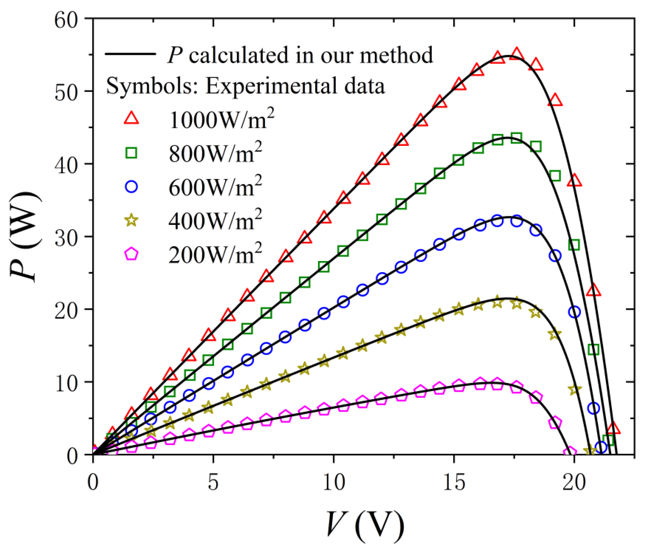
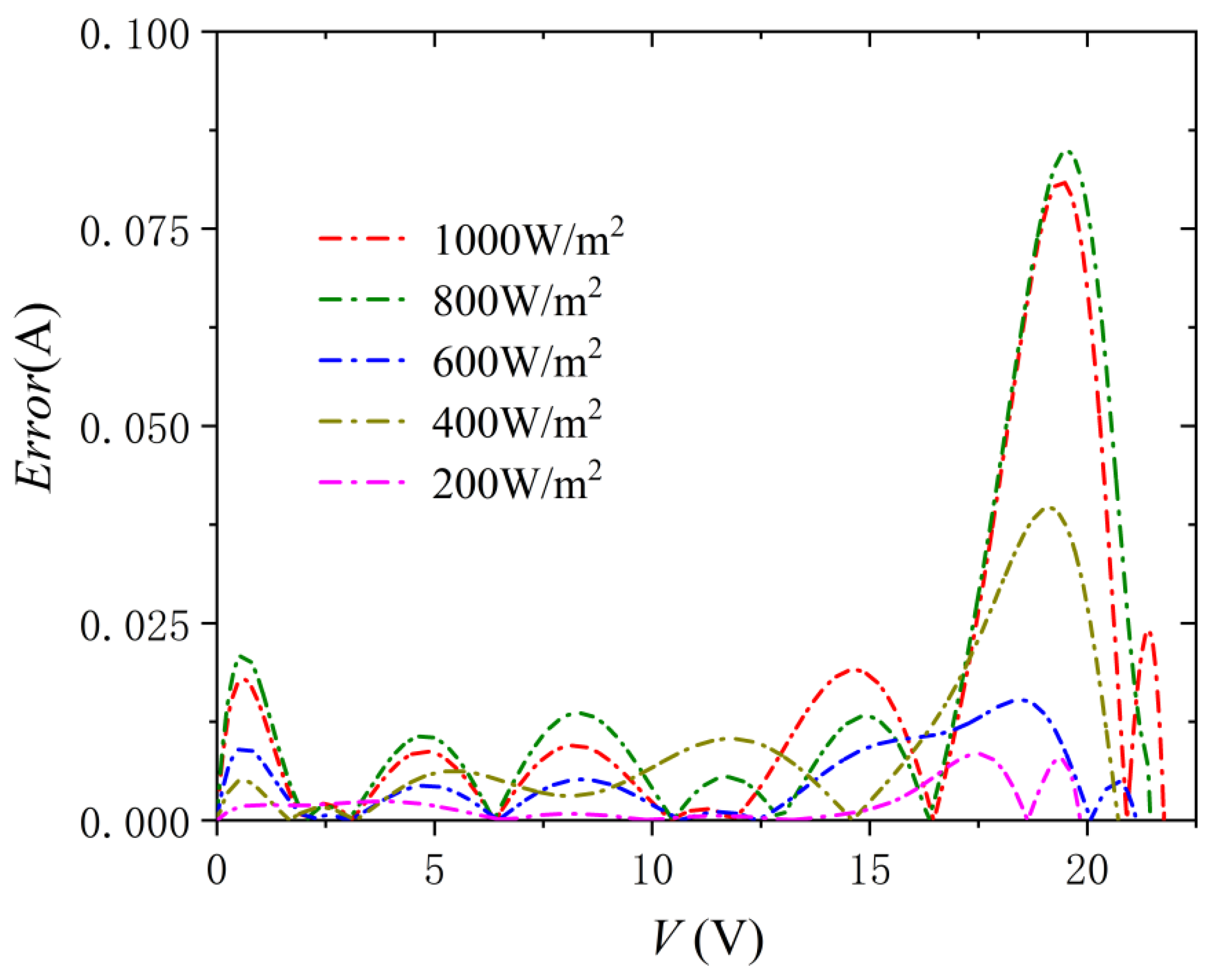
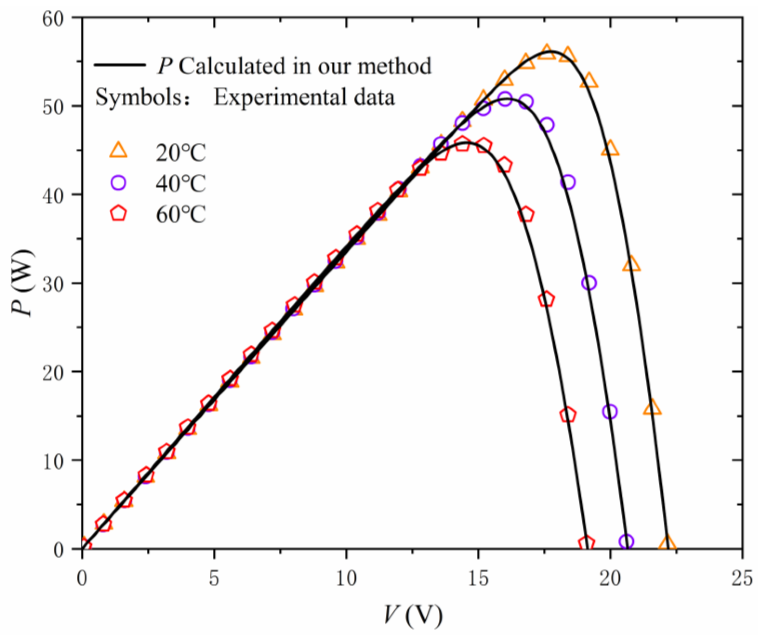
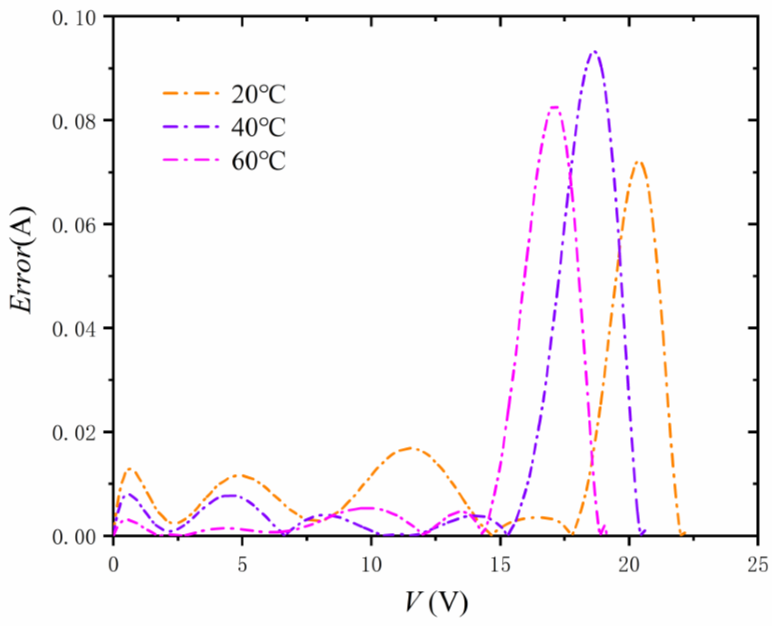
Figure 7, Figure 8, Figure 9, Figure 10, Figure 11 and Figure 12 illustrate the modeled I- and P-V characteristics regarding the experimental data for the SM55 PV model [24] under different irradiance and temperature levels. The results show that the simulation results of the proposed model match closely with the experimental measurements. The absolute errors between modeled and measured results are also shown. The variable is irradiance, which ranged from 200 W/m² up to 1000 W/m² at a certain temperature of 25 °C, as shown in Figure 7 and Figure 8. When the irradiance increases, the short-circuit current I_sc will increase, but the open-circuit voltage V_oc has little change. Furthermore, the accuracy of the proposed algorithm was experimentally evaluated. Figure 9 shows the absolute errors in Figure 7. The absolute error of the two curves was below 0.1 A, and the shape of the error change is the waveform. Under fixed-temperature conditions, the voltage values of the maximum power point are almost the same, as well as the positions of the maximum error. Similarly, the variable that is controlled in Figure 10 and Figure 11 is temperature, increasing from 20 °C to 60 °C, and the irradiance is kept at a constant value of 1000 W/m². The increasing temperature reduces V_oc, and I_sc does not change much. Figure 12 shows the absolute errors in Figure 10. The absolute error of the two curves is less than 0.1 A, and the error varies in different waves. Under different temperature conditions, the voltage values of the maximum power point and the voltage values of the maximum error decrease with the increase in temperature. The five parameters are also extracted by using the equations in the previous section, given in Table 5 and Table 6. Therefore, the proposed algorithm has a high accuracy and can simulate the I- and P-V curves for a PV module under any operating conditions. Under dim indoor light conditions, R_S and R_sh play quite different roles from those under outdoor sunlight. Under the outdoor condition, the photovoltaic performance is likely to be governed by R_S [25,26].

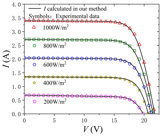
Figure 7. I-V characteristics measured and calculated, respectively, for the thin-film SM55 PV panel in different irradiance conditions.

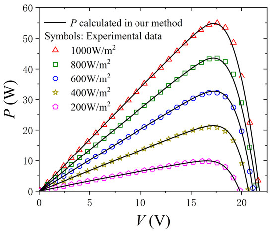
Figure 8. P-V characteristics measured and calculated, respectively, for the thin-film SM55 PV panel in different irradiance conditions.

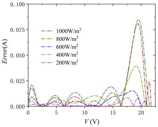
Figure 9. Absolute errors of I-V characteristics between symbols and lines in Figure 7.

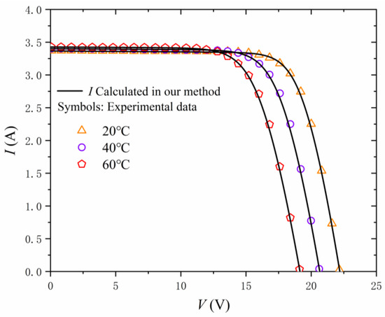
Figure 10. I-V characteristics measured and calculated, respectively, for the thin-film SM55 PV panel in different temperature conditions.

Figure 11. P-V characteristics measured and calculated, respectively. for the thin-film SM55 PV panel in different temperature conditions.

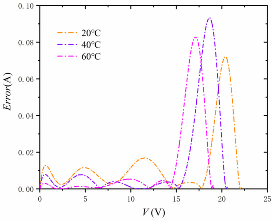
Figure 12. Absolute errors of I-V characteristics between symbols and lines in Figure 10.

Table 5. Parameter estimation values for I- and P-V characteristics in Figure 7 and Figure 8.

Irradiance (W/m2)	1000	800	600	400	200
Iph (A)	3.3962417	2.7131558	2.0363498	1.3493865	0.6827725
Is (A)	7.308938 × 10−10	1.403863 × 10−9	1.092685 × 10−8	8.576250 × 10−9	8.328075 × 10−11
Rs (Ω)	0.5430073	0.5676721	0.4013254	0.3015109	1.0673264
Rsh (Ω)	788.55654	776.54018	765.691502	728.019704	300.01679
a	0.9779623	1.0057922	1.1105125	1.0968676	0.8729821

Table 6. Parameter estimation values for I- and P-V characteristics in Figure 10 and Figure 11.

Parameters	20 °C	40 °C	60 °C
Iph (A)	3.3683097	3.4030083	3.4286977
Is (A)	9.2486844 × 10−11	5.9109404 × 10−9	5.3839465 × 10−8
Rs (Ω)	0.5621175	0.5656343	0.5869989
Rsh (Ω)	732.52200	788.74959	864.79641
a	0.9129523	1.0244086	1.0653797

4. Conclusions

In this paper, an analytical model parameter extraction algorithm of a lumped-parameter equivalent circuit of solar cells was proposed. The proposed parameter-extraction algorithm was also able to be carried out in simulation platforms for different kinds of solar cells under the different conditions of materials, processes, and environments. As a result, it was proven that the proposed method was good algorithm for simulating the I- and P-V curves of perovskite solar cells and PV panels, and a good tool for systematically investigating the influence of material composition on the optical–electrical characteristics of the solar cells. In addition, it provides a feasible algorithm for studying the comprehensive performance of perovskite solar cells and PV panels.

References

- Wang, Y.B.; Liu, X.; Zhou, Z.M.; Ru, P.B.; Chen, H.; Yang, X.D.; Han, L.Y. Reliable measurement of perovskite solar cells. Adv. Mater. 2019, 31, 1803231. [Google Scholar] [CrossRef]
- Boutana, N.; Mellit, A.; Haddad, S.; Rabhi, A.; Pavan, A.M. An explicit IV model for photovoltaic module technologies. Energy Convers. Manag. 2017, 138, 400–412. [Google Scholar] [CrossRef]
- Senturk, A.; Eke, R. A new method to simulate photovoltaic performance of crystalline silicon photovoltaic modules based on datasheet values. Renew. Energy 2016, 103, 58–69. [Google Scholar] [CrossRef]
- Fallahazad, P.; Naderi, N.; Eshraghi, M.J. Improved photovoltaic performance of graphene-based solar cells on textured silicon substrate. J. Alloys Compd. 2020, 834, 155123. [Google Scholar] [CrossRef]
- Batzelis, I.E. Simple PV performance equations theoretically well founded on the single-diode model. IEEE J. Photovolt. 2017, 7, 1400–1409. [Google Scholar] [CrossRef]
- Brano, V.L.; Orioli, A.; Ciulla, G.; Gangi, A.D. An improved five-parameter model for photovoltaic modules. Sol. Energy Mater. Sol. Cells 2010, 94, 1358–1370. [Google Scholar] [CrossRef]
- Phang, J.C.H.; Chan, D.S.H.; Phillips, J.R. Accurate analytical method for the extraction of solar cell model parameters. Electron. Lett. 1984, 20, 406–408. [Google Scholar] [CrossRef]
- Batzelis, E. Non-iterative methods for the extraction of the single-diode model parameters of photovoltaic modules: A review and comparative assessment. Energies 2019, 12, 358. [Google Scholar] [CrossRef] [Green Version]
- Ortiz-Conde, A.; García-Sánchez, F.J.; Muci, J.; Sucre-González, A. A review of diode and solar cell equivalent circuit model lumped parameter extraction procedures. FU Electron. Energetics 2014, 27, 57–102. [Google Scholar] [CrossRef]
- Cubas, J.; Pindado, S.; Victoria, M. On the analytical approach for modeling photovoltaic systems behavior. J. Power Sources 2013, 247, 467–474. [Google Scholar] [CrossRef] [Green Version]
- Khan, F.; Baek, S.; Park, Y.; Kim, J.H. Extraction of diode parameters of silicon solar cells under high illumination conditions. Energy Convers. Manag. 2013, 76, 421–429. [Google Scholar] [CrossRef]
- Yu, F.; Huang, G.; Xu, C. An explicit method to extract fitting parameters in lumped-parameter equivalent circuit model of industrial solar cells. Renew. Energy 2019, 146, 2188–2198. [Google Scholar] [CrossRef]
- Wei, T.; Yu, F.; Huang, G.; Xu, C. A particle-swarm-optimization-based parameter extraction routine for three-diode lumped parameter model of organic solar cells. IEEE Electron. Device Lett. 2019, 40, 1511–1514. [Google Scholar] [CrossRef]
- Toledo, F.J.; Blanes, J.M.; Galiano, V. Two-step linear least-squares method for photovoltaic single-diode model parameters extraction. IEEE Trans. Ind. Electron. 2018, 65, 6301–6308. [Google Scholar] [CrossRef]
- García-Sánchez, F.J.; Ortiz-Conde, A.; Mercato, G.D.; Liou, J.J.; Rechi, L. Eliminating parasitic resistances in parameter extraction of semiconductor device models. In Proceedings of the First International Caracas Conference on Devices, Circuits and Systems, Caracas, Venezuela, 12–14 December 1995; pp. 298–302. [Google Scholar]
- Ortiz-Conde, A.; Sánchez, F.J.G. Extraction of non-ideal junction model parameters from the explicit analytic solutions of its I–V characteristics. Solid State Electron. 2004, 49, 465–472. [Google Scholar] [CrossRef]
- Nacar, M.; Özer, E.; Yılmaz, A.E. A six parameter single diode model for photovoltaic modules. J. Sol. Energy Eng. 2021, 143, 112. [Google Scholar] [CrossRef]
- Sharma, A.; Averbukh, M.; Jately, V.; Azzopardi, B. An effective method for parameter estimation of a solar cell. Electronics 2021, 10, 312. [Google Scholar] [CrossRef]
- Wang, J.; Yang, B.; Li, D.; Zeng, C.; Chen, Y.; Guo, Z. Photovoltaic cell parameter estimation based on improved equilibrium optimizer algorithm. Energy Convers. Manag. 2021, 236, 114051. [Google Scholar] [CrossRef]
- Shongwe, S.; Hanif, M. Comparative analysis of different single-diode PV modeling methods. IEEE J. Photovolt. 2015, 5, 938–946. [Google Scholar] [CrossRef]
- Villalva, M.G.; Gazoli, J.R.; Filho, E.R. Comprehensive approach to modeling and simulation of photovoltaic arrays. IEEE Trans. Power Electron. 2009, 24, 1198–1208. [Google Scholar] [CrossRef]
- Ishaque, K.; Salam, Z.; Taheri, H.; Syafaruddin. Modeling and simulation of photovoltaic (PV) system during partial shading based on a two-diode model. Simul. Model. Pract. Theory 2011, 19, 1613–1626. [Google Scholar] [CrossRef]
- Ma, W.; Zhang, Z.; Ma, M.; Liu, Y.; Pan, G.; Gao, H.; Mao, Y. CuGaS2 quantum dots with controlled surface defects as an hole-transport material for high-efficient and stable perovskite solar cells. Sol Energy 2020, 211, 55–61. [Google Scholar] [CrossRef]
- Shell SM55 Photovoltaic Solar Module. Available online: http://www.aeet-service.com/pdf/shell/Shell-Solar_SM55.pdf (accessed on 17 January 2017).
- Saeed, M.A.; Kim, S.H.; Kim, H.; Liang, J.; Woo, H.Y.; Kim, T.G.; Yan, H.; Shim, J.W. Indoor organic photovoltaics: Optimal cell design principles with synergistic parasitic resistance and optical modulation effect. Adv. Energy Mater. 2021, 11, 27. [Google Scholar] [CrossRef]
- Saeed, M.A.; Kang, H.C.; Yoo, K.; Asiam, F.K.; Lee, J.J.; Shim, J.W. Cosensitization of metal-based dyes for high-performance dye-sensitized photovoltaics under ambient lighting conditions. Dye. Pigment. 2021, 194, 109624. [Google Scholar] [CrossRef]
Publisher’s Note: MDPI stays neutral with regard to jurisdictional claims in published maps and institutional affiliations. |
© 2022 by the authors. Licensee MDPI, Basel, Switzerland. This article is an open access article distributed under the terms and conditions of the Creative Commons Attribution (CC BY) license (https://creativecommons.org/licenses/by/4.0/).