
Short-Term Solar Power Predicting Model Based on Multi-Step CNN Stacked LSTM Technique


Abstract
:1. Introduction
- a.
- To apply novel hybrid solar power prediction model named ‘multi-step CNN-stacked LSTM with drop-out deep learning method for improved effectiveness as compared to other traditional methods of solar irradiance forecasting.
- b.
- To forecast a highly accurate solar irradiance that would help mitigate the challenges posed by the stochastic nature of solar energy production to power grid operations.
- c.
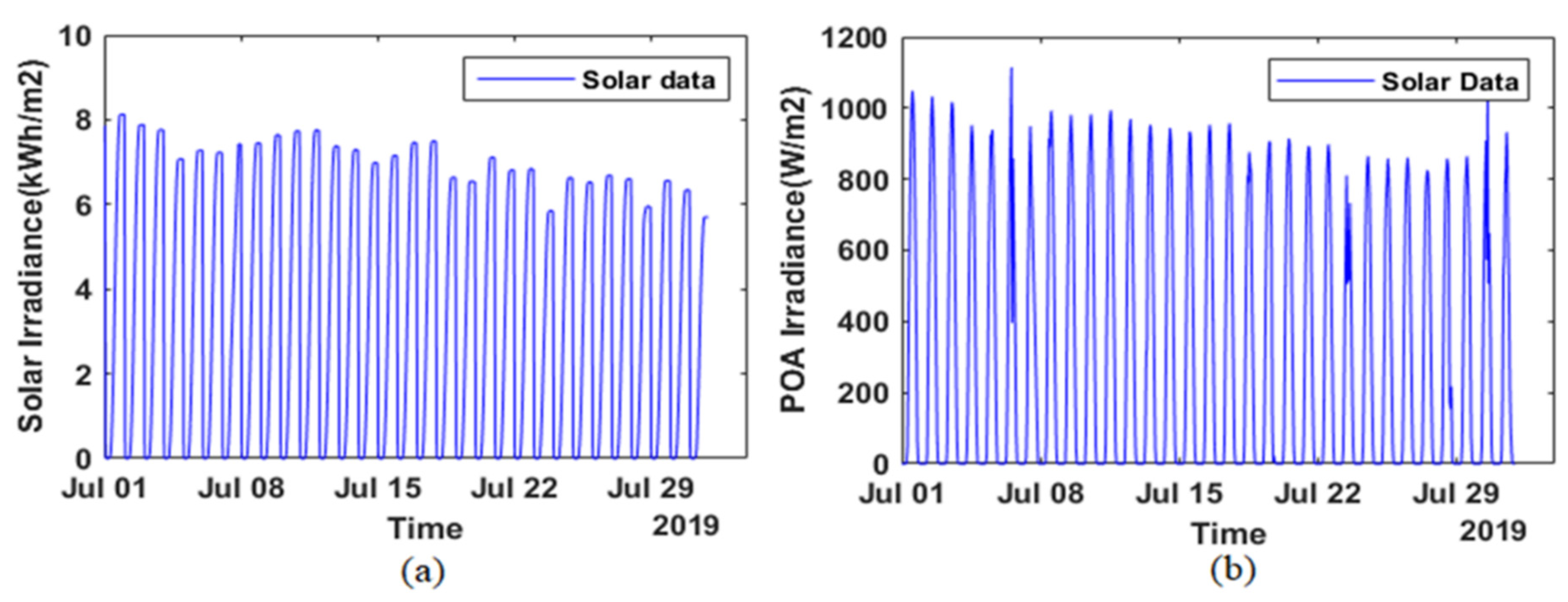
- To use real-world solar data that is taken from Sweihan Photovoltaic Independent Power Project, Abu Dhabi.
- i.
- This article provides a brief literature study on state-of-the-art solar power prediction methods, their advantage/disadvantages, and the research gap available.
- ii.
- This article presents a novel hybrid multistep CNN stacked LSTM with a drop-out model for the prediction of solar irradiance. Moreover, the POA irradiance is also forecasted as a novel application. The proposed stacked architecture and the incorporation of drop-out layers are helpful for accuracy improvement in the PV prediction model.
- iii.
- Multi-step CNN layers helped to extract features from the data and to produce sequenced data. The stacked LSTM effectively collects this data, forecasts it to improve prediction accuracy.
- iv.
- At last, the performance of the proposed solar prediction model has been validated through a detailed comparative analysis with several other contemporary ML and DL approaches such as artificial neural network and traditional LSTM model for RMSE, MAE, MAPE, R2, MSE, and NMSE. Moreover, the output of several other works that published recently are also compared with the outcome of the proposed approach.
2. Data Description and Data Preprocessing
3. Methodology
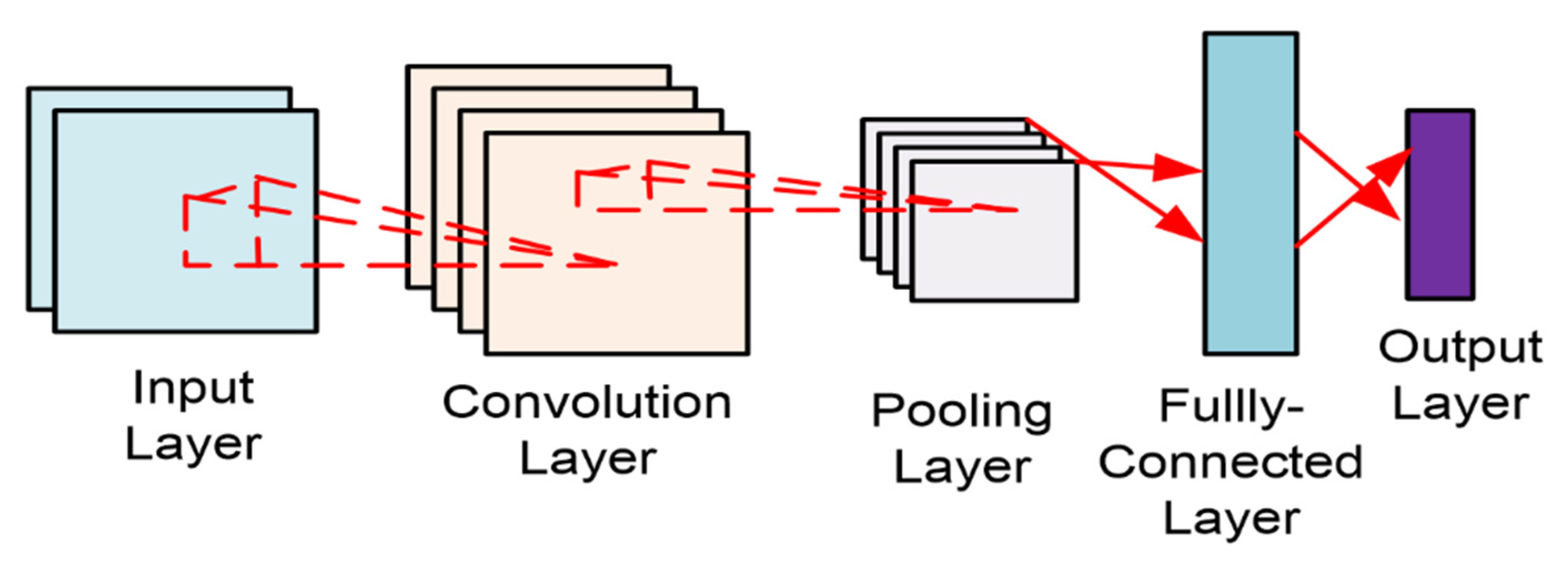
3.1. CNN
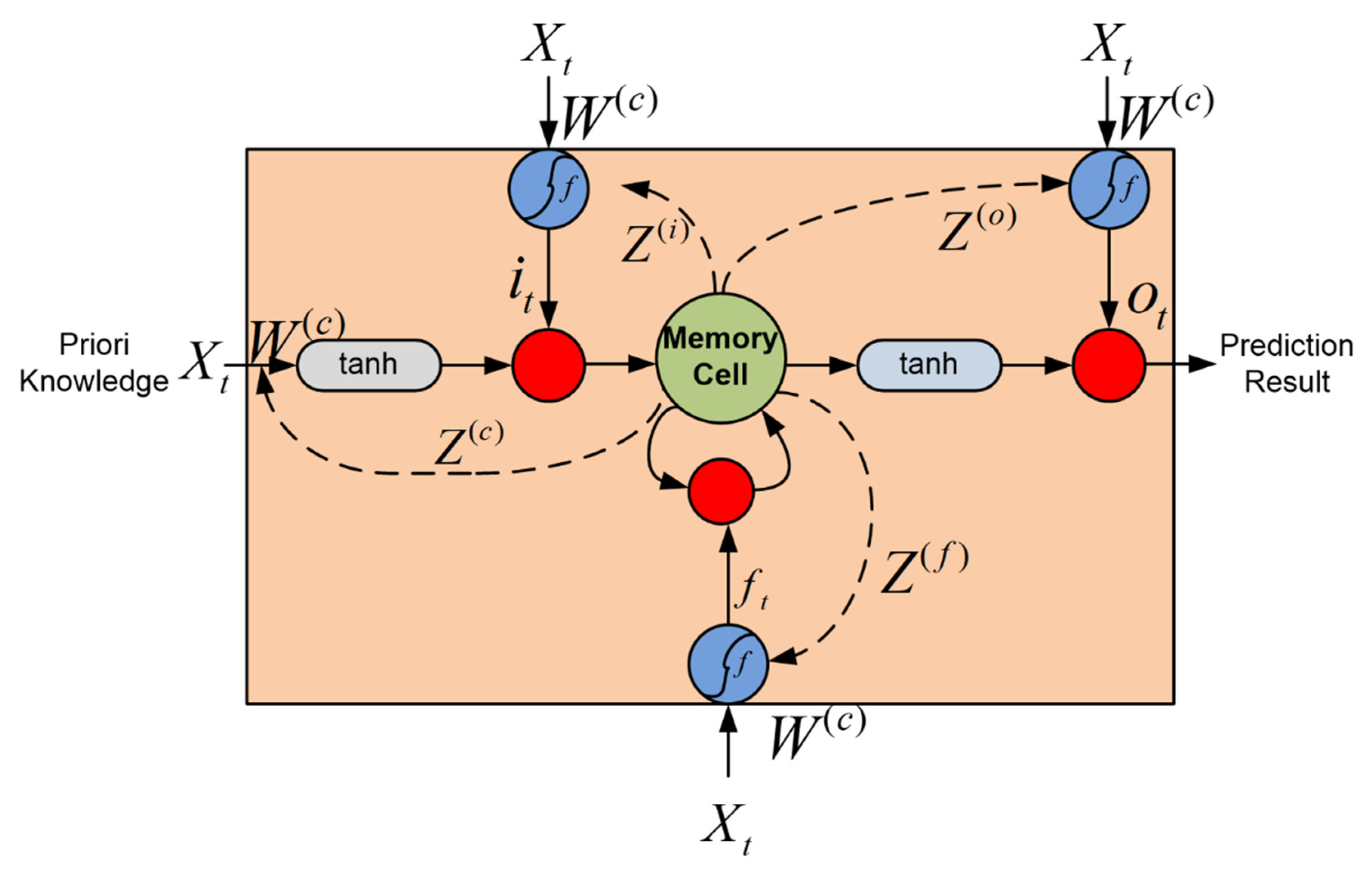
3.2. LSTM
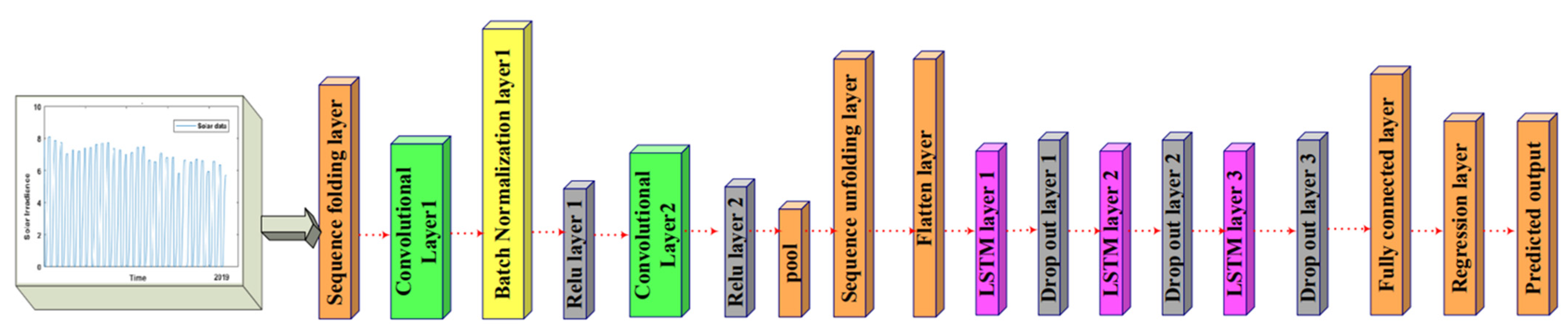
3.3. Proposed Multistep CNN-Stacked LSTM Model
4. Result and Analysis
4.1. Model Performance Measure
- (a)
- Mean Absolute Error (MAE): The MAE has been frequently utilized to solve regression problems and to examine forecast performance in the renewable energy industry. It is the absolute value of the difference between the forecast value and the observed value.
- (b)
- Root Mean Square Error (RMSE): The RMSE is the square root of the average of squared differences between forecast and observed values. RMSE is given by:
- (c)
- Mean Absolute Percentage Error (MAPE): It is the mean or average of the absolute percentage errors of forecasts.
- (d)
- Coefficient of Determination (): The Coefficient of Determination measures the extent that variability in the forecast errors is explained by variability in the observed values. The formula is as follows.where is the mean value of observations. When the value is close to one, the predicting accuracy improves.
- (e)
- Mean Squared Error (MSE): It measures the average of the squares of the errors and is given by,
- (f)
- Normalized Root Mean Squared Error (NRMSE): The NRMSE is the normalized form of the RMSE.
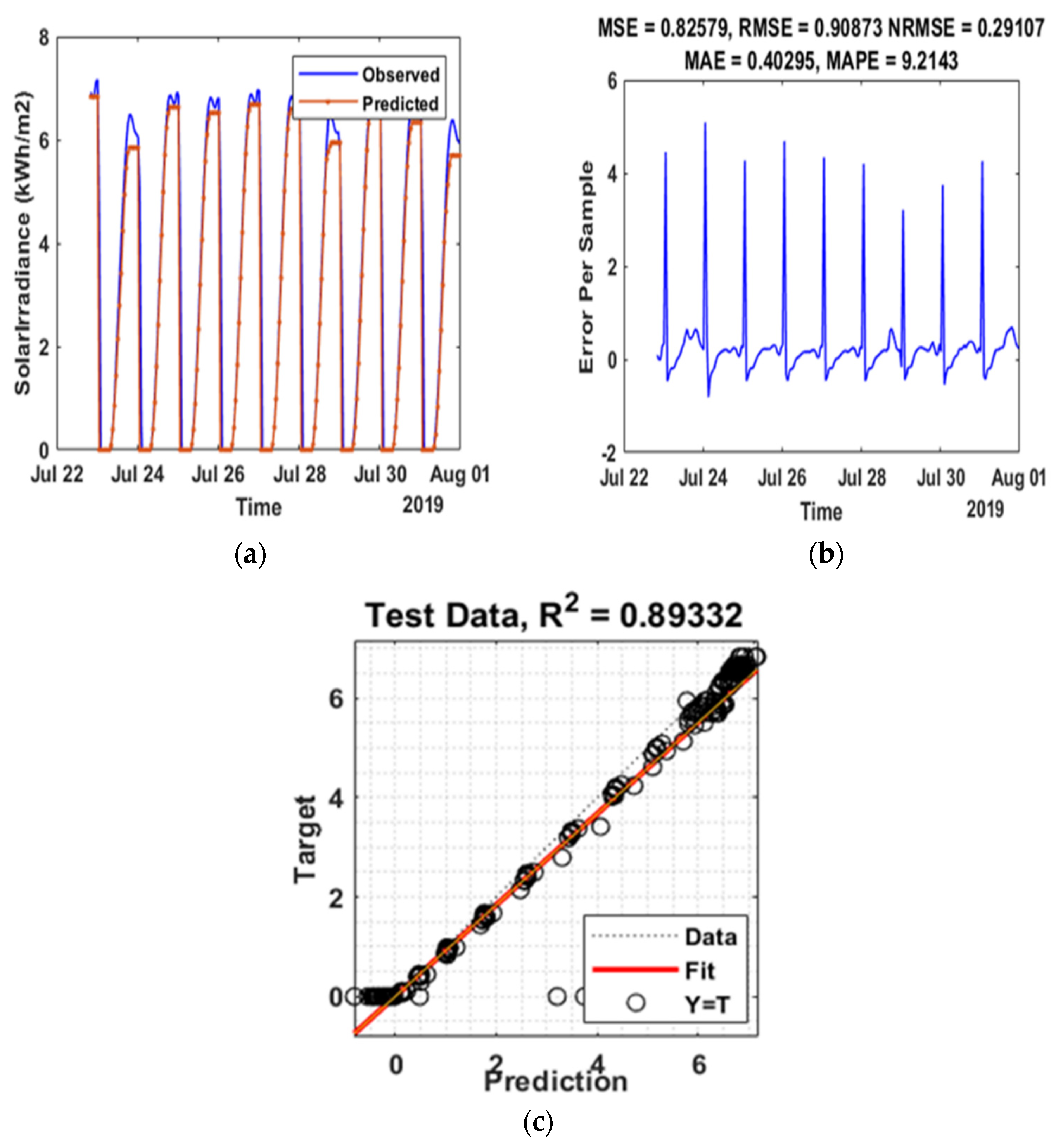
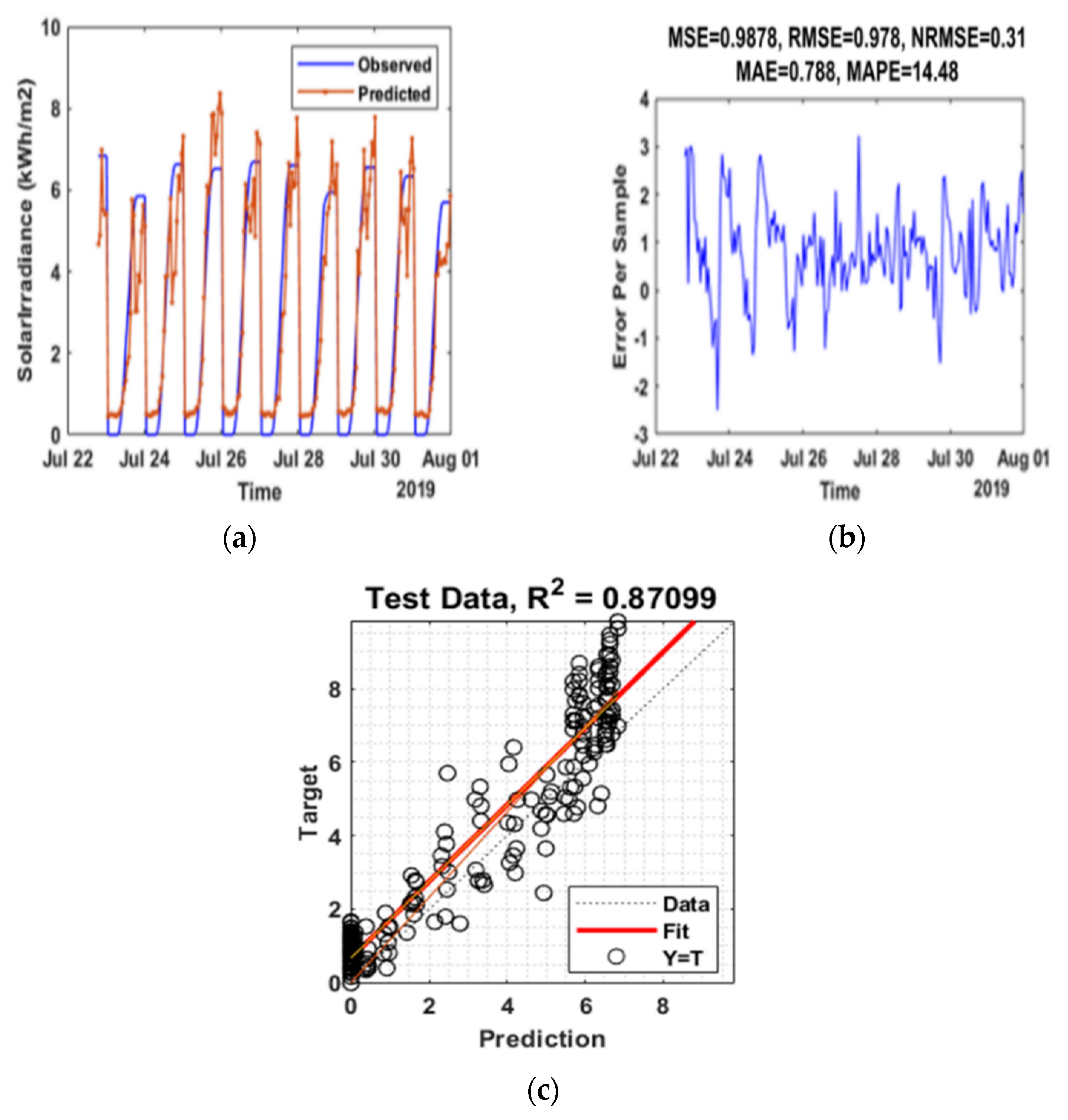
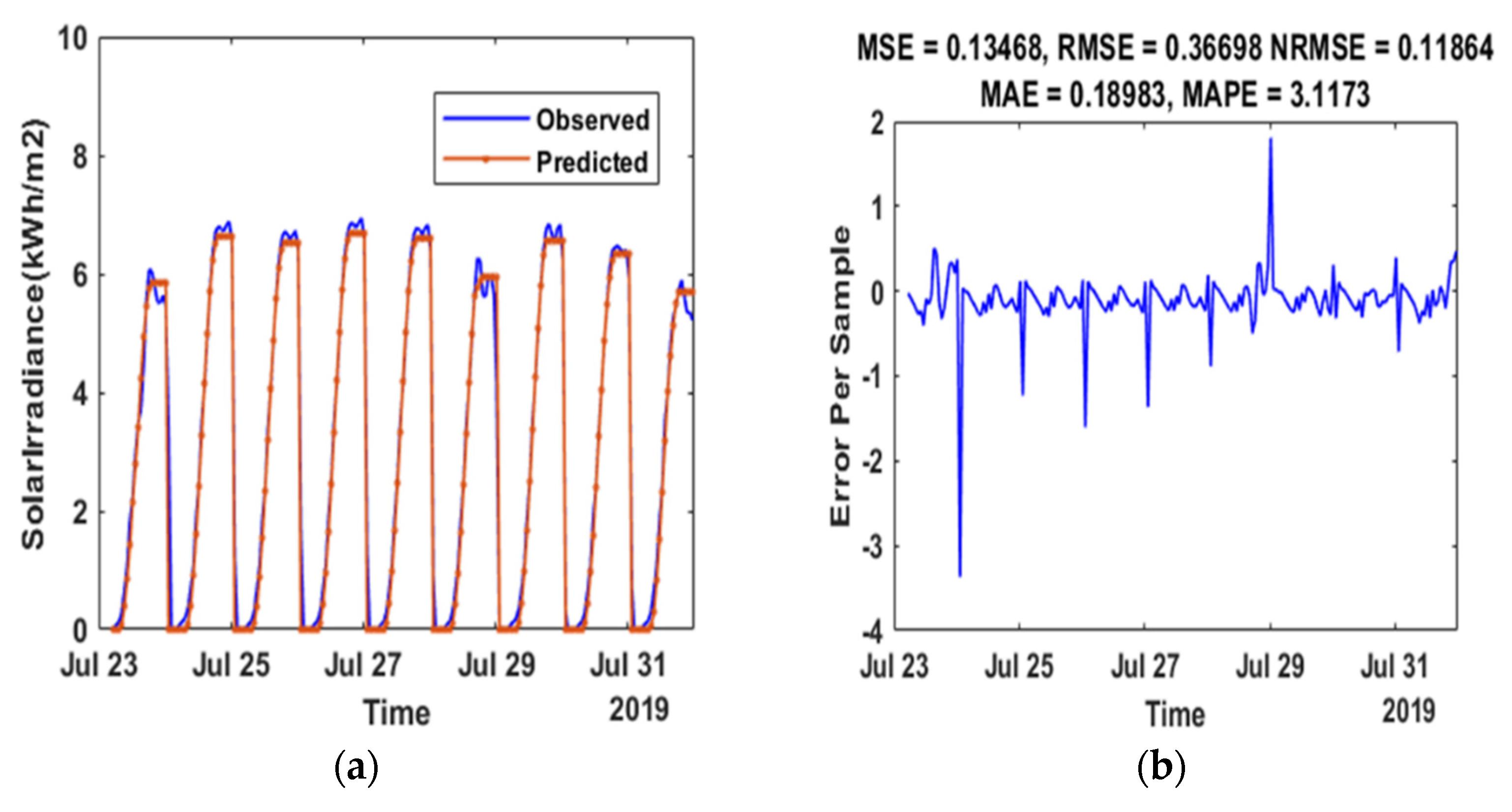
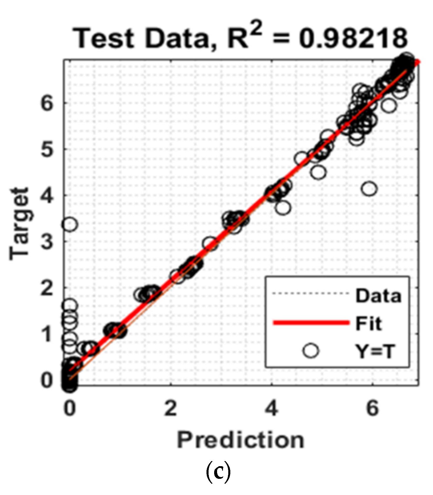
4.2. Case Study-I: Solar Irradiance-Sweihan Photovoltaic Independent Power Project, Abu Dhabi
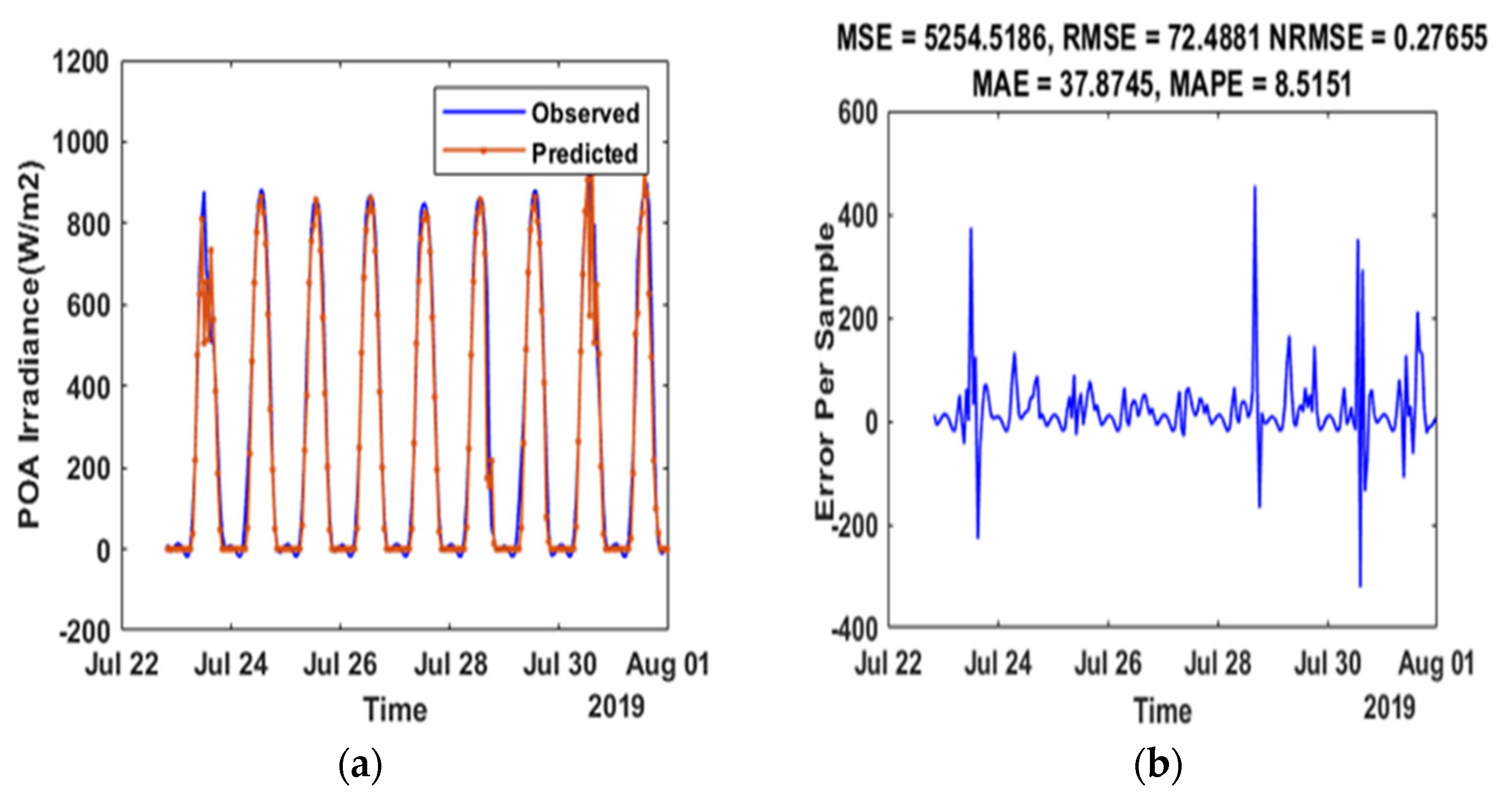
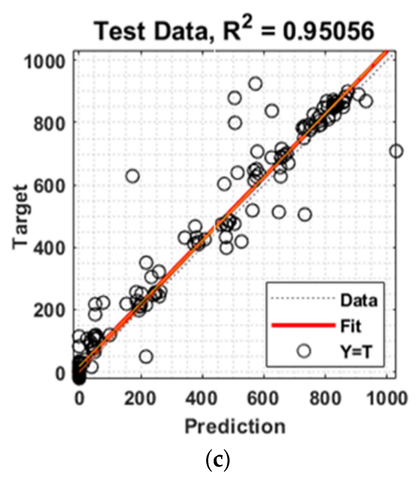
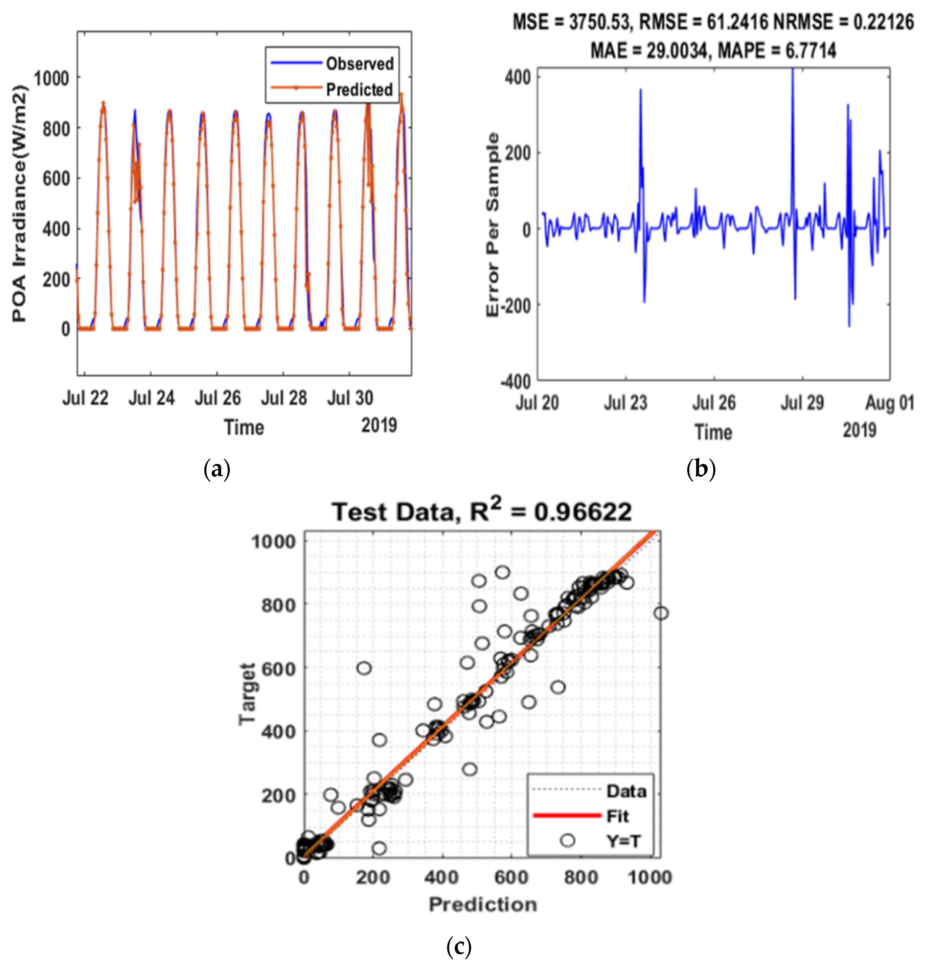
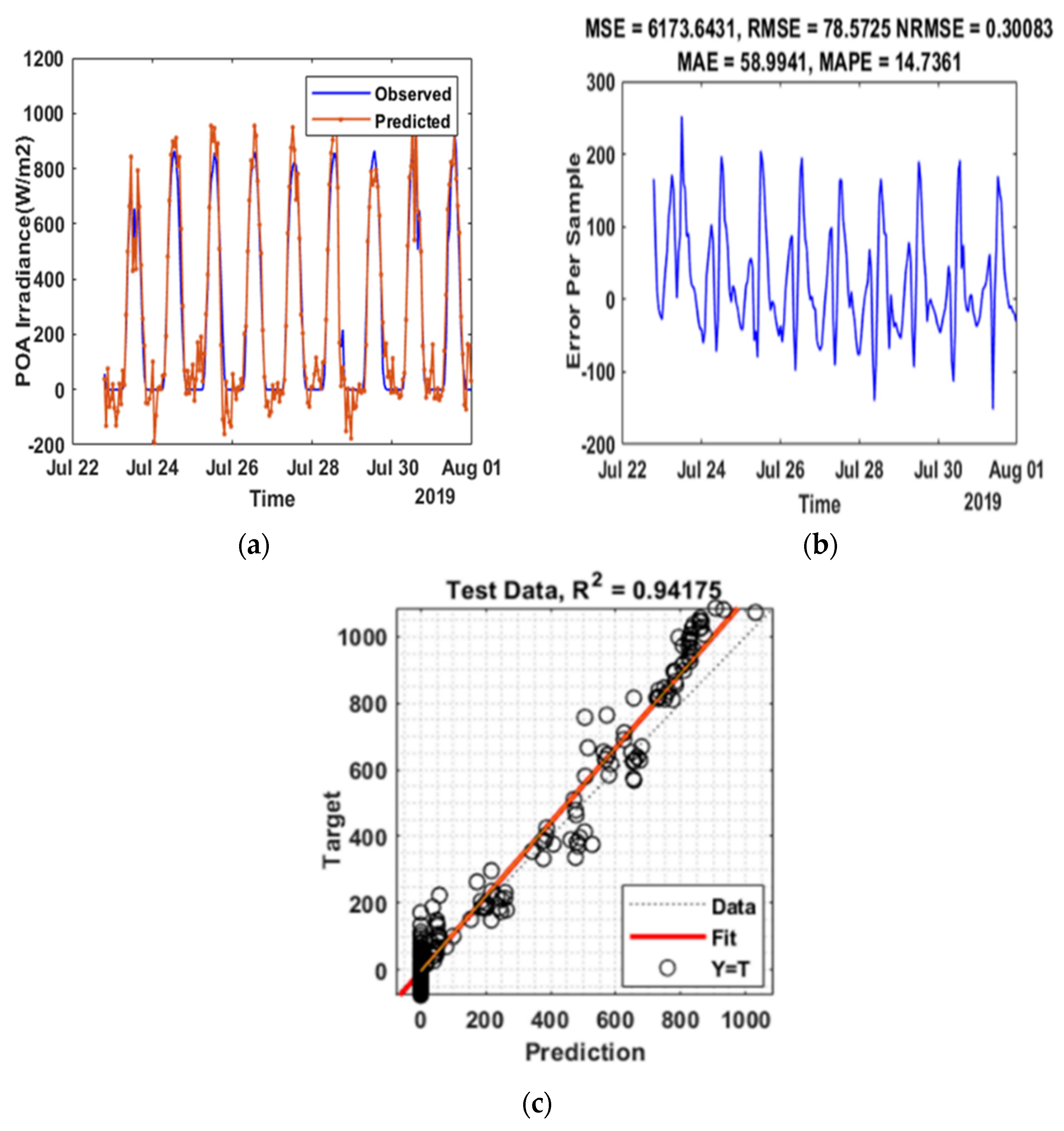
4.3. Case Study-II: POA_Sweihan Photovoltaic Independent Power Project, Abu Dhabi
4.4. Critical Analysis
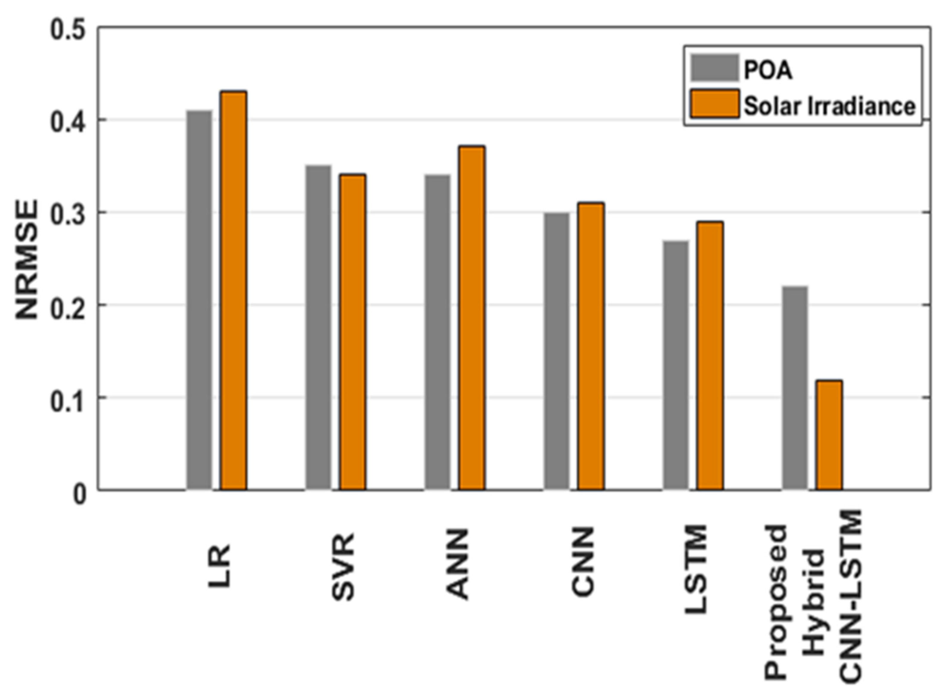
4.4.1. Comparative Analysis with the State-of-the-Art Techniques
4.4.2. Robustness of the Proposed Architecture under Noise-Injected Data
5. Conclusions
Author Contributions
Funding
Institutional Review Board Statement
Informed Consent Statement
Acknowledgments
Conflicts of Interest
Abbreviations
| ANN | Artificial Neural Network |
| CNN | Convolutional Neural Network |
| CSO | Chicken Swarm Optimization |
| DBN | Deep Belief Network |
| DCNN | Deep Convolutional Neural Network |
| DL | Deep Learning |
| ELM | Extreme Learning Machine |
| GHI | Global Horizontal Irradiance |
| GWO | Grey Wolf Optimization |
| LR | Linear Regression |
| LSTM | Long-Short-Term-Memory Network |
| MAE | Mean Absolute Error |
| MAPE | Mean Absolute Percentage Error |
| ML | Machine Learning |
| MLP | Multi-Layer Perceptron |
| MSE | Mean Squared Error |
| NRME | Normalized Root Mean Squared Error |
| POA | Plane of Array |
| RES | Renewable Energy Sources |
| RMSE | Root Mean Square Error |
| RNN | Recurrent Neural Network |
| SLR | Supervised Learning Algorithm |
| SNR | Signal to Noise Ratio |
| SRRL | Solar Radiation Research Laboratory |
| SPR | Support Vector Regression |
| SPV | Solar Photo Voltaic |
| SVM | Support Vector Machine |
| SVR | Support Vector Regression |
References
- Swain, M.K.; Mishra, M.; Bansal, R.C.; Hasan, S. A Self-Powered Solar Panel Automated Cleaning System: Design and Testing Analysis. Electr. Power Compon. Syst. 2021, 49, 308–320. [Google Scholar] [CrossRef]
- Murdock, H.E.; Gibb, D.; Andre, T.; Sawin, J.L.; Brown, A.; Ranalder, L.; Collier, U.; Dent, C.; Epp, B.; Hareesh Kumar, C.; et al. Renewables 2021-Global Status Report. Available online: https://www.ren21.net/wp-content/uploads/2019/05/GSR2021_Full_Report.pdf (accessed on 8 February 2022).
- Carrière, T.; Amaro e Silva, R.; Zhuang, F.; Saint-Drenan, Y.-M.; Blanc, P. A New Approach for Satellite-Based Probabilistic Solar Forecasting with Cloud Motion Vectors. Energies 2021, 14, 4951. [Google Scholar] [CrossRef]
- Rana, M.; Koprinska, I.; Agelidis, V.G. Univariate and multivariate methods for very short-term solar photovoltaic power forecasting. Energy Convers. Manag. 2016, 121, 380–390. [Google Scholar] [CrossRef]
- Wang, H.; Yi, H.; Peng, J.; Wang, G.; Liu, Y.; Jiang, H.; Liu, W. Deterministic and probabilistic forecasting of photovoltaic power based on deep convolutional neural network. Energy Convers. Manag. 2017, 153, 409–422. [Google Scholar] [CrossRef]
- De Giorgi, M.G.; Congedo, P.M.; Malvoni, M.; Laforgia, D. Error analysis of hybrid photovoltaic power forecasting models: A case study of mediterranean climate. Energy Convers. Manag. 2015, 100, 117–130. [Google Scholar] [CrossRef]
- Alonso-Montesinos, J.; Batlles, F. Solar radiation forecasting in the short- and medium-term under all sky conditions. Energy 2015, 83, 387–393. [Google Scholar] [CrossRef]
- Ruhang, X. The restriction research for urban area building integrated grid-connected PV power generation potential. Energy 2016, 113, 124–143. [Google Scholar] [CrossRef]
- Voyant, C.; Notton, G.; Kalogirou, S.; Nivet, M.-L.; Paoli, C.; Motte, F.; Fouilloy, A. Machine learning methods for solar radiation forecasting: A review. Renew. Energy 2017, 105, 569–582. [Google Scholar] [CrossRef]
- Yagli, G.M.; Yang, D.; Srinivasan, D. Automatic hourly solar forecasting using machine learning models. Renew. Sustain. Energy Rev. 2019, 105, 487–498. [Google Scholar] [CrossRef]
- Mishra, M.; Nayak, J.; Naik, B.; Abraham, A. Deep learning in electrical utility industry: A comprehensive review of a decade of research. Eng. Appl. Artif. Intell. 2020, 96, 104000. [Google Scholar] [CrossRef]
- Yu, Y.; Cao, J.; Zhu, J. An LSTM Short-Term Solar Irradiance Forecasting Under Complicated Weather Conditions. IEEE Access 2019, 7, 145651–145666. [Google Scholar] [CrossRef]
- Yadav, A.P.; Kumar, A.; Behera, L. RNN Based Solar Radiation Forecasting Using Adaptive Learning Rate. In Proceedings of the Swarm, Evolutionary, and Memetic Computing, Chennai, India, 19–21 December 2013; Springer: Cham, Switzerland, 2013; pp. 442–452. [Google Scholar]
- El Alani, O.; Abraim, M.; Ghennioui, H.; Ghennioui, A.; Ikenbi, I.; Dahr, F.E. Short term solar irradiance forecasting using sky images based on a hybrid CNN–MLP model. Energy Rep. 2021, 7, 888–900. [Google Scholar] [CrossRef]
- Dairi, A.; Harrou, F.; Sun, Y.; Khadraoui, S. Short-Term Forecasting of Photovoltaic Solar Power Production Using Variational Auto-Encoder Driven Deep Learning Approach. Appl. Sci. 2020, 10, 8400. [Google Scholar] [CrossRef]
- Huang, C.-J.; Kuo, P.-H. Multiple-Input Deep Convolutional Neural Network Model for Short-Term Photovoltaic Power Forecasting. IEEE Access 2019, 7, 74822–74834. [Google Scholar] [CrossRef]
- Li, L.-L.; Cheng, P.; Lin, H.-C.; Dong, H. Short-term output power forecasting of photovoltaic systems based on the deep belief net. Adv. Mech. Eng. 2017, 9, 1687814017715983. [Google Scholar] [CrossRef] [Green Version]
- Zhao, X.; Wei, H.; Wang, H.; Zhu, T.; Zhang, K. 3D-CNN-based feature extraction of ground-based cloud images for direct normal irradiance prediction. Sol. Energy 2019, 181, 510–518. [Google Scholar] [CrossRef]
- Zhu, T.; Guo, Y.; Li, Z.; Wang, C. Solar Radiation Prediction Based on Convolution Neural Network and Long Short-Term Memory. Energies 2021, 14, 8498. [Google Scholar] [CrossRef]
- Alharbi, F.R.; Csala, D. Wind Speed and Solar Irradiance Prediction Using a Bidirectional Long Short-Term Memory Model Based on Neural Networks. Energies 2021, 14, 6501. [Google Scholar] [CrossRef]
- Abdel-Nasser, M.; Mahmoud, K. Accurate photovoltaic power forecasting models using deep LSTM-RNN. Neural Comput. Appl. 2019, 31, 2727–2740. [Google Scholar] [CrossRef]
- Wen, L.; Zhou, K.; Yang, S.; Lu, X. Optimal load dispatch of community microgrid with deep learning based solar power and load forecasting. Energy 2019, 171, 1053–1065. [Google Scholar] [CrossRef]
- Zang, H.; Cheng, L.; Ding, T.; Cheung, K.W.; Liang, Z.; Wei, Z.; Sun, G. Hybrid method for short-term photovoltaic power forecasting based on deep convolutional neural network. IET Gener. Transm. Distrib. 2018, 12, 4557–4567. [Google Scholar] [CrossRef]
- Aprillia, H.; Yang, H.-T.; Huang, C.-M. Short-Term Photovoltaic Power Forecasting Using a Convolutional Neural Network–Salp Swarm Algorithm. Energies 2020, 13, 1879. [Google Scholar] [CrossRef]
- Zhong, J.; Liu, L.; Sun, Q.; Wang, X. Prediction of Photovoltaic Power Generation Based on General Regression and Back Propagation Neural Network. Energy Procedia 2018, 152, 1224–1229. [Google Scholar] [CrossRef]
- Lima, M.A.F.; Carvalho, P.C.; Fernández-Ramírez, L.M.; Braga, A.P. Improving solar forecasting using Deep Learning and Portfolio Theory integration. Energy 2020, 195, 117016. [Google Scholar] [CrossRef]
- Jayalakshmi, N.; Shankar, R.; Subramaniam, U.; Baranilingesan, I.; Karthick, A.; Stalin, B.; Rahim, R.; Ghosh, A. Novel Multi-Time Scale Deep Learning Algorithm for Solar Irradiance Forecasting. Energies 2021, 14, 2404. [Google Scholar] [CrossRef]
- Liebermann, S.; Um, J.-S.; Hwang, Y.; Schlüter, S. Performance Evaluation of Neural Network-Based Short-Term Solar Irradiation Forecasts. Energies 2021, 14, 3030. [Google Scholar] [CrossRef]
- Krizhevsky, A.; Sutskever, I.; Hinton, G.E. ImageNet Classification with Deep Convolutional Neural Networks. 2012. Available online: https://proceedings.neurips.cc/paper/2012/hash/c399862d3b9d6b76c8436e924a68c45b-Abstract.html (accessed on 8 February 2022).
- Yan, R.; Liao, J.; Yang, J.; Sun, W.; Nong, M.; Li, F. Multi-hour and multi-site air quality index forecasting in Beijing using CNN, LSTM, CNN-LSTM, and spatiotemporal clustering. Expert Syst. Appl. 2021, 169, 114513. [Google Scholar] [CrossRef]
- Husein, M.; Chung, I.-Y. Day-Ahead Solar Irradiance Forecasting for Microgrids Using a Long Short-Term Memory Recurrent Neural Network: A Deep Learning Approach. Energies 2019, 12, 1856. [Google Scholar] [CrossRef] [Green Version]
- Zhao, Z.; Chen, W.; Wu, X.; Chen, P.C.Y.; Liu, J. LSTM network: A deep learning approach for short-term traffic forecast. IET Intell. Transp. Syst. 2017, 11, 68–75. [Google Scholar] [CrossRef] [Green Version]
- Barzegar, R.; Aalami, M.T.; Adamowski, J. Short-term water quality variable prediction using a hybrid CNN–LSTM deep learning model. Stoch. Hydrol. Hydraul. 2020, 34, 415–433. [Google Scholar] [CrossRef]
- Gao, B.; Huang, X.; Shi, J.; Tai, Y.; Zhang, J. Hourly forecasting of solar irradiance based on CEEMDAN and multi-strategy CNN-LSTM neural networks. Renew. Energy 2020, 162, 1665–1683. [Google Scholar] [CrossRef]
- Chen, Y.; Wang, Y.; Dong, Z.; Su, J.; Han, Z.; Zhou, D.; Zhao, Y.; Bao, Y. 2-D regional short-term wind speed forecast based on CNN-LSTM deep learning model. Energy Convers. Manag. 2021, 244, 114451. [Google Scholar] [CrossRef]
- Tian, C.; Ma, J.; Zhang, C.; Zhan, P. A Deep Neural Network Model for Short-Term Load Forecast Based on Long Short-Term Memory Network and Convolutional Neural Network. Energies 2018, 11, 3493. [Google Scholar] [CrossRef] [Green Version]
- Massaoudi, M.; S Refaat, S.; Abu-Rub, H.; Chihi, I.; Oueslati, F.S. PLS-CNN-BiLSTM: An end-to-end algorithm-based Savitzky–Golay smoothing and evolution strategy for load forecasting. Energies 2020, 13, 5464. [Google Scholar] [CrossRef]
- Srivastava, N.; Hinton, G.; Krizhevsky, A.; Sutskever, I.; Salakhutdinov, R. Dropout: A simple way to prevent neural networks from overfitting. J. Mach. Learn. Res. 2014, 15, 1929–1958. [Google Scholar]
- Montgomery, D.C.; Peck, E.A.; Vining, G.G. Introduction to Linear Regression Analysis; John Wiley & Sons: Hoboken, NJ, USA, 2021. [Google Scholar]
- Awad, M.; Khanna, R. Support vector regression. In Efficient Learning Machines; Apress: Berkeley, CA, USA, 2015; pp. 67–80. [Google Scholar]
- Maldonado, S.; González, A.; Crone, S. Automatic time series analysis for electric load forecasting via support vector regression. Appl. Soft Comput. 2019, 83, 105616. [Google Scholar] [CrossRef]
- Najeebullah; Zameer, A.; Khan, A.; Javed, S.G. Machine Learning based short term wind power prediction using a hybrid learning model. Comput. Electr. Eng. 2015, 45, 122–133. [Google Scholar] [CrossRef]
- Hong, Y.-Y.; Martinez, J.J.F.; Fajardo, A.C. Day-Ahead Solar Irradiation Forecasting Utilizing Gramian Angular Field and Convolutional Long Short-Term Memory. IEEE Access 2020, 8, 18741–18753. [Google Scholar] [CrossRef]
- Li, G.; Xie, S.; Wang, B.; Xin, J.; Li, Y.; Du, S. Photovoltaic Power Forecasting with a Hybrid Deep Learning Approach. IEEE Access 2020, 8, 175871–175880. [Google Scholar] [CrossRef]
- Kumar, D.; Mathur, H.D.; Bhanot, S.; Bansal, R.C. Forecasting of solar and wind power using LSTM RNN for load frequency control in isolated microgrid. Int. J. Model. Simul. 2021, 41, 311–323. [Google Scholar] [CrossRef]
- Feng, C.; Zhang, J. SolarNet: A sky image-based deep convolutional neural network for intra-hour solar forecasting. Sol. Energy 2020, 204, 71–78. [Google Scholar] [CrossRef]
- Zang, H.; Liu, L.; Sun, L.; Cheng, L.; Wei, Z.; Sun, G. Short-term global horizontal irradiance forecasting based on a hybrid CNN-LSTM model with spatiotemporal correlations. Renew. Energy 2020, 160, 26–41. [Google Scholar] [CrossRef]
- Agga, A.; Abbou, A.; Labbadi, M.; El Houm, Y. Short-term self consumption PV plant power production forecasts based on hybrid CNN-LSTM, ConvLSTM models. Renew. Energy 2021, 177, 101–112. [Google Scholar] [CrossRef]
- Kumari, P.; Toshniwal, D. Long short term memory–convolutional neural network based deep hybrid approach for solar irradiance forecasting. Appl. Energy 2021, 295, 117061. [Google Scholar] [CrossRef]
- Singh, S. Noise impact on time-series forecasting using an intelligent pattern matching technique. Pattern Recognit. 1999, 32, 1389–1398. [Google Scholar] [CrossRef]
- Sarp, S.; Kuzlu, M.; Cali, U.; Elma, O.; Guler, O. Analysis of False Data Injection Impact on AI-based Solar Photovoltaic Power Generation Forecasting. arXiv 2021, arXiv:2110.09948. [Google Scholar] [CrossRef]


| Ref. | Year | Method | Data Used | Performance Metrics |
|---|---|---|---|---|
| [19] | 2021 | SCNN–LSTM | NREL’s Solar Radiation Research Laboratory (SRRL) | NRMSE = 23.47% nMAE = 13.75% |
| [21] | 2019 | LSTM–RNN | Aswan (Dataset1) and Cairo (Dataset2) cities, Egypt. | 82.15 (RMSE) |
| [22] | 2019 | DRNN–LSTM | Sails in the Desert, Yulara, Australia. | DRNN–LSTM: 7.53 (RMSE), 4.369 (MAE), 15.87% (MAPE) |
| [23] | 2018 | VMD–CNN | An electric power company in Jiangsu Province, China. | 1.5418 (MAPE), 2.0533 (RMSE), 0.1752 (MAE) |
| [24] | 2020 | CNN LSTM | Data is taken from 500 kWp PV plant in Taiwan [25] | CNN: 29.72% (MAPE), 2.94% (MRE) and for LSTM: 35.85% (MAPE), 5.99% (MRE). |
| [26] | 2020 | LSTM | Datset1: Brazilian data Datset2: Spanish data | MAPE: 7.19% (LSTM) |
| [27] | 2021 | Hybrid CSO (Chicken Swarm Optimization)-GWO (Grey Wolf Optimization) | The Photo-Voltaic Graphical Information System—Surface Solar Radiation Dataset Heliosat (PVGIS-SARAH) | R2 = 0.9731 |
| [28] | 2021 | Hybrid LSTMconv | www.soda-pro.com (accessed on 21 May 2021) | MAE = 66.75%(ULM) MAE = 62.87%(Hull) |
| No. | Layer | Function |
|---|---|---|
| 1 | Sequence Input Layer | Inputs sequence data to a network. |
| 2 | Sequence Folding Layer | The batch of data sequences is transformed into a batch of data |
| 3 | Convolution2dLayer | Sliding filters are applied to the input. |
| 4 | Relu Layer | Every element of the input is subjected to a threshold operation. |
| 5 | averagePooling2dLayer | Down samples the input by splitting it into rectangular pooling zones and calculating the average values of each. |
| 6 | Sequence Unfolding Layer | Re-establish the input data’s sequence architecture after the sequence folding layer. |
| 7 | Flatten layer | A flatten layer reduces the input’s spatial size to the channel size. |
| 8 | LSTM layer | In time-series data, the LSTM layer acquires long-term dependencies between time steps. |
| 9 | Drop out layer | With a certain probability, the dropout layer transforms input elements to zero randomly. |
| 10 | Fully Connected Layer | A fully connected layer outputs the prediction |
| 11 | Regression Layer | Evaluate the half-mean-squared-error loss. |
| Group | Parameter | Value | Description |
|---|---|---|---|
| Sequence folding layer | |||
| Conv2DLayer 1 | filters | 256 | Filter size = 5 × 5 |
| Batch normalization layer | |||
| Relu layer | |||
| Conv2DLayer 2 | filters | 256 | Filter size = 5 × 5 |
| Averagepoolng2D layer | Filter size = 5 × 5 | ||
| Sequence unfolding layer | |||
| Flatten layer | |||
| LSTM layer1 | No: of hidden units = 100 | Drop out = 0.1 | |
| LSTM layer2 | No: of hidden units = 100 | Drop out = 0.1 | |
| LSTM layer3 | No: of hidden units = 300 | Drop out = 0.1 | |
| Fully connected layer | |||
| Regression layer | |||
| Training | Optimizer | ADAM optimizer | |
| Training | Mini batch size | 64 | |
| Training | Learning rate | 0.00501 | Learning rate of optimizer |
| Architecture | RMSE | MAE | MAPE | MSE | NRMSE | |
|---|---|---|---|---|---|---|
| CNN | 0.98 | 0.78 | 14.48 | 0.87 | 0.99 | 0.31 |
| LSTM | 0.90 | 0.40 | 9.20 | 0.90 | 0.82 | 0.29 |
| Multi step CNN Stacked LSTM | 0.36 | 0.18 | 3.11 | 0.98 | 0.13 | 0.11 |
| Architecture | RMSE | MAE | MAPE | MSE | NRMSE | |
|---|---|---|---|---|---|---|
| CNN | 78.50 | 58.90 | 14.70 | 0.94 | 6173 | 0.30 |
| LSTM | 72.40 | 38.00 | 9.00 | 0.95 | 5254 | 0.27 |
| Multi step CNN Stacked LSTM | 61.24 | 29.00 | 6.70 | 0.96 | 3750 | 0.22 |
| Ref. | Year | Method | Country | Lowest Error |
|---|---|---|---|---|
| [16] | 2019 | DNN models (LSTM, CNN) | Taiwan | RMSE = 126.91–140.9 |
| [21] | 2017 | 5 different LSTM architectures | Egypt | RMSE: 82.15–136.87 |
| [34] | 2020 | CEEMDAN-CNN-LSTM | Los Anegles | RMSE = 34.72 NRMSE = 12.19 |
| [43] | 2020 | DNN models (LSTM, CNN LSTM, Conv LSTM) | Fuhai, Taiwan | R2 = 0.54–0.7 RMSE = 0.18–0.2 |
| [44] | 2020 | Hybrid LSTM | Limberg, Belgium | RMSE = 6.4 R2 = 0.95–0.98 |
| [45] | 2020 | LSTM | Gujarat, India | RMSE = 11.6 |
| [46] | 2020 | Solar Net model (Deep CNN) | Golden Colerado | RMSE = 116.82 NRMSE = 8.85% |
| [47] | 2020 | CNN-LSTM | Dallas | RMSE = 97.10 NRMSE = 24.53 |
| [48] | 2021 | CNN-LSTM | Morocco | RMSE = 8.6 |
| [49] | 2021 | LSTM-CNN | San Diego | RMSE = 42.89 |
| Proposed work: Multistep CNN Stacked LSTM | Abu Dhabi | NRMSE = 0.11 RMSE = 0.36 | ||
| Error Metrics | 0% (No Noise Is Injected) | 50% (Noise Injected to 50% of Data) | 100% (Noise Injected to 100% of Data) |
|---|---|---|---|
| RMSE | 0.36 | 0.3670 | 0.3930 |
| MAE | 0.18 | 0.1898 | 0.1922 |
| MAPE | 3.11 | 3.1173 | 2.8315 |
| R2 | 0.98 | 0.9822 | 0.9795 |
| MSE | 0.13 | 0.1347 | 0.1545 |
| NRMSE | 0.11 | 0.1186 | 0.1260 |
| Error Metrics | 0% (No Noise Is Injected) | 50% (Noise Injected to 50% of Data) | 100% (Noise Injected to 100% of Data) |
|---|---|---|---|
| RMSE | 0.36 | 0.367 | 0.75 |
| MAE | 0.18 | 0.189 | 0.41 |
| MAPE | 3.11 | 3.11 | 6.19 |
| R2 | 0.98 | 0.98 | 0.93 |
| MSE | 0.13 | 0.1347 | 0.57 |
| NRMSE | 0.11 | 0.1186 | 0.23 |
Publisher’s Note: MDPI stays neutral with regard to jurisdictional claims in published maps and institutional affiliations. |
© 2022 by the authors. Licensee MDPI, Basel, Switzerland. This article is an open access article distributed under the terms and conditions of the Creative Commons Attribution (CC BY) license (https://creativecommons.org/licenses/by/4.0/).
Share and Cite
Elizabeth Michael, N.; Mishra, M.; Hasan, S.; Al-Durra, A. Short-Term Solar Power Predicting Model Based on Multi-Step CNN Stacked LSTM Technique. Energies 2022, 15, 2150. https://doi.org/10.3390/en15062150
Elizabeth Michael N, Mishra M, Hasan S, Al-Durra A. Short-Term Solar Power Predicting Model Based on Multi-Step CNN Stacked LSTM Technique. Energies. 2022; 15(6):2150. https://doi.org/10.3390/en15062150
Chicago/Turabian StyleElizabeth Michael, Neethu, Manohar Mishra, Shazia Hasan, and Ahmed Al-Durra. 2022. "Short-Term Solar Power Predicting Model Based on Multi-Step CNN Stacked LSTM Technique" Energies 15, no. 6: 2150. https://doi.org/10.3390/en15062150
APA StyleElizabeth Michael, N., Mishra, M., Hasan, S., & Al-Durra, A. (2022). Short-Term Solar Power Predicting Model Based on Multi-Step CNN Stacked LSTM Technique. Energies, 15(6), 2150. https://doi.org/10.3390/en15062150