Waste Clothing Recycling Channel Selection Using a CoCoSo-D Method Based on Sine Trigonometric Interaction Operational Laws with Pythagorean Fuzzy Information

Abstract

Under the influence of circular economy theory, waste clothing recycling has been widely studied in the resource sector, and the waste clothing recycling channel (WCRC) is the vital link that affects the recycling efficiency of waste clothing. How to select the optimal WCRC is considered a typical multiple attribute group decision-making (MAGDM) problem. In this article, we develop sine trigonometric interaction operational laws (IOLs) (STIOLs) using Pythagorean fuzzy information. The sine trigonometric interaction Pythagorean fuzzy weighted averaging (STI-PyFWA) and sine trigonometric interaction Pythagorean fuzzy weighted geometric (STI-PyFWG) operators are advanced, and their several desirable properties are discussed. Further, we build a MAGDM framework based on the modified Pythagorean fuzzy CoCoSo (Combined Compromise Solution) method to solve the WCRC selection problem. The combined weight of attributes is determined, and the proposed aggregation operators (AOs) are applied to the CoCoSo method. A Pythagorean fuzzy distance measure is used to achieve the defuzzification of aggregation strategies. Finally, we deal with the WCRC selection problem for a sustainable environment by implementing the proposed method and performing sensitivity analysis and comparative study to validate its effectiveness and superiority.

1. Introduction

With the development of the global economy, the average wear times of clothing are decreasing, and their service cycle is shortening year by year under the combined action of fast consumption, pursuing fashion and other factors [1]. The rapid growth of discarded clothing indicates that it has become a new solid waste and has a negative impact on the environment [2]. Global clothing and footwear consumption continues to grow at an annual rate of 3.4% from 62 million tons from 2015, according to GFA (Global Fashion Agenda) and UNEP (United Nations Environment Programme), while the recovery rate of textile waste is only around 12% [3,4]. In order to solve the negative consequences in terms of discarded clothing, the government, commercial practitioners, and academic researchers believe that the circular economy is the key to handling the problem [5].

In recent years, compared with the “take-make-use-dispose” system of a linear economy, the concept of a circular economy has gradually been paid attention in the clothing industry, and some plans and implementation strategies have been developed to make the fashion-related economy more circular. A new concept of “circular fashion” has emerged in the industry [6,7]. In practice, the circular fashion business strategy depends on three main principles, including “designing out waste and pollution” in the production stage, “keeping fashion products and their materials in longer and continuous use” in the use stage, and requiring enterprises to seek “regenerate natural systems” in the business strategy [8,9]. In general, renewable resource plants collect waste clothes from consumers through various recycling channels. The plants classify waste clothes according to certain standards and produce new clothes products of different forms to present consumers again through the process of redress, reuse and remanufacturing. This closed-loop process is called the circulation of waste clothing. As shown in Figure 1.

In this process, the recycling channel is a vital link that cannot be ignored. The design, layout and operation efficiency of waste clothing recycling channels can directly affect the quantity and speed of waste clothing disposal. In the UK, the most effective recycling channels are social welfare organizations and second-hand clothing banks, which collect 230,000 tons a year. However, compared with about 9 million tons of waste clothes, the strength and effect of recycling are not worth mentioning [10]. In China, nearly 100 million tons of waste textiles every year are produced in production and consumption, but the reuse rate is less than 14% [11]. On the other hand, the textile industry suffers from a tight supply of raw materials in China, with imports of over 65%. As most used clothing has the potential to be reused or recycled, the Chinese government announced 85 major demonstration projects for national resource recycling in 2016, including used textiles. Several ways of recycling waste clothes have emerged in Chinese society under the stimulation of the market economy and the encouragement of the government, including collection projects carried out by local governments or non-business organizations, charitable donation activities carried out by non-business organizations, enterprises collecting brand waste clothes from consumers and carrying out online waste clothes recycling by using “Internet +” technology [12]. Currently, scholars are studying recycling channels from the perspective of consumer psychology or behavior [12], but there is no assessment and selection of WCRC from the perspective of enterprise investment to seek the most appropriate recycling channel. In the actual situation, some important issues need to be taken into account in the selection of WCRC. Therefore, the selection of an optimal WCRC can be regarded as a typical MAGDM problem.

1.1. Pythagorean Fuzzy Sets

An attribute evaluation value usually embraces ambiguous and impermeable information in MAGDM problems. However, as the actual group decision-making problem becomes more and more complex, scholars are faced with significant challenges in the expression of attribute variables. As an information representation method, fuzzy set (FS) [13] is widely applied to solve information modeling problems with vague and uncertain information in many fields, but the FS has only membership degree (MD) $M\left(x\right) (0\le M\left(x\right)\le 1)$, so it is difficult to comprehensively describe and depict the uncertainty degree of human’s cognition of things. In view of this, Atanassov [14] developed an intuitionistic fuzzy set (IFS), which uses the MD $M\left(x\right)$ and non-membership degree (ND) $N\left(x\right) \left(0\le N\left(x\right)\le 1\right)$ to describe more detailed information than the FS. The characteristic of IFS is $M\left(x\right)+N\left(x\right)\le 1$. In order to overcome the shortcoming that the IFS cannot be used in decision scenarios where the sum of $M\left(x\right)$ and $N\left(x\right)$ greater than one, Yager [15] originated the idea of the Pythagorean fuzzy set (PyFS), and its $M\left(x\right)$ and $N\left(x\right)$ meet the conditions: ${\left(M\left(x\right)\right)}^2+{\left(M\left(x\right)\right)}^2\le 1$. Therefore, the nature of vagueness and uncertainty of assessment information can be depicted by PyFS, which are better than IFS.

PyFS has been considered and favored by many scholars. The current study mainly focuses on AOs and sorting techniques. In the study of PyFS AOs, Wei [16] and Wei and Lu [17] developed several power AOs, and then some interaction AOs were proposed. Gao [18] used Hamacher operation and Prioritized AOs to develop Pythagorean fuzzy Hamacher Prioritized AOs. Wang and Li [19] extended power Bonferroni mean (PBM) with IOLs in the PyFSs and proposed Pythagorean fuzzy PBM (PyFIPBM) and weighted PyFIPBM operators. Wang et al. [20] explored various interactive Hamacher power AOs for PyFNs. Wei [21] investigated the Maclaurin symmetric mean (MSM) and its weighted form with PyFNs. In terms of sorting technique research, Chen [22] proposed VIKOR based on the remoteness index in PyFSs. Akram et al. [23] developed the ELECTRE I (Elimination and Choice Translating REality I) method to settle Pythagorean fuzzy MAGDM problems. The prospect theory-based TODIM approach was extended by Ren et al. [24] with Pythagorean fuzzy information. A VIKOR-based approach with PyFSs was advanced by Gul et al. [25] to assess the safety risk in the mine industry. Peng and Yang [26] integrated the Choquet integral (CI) AO with MABAC (multi-attributive border approximation area comparison) method to deal with MAGDM problems with PyFNs. The Pythagorean fuzzy hybrid TOPSIS and Pythagorean fuzzy hybrid ELECTRE I were aggregated by Akram et al. [27] to apply in FMEA. Peng and Ma [28] explored the CODAS (COmbinative Distance-based ASessment)-based Pythagorean fuzzy algorithm to solve the MADM problem. A prospect theory-based EDAS (Evaluation based on the Distance from Average Solution) approach was studied by Li et al. [29] in a Pythagorean fuzzy environment. The novel score function and distance measures were explored and contributed to the Pythagorean fuzzy MULTIMOORA method by Huang et al. [30]. The PROMETHEE (preference ranking organization method of enrichment evaluations) was extended by Zhang et al. [31] with PyFNs. The PROMETHEE method with PyFSs was applied by Molla et al. [32] to solve a medical diagnosis problem. The CPT-TODIM (cumulative prospect theory TODIM) method is proposed for Pythagorean fuzzy MAGDM issues by Zhao et al. [33]. To settle MAGDM problems, the Pythagorean fuzzy TOPSIS method was explored by Akram et al. [34]. Sarkar and Biswas [35] developed the Pythagorean fuzzy TOPSIS technique with a new distance measure for transportation management. The VIKOR method based on novel divergence and entropy measures of PyFNs was advanced by Rani et al. [36] to select renewable energy technologies. To evaluate sustainable suppliers, the Pythagorean fuzzy WASPAS method with a combination weighting technique was developed by Alrasheedi et al. [37]. Ayyildiz et al. [38] established a new framework with the Pythagorean fuzzy AHP-WASPAS method.

1.2. Operational Laws

The operational laws of fuzzy sets play a critical link in the process of evaluation information fusion. As we all know, the basic operation rules have been widely combined with various fuzzy theories for expansion and application. In addition, there are some operation rules with their own characteristics. One is some more generalized operation rules, such as exponential operation laws (EOLs) [39], logarithmic operation laws (LOLs) [40] and STOLs [41,42,43,44]. Compared with EOLs and LOLs, STOLs play a leading role during the fusion of information [41]. The main superiorities of STOLs are of periodicity and symmetricity about the origin, so they satisfy the DM’s preferences over the multi-time phase parameters [44]. Based on this, scholars have extended STOLs to a variety of fuzzy environments, such as q-ROFS (q-rung orthopair fuzzy set) [45], SFS (spherical fuzzy set) [41], PyFS [42,43], and SVNS (simple-valued neutrosophic set) [44]. In terms of IOLs, the IOLs [46] mainly consider the interaction between MD and ND in intuitionistic fuzzy numbers, and its main function is to eliminate the counterintuitive phenomenon and completely keep the vagueness and uncertainty of evaluation information, to make it consistent with the actual situation. Some scholars have extended IOLs in Pythagorean fuzzy environments and proposed various AOs [17,19,46,47,48,49,50,51]. However, there is no study on integrating STOLs and IOLs. Therefore, it is necessary to explore new STIOLs and investigate their desirable properties with PyFNs by integrating the respective strengths of STOLs and IOLs.

1.3. The ITARA Method

The weight of attributes plays a vital role in determining the optimal alternative by the MADM method. Generally, there are three methods to obtain attribute weight: subjective weighting method (e.g., DEMATEL (Decision-making trial and evaluation laboratory), ANP (Analytic Network Process), BWM (Best-Worst Method), AHP (Analytical Hierarchy Process), etc.), objective weighting method (e.g., maximum deviation, Entropy weighting and CRITIC (Criteria importance through inter-criteria correlation), etc.) and the objective combination of subjective and objective. The ITARA is a new approach for assigning semi-objective weight to attributes proposed by Hatefi [52]. This method extracts almost similar attribute values from the performance data of existing alternatives based on decentralized logic and assigns small weights to attributes [53,54]. The ITARA method has been widely used in recent years. Liu et al. [53] extended the ITARA method in q-RONFNs (normal q-rung orthopair fuzzy numbers) environment to obtain attribute weight. Chang et al. [54] added the concept of aspiration level to the ITARA method for attribute weight of sustainable supplier evaluation in the electronic manufacturing industry. Alper Sofuoğlu [55] applied the ITARA-based decision technique to deal with the problem of material selection of flywheels. The ITARA approach was applied by Du et al. [56] to obtain the weight of attributes in an intuitionistic normal cloud environment. Gong et al. [57] extended the ITARA approach to calculate attribute weight in q-ROFSs (q-rung orthopair fuzzy sets) environment. To select stackers in logistics systems, the ITRATA and MARCOS (Measurement of alternatives and Ranking according to compromise solution) were integrated by Ulutas et al. [58]. The improved ITARA approach was utilized by Lo et al. [59] to determine reliable weights. To assess e-learning websites, the ITARA approach was extended with linguistic hesitation fuzzy sets by Gong et al. [60]. The ITARA approach was extended by Liu et al. [61] in a linguistic spherical fuzzy environment.

1.4. The CoCoSo Method

Over the years, some alternative ranking techniques have made significant contributions to the development of various rational decision theories. However, due to the limitations of human cognition, the uncertainty of information, and the pressure of time, DMs generally use bounded rationality in practical decision-making activities. An appropriate decision-making tool is needed to deal with these issues. The CoCoSo method [62] is a decision-making technique based on combinatorial and compromise perspectives. By integrating the values of WSM (weighted sum model) and WPM (weighted power model) models with different aggregation strategies, a compromise solution has been obtained. In this way, internal equilibrium can be achieved, which has the advantages of avoiding decision-making compensatory problems and achieving final utility. Moreover, the computational complexity is relatively low. At present, CoCoSo has been extensively used in different group decision environments, such as fuzzy numbers [63], PyFNs [64,65], q-ROFNs [66], grey number [67] and rough number [68,69], and has been applied to different fields. Its research status is listed in

Table 1. Research status of existing CoCoSo methods for group decision making problems.

Refs.	Type of Info.	DMs’ Weight	Weight of Attribute			OLs	Defuzzification		Application Area
			Subjective	Objective	Combined		Approach	Step in CoCoSo
Erceg et al. (2019) [68]	IVRS	Given	FUCOM	-	NO	AOLs	-	-	Stock management
Wen et al. (2019) [70]	HFLTS	Hesitant degree	Subjective evaluation	Distance measure	YES	AOLs	Score function	Decision matrix	Service provider selection
Wen et al. (2019) [71]	PLTS	Given	SWARA	-	NO	AOLs	Expectation function	Decision matrix	Supplier selection
Yazdani et al. (2019) [67]	GS	-	BWM	-	NO	AOLs	-	-	Supplier selection
Yazdani et al. (2020) [69]	RS	Given	FUCOM	-	NO	DOLs	-	-	Location selection
Zhang et al. (2020) [72]	PLTS	Given	BWM	-	NO	AOLs	Expectation function	Decision matrix	Supplier selection
Ecer et al. (2020) [63]	FS	Given	BWM	-	NO	AOLs	Score function	Aggregation strategies	Sustainable supplier selection
Liao et al. (2020) [64]	PyFS	Prospect theory	Given	Correlation coefficients	NO	AOLs	Score function	Aggregation strategies	Distribution center selection
Svadlenka et al. (2020) [73]	PFS	-	Direct rating	Entropy	YES	DOLs	2-step defuzzifica -tion method	Aggregation strategies	Sustainable last-mile delivery
Deveci et al. (2021) [74]	FS	Given	Logarithmic method	-	NO	AOLs	-	-	Traffic management
Mishra et al. (2021) [75]	HFS	Quantized formula	Subjective evaluation	Discrimination measure	YES	AOLs	Score function	Aggregation strategies	3PRL provider selection
Alrasheedi et al. (2021) [76]	IVIFS	Deviation degree	Subjective evaluation	Similarity measure	YES	AOLs	Score function	Aggregation strategies	Sustainable devel. evaluation
Cui et al. (2021) [65]	PyFS	Quantized formula	SWARA	-	NO	AOLs	Score function	Aggregation strategies	IoT
Rani et al. (2021) [77]	SVNS	Quantized formula	SWARA	-	NO	AOLs	Score function	Aggregation strategies	Renewable energy resource selection
Liu et al. (2021) [78]	PyFS	Quantized formula	Subjective evaluation	Similarity measure	YES	AOLs	Score function	Aggregation strategies	MWT technology
This paper	PyFS	Quantized formula	Subjective evaluation	ITARA	YES	STIOLs	Distance measure	Aggregation strategies	WCRC selection

.

1.5. Motivations and Contributions of This Paper

There are a few studies with combined weights, and there is no objective weight value of attributes determined by the ITARA approach. In terms of evaluation information fusion, most studies use Algebraic operational laws (AOLs), two studies use Dombi operational laws (DOLs), and STIOLs have not yet appeared. Most existing studies use the score function in Wei [17] to de fuzzy the results of WSM and WPM models. However, the score function does not consider the influence of abstention or hesitancy degree. This means that partial information loss of PyFN may result in an inability to effectively distinguish between two PyFNs [28,30]. Therefore, in order to make up for the shortcomings of the CoCoSo method mentioned above, it is necessary to improve CoCoSo to solve Pythagorean fuzzy MAGDM problems in this paper. Overall, there are five motivations summarized for this study.

• The STOLs can satisfy DMs’ preference for multi-time phase parameters from a generalized perspective, and the IOLs consider the interaction between membership functions to make the evaluation information processing more objective and truly conform to the actual decision situation. Therefore, this study greatly has theoretical academic significance to combine them and explore novel operation rules (STIOLs) for Pythagorean fuzzy information fusion;
• At present, aggregation operators of STOLs and IOLs have not been considered simultaneously in Pythagorean fuzzy environments. Therefore, we proposed some Pythagorean fuzzy AOs based on STIOLs, that is, STI-PyFWA and STI-PyFWG operators;
• The ITARA approach has not been extended in PyFS. Moreover, the existing ITARA is conducted defuzzification too early in the process of determining the weight, and cannot keep the whole process of vagueness and uncertainty, so we need to improve the ITARA method to make it as much as possible the vagueness and uncertainty of information security evaluation toward the end. Moreover, the ITARA method has not been integrated with the CoCoSo method in Pythagorean fuzzy environment;
• In various decision-making environments, extended CoCoSo methods usually make use of PyFN’s score function to defuzzy the WSM and WPM model values. As the score function does not consider the influence of PyFN’s abstention or hesitancy degree, part of the evaluation information may be lost. In this paper, the proposed AOs are utilized to replace WSM and WPM models, and the distance measure is used to improve the CoCoSo method.
• Currently, there is no suitable decision method to deal with the WCRC selection problem. It is necessary to establish a PyFMAGDM framework to select optimal WCRC in this article.

PyFS theory is regarded as a powerful and useful means for managing uncertain and inaccurate assessment information in actual decision problems. In view of the motivations, the goal of this study is to establish a new MAGDM framework to settle the WCRC selection problem with PyFNs. There are five contributions described in detail below.

• The STIOLs of PyFNs are developed for the first time. Compared with the existing AOLs and STOLs of PyFNs, the STIOLs show more efficiency and advantages.
• We propose the STI-PyFWA and STI-PyFWG operators based on the STIOLs and discuss their desirable properties and special cases;
• We extend the ITARA method with PyFNs and use membership function separation and parallel calculation to ensure the vagueness and uncertainty of evaluation information in the process of attribute weight determination;
• We build a new decision framework based on PyF-CoCoSo-D to solve group decision-making issues. The STI-PyFWA and STI-PyFWG operators are used to replace WSM and WPM models, and the defuzzification of different aggregation strategies is realized by distance measure;
• A case study of WCRC selection illustrates the feasibility of the proposed framework, and a sensitivity analysis and comparison study are conducted to verify the advantages of our methods.

Section 2 develops the research method, including the fundamental concepts of PFSs and ST-PFSs, new STIOLs, the STI-PyFWA and STI-PyFWG operator, and a novel MAGDM framework based on the modified PyF-CoCoSo method. In Section 3, we present a real case of WCRC selection to show the efficiency of the proposed methodology, and a sensitivity analysis and comparative study are conducted to demonstrate the advantages. In Section 4, our work is concluded, and some proposals are provided for future study.

2. Materials and Methods

2.1. Preliminaries

Definition 1

([15]). Suppose X is the universe. $A=\left\{〈x, M_A\left(x\right), N_A\left(x\right)〉|x\in X\right\}$ is called a PyFS on X, where $M_A:\to \left[0,1\right]$ and $N_A:\to \left[0,1\right]$ satisfy ${\left(M_A\left(x\right)\right)}^2+{\left(N_A\left(x\right)\right)}^2\le 1$. The notation $M_A\left(x\right)$ and $N_A\left(x\right)$ are denoted the MD and ND of the element $x\in X$ to A, respectively. ${\pi }_A=\sqrt{1-M_A^2\left(x\right)-N_A^2\left(x\right)}$ is the hesitance degree of $x\in X$ to A and $0\le {\pi }_A\left(x\right)\le 1$, $x\in X$. For convenience, $\alpha =\left(M_{\alpha },N_{\alpha }\right)$ is named a Pythagorean fuzzy number (PyFN).

Definition 2

([17]). Let $\alpha =\left(M_{\alpha },N_{\alpha }\right)$ be a PFN, the normalized score and accurate functions are defined as

$$sc(\alpha )=\frac{1}{2}\left(1+M_{\alpha }^2-N_{\alpha }^2\right)$$

(1)

$$ac(\alpha )=M_{\alpha }^2+N_{\alpha }^2$$

(2)

Definition 3

([17,79]). Suppose ${\alpha }_i=(M_{\alpha i},N_{\alpha i})$ (i = 1, 2) are two any PFNs, their order relation is defined as: (1) If $sc\left({\alpha }_1\right)<sc\left({\alpha }_2\right)$, then ${\alpha }_1<{\alpha }_2$; (2) If $sc\left({\alpha }_1\right)=sc\left({\alpha }_2\right)$ and $ac\left({\alpha }_1\right)<ac\left({\alpha }_2\right)$, then ${\alpha }_1<{\alpha }_2$.

Definition 4

([79]). Suppose $\alpha =(M_{\alpha },N_{\alpha })$, ${\alpha }_i=(M_{\alpha i},N_{\alpha i})$ (i = 1, 2) are any three PyFNs, real number τ > 0, then the basic operation rules of PyFNs are as follows:

(1)

${\alpha }_1\oplus {\alpha }_2=\left(\sqrt{1-(1-M_{{\alpha }_1}^2)(1-M_{{\alpha }_2}^2)},N_{{\alpha }_1}{N}_{{\alpha }_2}\right)$;

(2)

${\alpha }_1\otimes {\alpha }_2=\left(M_{{\alpha }_1}{M}_{{\alpha }_2},\sqrt{1-(1-N_{{\alpha }_1}^2)(1-N_{{\alpha }_2}^2)}\right)$;

(3)

$\tau \alpha =\left(\sqrt{1-{(1-M_{\alpha }^2)}^{\tau }},N_{\alpha }^{\tau }\right)$;

(4)

${\alpha }^{\tau }=\left(M_{\alpha }^{\lambda },\sqrt{1-{(1-N_{\alpha }^2)}^{\tau }}\right)$.

Definition 5

([80]). For any two PyFNs, $\alpha =(M_{\alpha },N_{\alpha })$ and $\beta =(M_{\beta },N_{\beta })$, the generalized distance measure between α and β is defined for adjustable parameter ϑ > 0 as

$$D(\alpha ,\beta )={\left(\frac{1}{2}\left({\left|M_{\alpha }^2-M_{\beta }^2\right|}^{\vartheta }+{\left|N_{\alpha }^2-N_{\beta }^2\right|}^{\vartheta }+{\left|{\pi }_{\alpha }^2-{\pi }_{\beta }^2\right|}^{\vartheta }\right)\right)}^{1/\vartheta }$$

(3)

Remark 1

When ϑ takes on different values, there are the following special cases:

(1) 

If ϑ = 1, Equation (3) reduces the Hamming distance D_H(α,β).

(2) 

If ϑ = 2, Equation (3) reduces the Euclidean distance D_E(α,β).

(3) 

If ϑ → +∞, Equation (3) reduces the Chebychev distance.

Definition 6

([43]). Suppose A = {<x, $M$_A(x), ${\rm N}$_A(x) > |x∈X} is a PyFS, a ST-PyFS of A is defined as

$$\sin A=\left\{<x,\sin \left(\frac{\pi }{2}{M}_A\right),\sqrt{1-{\sin }^2\left(\frac{\pi }{2}\sqrt{1-N_A^2}\right)}>\left|x\in X\right.\right\}$$

which is also PyFS, and satisfies $0\le {\sin }^2(\frac{\pi }{2}{M}_i)+{(\sqrt{1-{\sin }^2(\frac{\pi }{2}\sqrt{1-N_i^2})})}^2\le 1$.

Being convenient, the ST-PyFN of PyFN can be expressed as

$$\sin \alpha =\left(\sin \left(\frac{\pi }{2}{M}_{\alpha }\right),\sqrt{1-{\sin }^2\left(\frac{\pi }{2}\sqrt{1-N_{\alpha }^2}\right)}\right)$$

(4)

Definition 7

([42,43]). Let $\sin {\alpha }_i=\left(\sin \left(\frac{\pi }{2}{M}_i\right),\sqrt{1-{\sin }^2\left(\frac{\pi }{2}\sqrt{1-N_i^2}\right)}\right)$ (i = 1, 2) be two any ST-PyFNs, real number τ > 0, then the operation rules of ST-PyFNs are described as below:

(1)

$\sin {\alpha }_1\oplus \sin {\alpha }_2=\left(\sqrt{1-{\displaystyle {\prod }_{i=1}^2\left(1-{\sin }^2\left(\frac{\pi }{2}{M}_i\right)\right)}},{\displaystyle {\prod }_{i=1}^2\sqrt{1-{\sin }^2\left(\frac{\pi }{2}\sqrt{1-N_i^2}\right)}}\right)$;

(2)

$\tau \sin {\alpha }_1=\left(\sqrt{1-{\left(1-{\sin }^2\left(\frac{\pi }{2}{M}_i\right)\right)}^{\tau }},{\left(\sqrt{1-{\sin }^2\left(\frac{\pi }{2}\sqrt{1-N_i^2}\right)}\right)}^{\tau }\right)$;

(3)

$\sin {\alpha }_1\otimes \sin {\alpha }_2=\left({\displaystyle {\prod }_{i=1}^2\sin \left(\frac{\pi }{2}{M}_i\right)},\sqrt{1-{\displaystyle {\prod }_{i=1}^2\left(1-{\sin }^2\left(\frac{\pi }{2}\sqrt{1-N_i^2}\right)\right)}}\right)$;

(4)

${\left(\sin {\alpha }_1\right)}^{\tau }=\left({\left(\sin \left(\frac{\pi }{2}{M}_i\right)\right)}^{\tau },\sqrt{1-{\left(1-{\sin }^2\left(\frac{\pi }{2}\sqrt{1-N_i^2}\right)\right)}^{\tau }}\right)$.

Theorem 1

([42,43]). Suppose ${\alpha }_i=(M_i,N_i)$ (i = 1, 2, …, n) is a family of PyFNs, with their weight $w_i\ge 0$ and satisfy ${{\displaystyle \sum }}_{i=1}^N{w}_i=1$, then the ST-PyFWA and ST-PyFWG operators are as follows

$$ST-PyFWA({\alpha }_1,{\alpha }_2,\dots ,{\alpha }_n)=\left(\sqrt{1-{\displaystyle {\prod }_{i=1}^n{\left(1-{\sin }^2\left(\frac{\pi }{2}{M}_i\right)\right)}^{w_i}}},{\displaystyle {\prod }_{i=1}^n{\left(\sqrt{1-{\sin }^2\left(\frac{\pi }{2}\sqrt{1-N_i^2}\right)}\right)}^{w_i}}\right)$$

(5)

$$ST-PyFWG({\alpha }_1,{\alpha }_2,\dots ,{\alpha }_n)=\left({\displaystyle {\prod }_{i=1}^n{\left(\sin \left(\frac{\pi }{2}{M}_i\right)\right)}^{w_i}},\sqrt{1-{\displaystyle {\prod }_{i=1}^n{\left({\sin }^2\left(\frac{\pi }{2}\sqrt{1-N_i^2}\right)\right)}^{w_i}}}\right)$$

(6)

2.2. The Sine Trigonometric Interaction Operational Laws of PyFNs

Example 1.

Let${\alpha }_1=\left(0.800,0.000\right)$,${\alpha }_2=\left(0.700,0.400\right)$be two PyFNs, then the sum operations in the Definitions 4 and 7 are calculated respectively:${\alpha }_1\oplus {\alpha }_2=\left(0.904,0.000\right)$;$\sin \left({\alpha }_1\right)\oplus \sin \left({\alpha }_2\right)=\left(0.990,0.000\right)$. Obviously, $N$₂ = 0.400 does not work at all in the operation, which is completely irrational and counterintuitive.

In order to eliminate and avoid the occurrence of the above situation, we defined new STIOLs based on IOLs [46] and STOLs [43].

Definition 8.

Suppose${\alpha }_i=(M_i,N_i)$(i = 1, 2) are two PyFNs, real number τ > 0, then their sine trigonometric interaction operations can be defined as below.

(1)

$\sin {\alpha }_1\oplus \sin {\alpha }_2=\left(\sqrt{1-{\displaystyle {\prod }_{i=1}^2\left(1-{\sin }^2\left(\frac{\pi }{2}{M}_i\right)\right)}},\sqrt{{\displaystyle {\prod }_{i=1}^2\left(1-{\sin }^2\left(\frac{\pi }{2}{M}_i\right)\right)}-{\displaystyle {\prod }_{i=1}^2\left({\sin }^2\left(\frac{\pi }{2}\sqrt{1-N_i^2}\right)-{\sin }^2\left(\frac{\pi }{2}{M}_i\right)\right)}}\right)$

(2)

$\tau \sin {\alpha }_1=\left(\sqrt{1-{\left(1-{\sin }^2\left(\frac{\pi }{2}{M}_1\right)\right)}^{\tau }},\sqrt{{\left(1-{\sin }^2\left(\frac{\pi }{2}{M}_1\right)\right)}^{\tau }-{\left({\sin }^2\left(\frac{\pi }{2}\sqrt{1-N_1^2}\right)-{\sin }^2\left(\frac{\pi }{2}{M}_1\right)\right)}^{\tau }}\right)$

(3)

$\sin {\alpha }_1\otimes \sin {\alpha }_2=\left(\sqrt{{\displaystyle {\prod }_{i=1}^2\left({\sin }^2\left(\frac{\pi }{2}\sqrt{1-N_i^2}\right)\right)}-{\displaystyle {\prod }_{i=1}^2\left({\sin }^2\left(\frac{\pi }{2}\sqrt{1-N_i^2}\right)-{\sin }^2\left(\frac{\pi }{2}{M}_i\right)\right)}},\sqrt{1-{\displaystyle {\prod }_{i=1}^2\left({\sin }^2\left(\frac{\pi }{2}\sqrt{1-N_i^2}\right)\right)}}\right)$

(4)

${\left(\sin {\alpha }_1\right)}^{\tau }=\left(\sqrt{{\left({\sin }^2\left(\frac{\pi }{2}\sqrt{1-N_1^2}\right)\right)}^{\tau }-{\left({\sin }^2\left(\frac{\pi }{2}\sqrt{1-N_1^2}\right)-{\sin }^2\left(\frac{\pi }{2}{M}_1\right)\right)}^{\tau }},\sqrt{1-{\left({\sin }^2\left(\frac{\pi }{2}\sqrt{1-N_1^2}\right)\right)}^{\tau }}\right)$

Theorem 2.

Suppose${\alpha }_i=(M_i,N_i)$(i = 1, 2) are two PyFNs, then$\alpha =\sin \left({\alpha }_1\right)\oplus \sin \left({\alpha }_2\right)$is also PyFN$(M_{\alpha },N_{\alpha })$in Definition 8.

Proof. 

From the IOLs in He [46], we obtain $M_{\alpha }=\sqrt{{\dot{\mu }}_1^2+{\dot{\mu }}_2^2-{\dot{\mu }}_1^2{\dot{\mu }}_2^2}$, where ${\dot{\mu }}_i^2={\sin }^2(\frac{\pi }{2}{M}_i)$ (i = 1, 2), then

$$\begin{array}{l}{M}_{\alpha }=\sqrt{{\dot{\mu }}_1^2+{\dot{\mu }}_2^2-{\dot{\mu }}_1^2{\dot{\mu }}_2^2}=\sqrt{1-(1-{\dot{\mu }}_1^2)(1-{\dot{\mu }}_2^2)}\\ =\sqrt{1-\left(1-{\sin }^2(\frac{\pi }{2}{M}_1)\right)\left(1-{\sin }^2(\frac{\pi }{2}{M}_2)\right)}\\ =\sqrt{1-{\displaystyle {\prod }_{i=1}^2\left(1-{\sin }^2(\frac{\pi }{2}{M}_i)\right)}}\end{array}$$

We also have $N_{\alpha }=\sqrt{{\dot{\nu }}_1^2+{\dot{\nu }}_2^2-{\dot{\nu }}_1^2{\dot{\nu }}_2^2-{\dot{\nu }}_1^2{\dot{\mu }}_2^2-{\dot{\mu }}_1^2{\dot{\nu }}_2^2}$, where ${\dot{\mu }}_i^2={\sin }^2(\frac{\pi }{2}{M}_i)$, ${\dot{\nu }}_i^2=1-{\sin }^2(\frac{\pi }{2}\sqrt{1-N_i^2})$ (i = 1, 2), then

$$\begin{array}{l}{M}_{\alpha }^2+N_{\alpha }^2={\dot{\mu }}_1^2+{\dot{\mu }}_2^2-{\dot{\mu }}_1^2{\dot{\mu }}_2^2+{\dot{\nu }}_1^2+{\dot{\nu }}_2^2-{\dot{\nu }}_1^2{\dot{\nu }}_2^2-{\dot{\nu }}_1^2{\dot{\mu }}_2^2-{\dot{\mu }}_1^2{\dot{\nu }}_2^2\\ =({\dot{\mu }}_1^2+{\dot{\nu }}_1^2)+({\dot{\mu }}_2^2+{\dot{\nu }}_2^2)-({\dot{\mu }}_1^2{\dot{\mu }}_2^2+{\dot{\nu }}_1^2{\dot{\nu }}_2^2+{\dot{\nu }}_1^2{\dot{\mu }}_2^2+{\dot{\mu }}_1^2{\dot{\nu }}_2^2)\\ =({\dot{\mu }}_1^2+{\dot{\nu }}_1^2)+({\dot{\mu }}_2^2+{\dot{\nu }}_2^2)-({\dot{\mu }}_1^2+{\dot{\nu }}_1^2)({\dot{\mu }}_2^2+{\dot{\nu }}_2^2)\\ =1-(1-{\dot{\mu }}_1^2-{\dot{\nu }}_1^2)(1-{\dot{\mu }}_2^2-{\dot{\nu }}_2^2)\end{array}$$

Further,

$$\begin{array}{l}{N}_{\alpha }^2=(M_{\alpha }^2+N_{\alpha }^2)-M_{\alpha }^2=1-(1-{\dot{\mu }}_1^2-{\dot{\nu }}_1^2)(1-{\dot{\mu }}_2^2-{\dot{\nu }}_2^2)-(1-(1-{\dot{\mu }}_1^2)(1-{\dot{\mu }}_2^2))\\ ={\displaystyle {\prod }_{i=1}^2(1-{\dot{\mu }}_i^2)}-{\displaystyle {\prod }_{i=1}^2(1-{\dot{\mu }}_i^2-{\dot{\nu }}_i^2)}\\ ={\displaystyle {\prod }_{i=1}^2(1-{\sin }^2(\frac{\pi }{2}{M}_i))}-{\displaystyle {\prod }_{i=1}^2(1-{\sin }^2(\frac{\pi }{2}{M}_i)-(1-{\sin }^2(\frac{\pi }{2}\sqrt{1-N_i^2})))}\\ ={\displaystyle {\prod }_{i=1}^2(1-{\sin }^2(\frac{\pi }{2}{M}_i))}-{\displaystyle {\prod }_{i=1}^2({\sin }^2(\frac{\pi }{2}\sqrt{1-N_i^2})-{\sin }^2(\frac{\pi }{2}{M}_i))}\end{array}$$

So, we have

$$M_{\alpha }=\sqrt{1-{\displaystyle {\prod }_{i=1}^2\left(1-{\sin }^2(\frac{\pi }{2}{M}_i)\right)}},N_{\alpha }=\sqrt{{\displaystyle {\prod }_{i=1}^2(1-{\sin }^2(\frac{\pi }{2}{M}_i))}-{\displaystyle {\prod }_{i=1}^2({\sin }^2(\frac{\pi }{2}\sqrt{1-N_i^2})-{\sin }^2(\frac{\pi }{2}{M}_i))}}.$$

Additionally, since ${\rm M}$_i, ${\rm N}$_i ∈ [0,1] (i = 1, 2), ${\sin }^2(\frac{\pi }{2}{M}_i)-{\sin }^2(\frac{\pi }{2}\sqrt{1-N_i^2})\in [0,1]$, we have $\sin (\frac{\pi }{2}{M}_i)$, $\sin (\frac{\pi }{2}\sqrt{1-N_i^2})$ ∈ [0,1], then $M_{\alpha }=\sqrt{1-{\displaystyle {\prod }_{i=1}^2\left(1-{\sin }^2(\frac{\pi }{2}{M}_i)\right)}}\in [0,1]$, and

$$0\le N_{\alpha }=\sqrt{{\displaystyle {\prod }_{i=1}^2(1-{\sin }^2(\frac{\pi }{2}{M}_i))}-{\displaystyle {\prod }_{i=1}^2({\sin }^2(\frac{\pi }{2}\sqrt{1-N_i^2})-{\sin }^2(\frac{\pi }{2}{M}_i))}}\le \sqrt{{\displaystyle {\prod }_{i=1}^2(1-{\sin }^2(\frac{\pi }{2}{M}_i))}}\le 1.$$

Further, we have

$$\begin{array}{l}0\le M_{\alpha }^2+N_{\alpha }^2=1-{\displaystyle {\prod }_{i=1}^2\left(1-{\sin }^2(\frac{\pi }{2}{M}_i)\right)}+{\displaystyle {\prod }_{i=1}^2(1-{\sin }^2(\frac{\pi }{2}{M}_i))}-{\displaystyle {\prod }_{i=1}^2({\sin }^2(\frac{\pi }{2}\sqrt{1-N_i^2})-{\sin }^2(\frac{\pi }{2}{M}_i))}\\ =1-{\displaystyle {\prod }_{i=1}^2({\sin }^2(\frac{\pi }{2}\sqrt{1-N_i^2})-{\sin }^2(\frac{\pi }{2}{M}_i))}\le 1\end{array}$$

Therefore, α = sin(α₁) ⊕ sin(α₂) = ($M$_α, $N$_α) is also PyFN.

Thus, Theorem 2 is true, which completes the proof.  □

Similarly, other STIOLs result in Definition 8 and can be proved to be PyFNs.

Therefore, we calculate ${\alpha }_1=\left(0.800,0.000\right)$ and ${\alpha }_2=\left(0.700,0.400\right)$ in Example 1 by using sine trigonometric interaction sum operation in Definition 8 and obtain sin(α₁) ⊕ sin(α₂) = (0.990,0.040). Obviously, the result calculated by Definition 8 is reasonable. It is affected by the interactive action between MD and ND of PyFNs, and the result is not entirely dependent on ${\rm N}$₁ = 0.000.

Theorem 3.

Suppose α_i = ($M$_i,${\rm N}$_i) (i = 1, 2) are two PyFNs, then several properties of ST-PyFNs based on STIOLs in Definition 8 are as follows.

(1) 

sin(α₁) ⊕ sin(α₂) = sin(α₂) ⊕ sin(α₁);

(2) 

sin(α₁) ⊗ sin(α₂) = sin(α₂) ⊗ sin(α₁);

(3) 

τ(sin(α₁) ⊕ sin(α₂)) = τsin(α₁) ⊕ τsin(α₂), τ ≥ 0;

(4) 

(sin(α₁) ⊗ sin(α₂))^τ = (sin(α₁))^τ ⊗ (sin(α₂))^τ, τ ≥ 0;

(5) 

τ₁ sin(α₁) ⊕ τ₂ sin(α₁) = (τ₁+τ₂) sin(α₁), τ₁, τ₂ ≥ 0;

(6) 

(sin(α₁))^τ1 ⊗ (sin(α₁))^τ2 = (sin(α₁))^τ1+τ2, τ₁, τ₂ ≥ 0.

2.3. The Sine Trigonometric Interaction Pythagorean Fuzzy AOs

2.3.1. STI-PyFWA Operator

Definition 9.

Suppose α_i = ($M$_i,${\rm N}$_i) (i = 1, 2, …, n) is a family of PyFNs, if function STI-PyFWA: PyFNⁿ → PyFN,$STI-PyFWA({\alpha }_1,{\alpha }_2,\dots ,{\alpha }_n)=\underset{i=1}{\overset{n}{\oplus }}{w}_i\sin ({\alpha }_i)$. Then the STI-PyFWA is called the sine trigonometric interaction Pythagorean fuzzy weighted average operator, and the weight vector is (w₁, w₂,…, w_n)^T, and satisfies w_i ≥ 0, ${\displaystyle {\sum }_{i=1}^n{w}_i}=1$.

Theorem 4.

Suppose α_i = ($M$_i, ${\rm N}$_i) (i = 1, 2, …, n) is a family of PyFNs, the value of STI-PyFWA(α₁, α₂, …, α_n) is also a PyFN, and even

$$STI-PyFWA({\alpha }_1,{\alpha }_2,\dots ,{\alpha }_n)=\left(\sqrt{1-{\displaystyle {\prod }_{i=1}^n{\left(1-{\sin }^2\left(\frac{\pi }{2}{M}_i\right)\right)}^{w_i}}},\sqrt{{\displaystyle {\prod }_{i=1}^n{\left(1-{\sin }^2\left(\frac{\pi }{2}{M}_i\right)\right)}^{w_i}}-{\displaystyle {\prod }_{i=1}^n{\left({\sin }^2\left(\frac{\pi }{2}\sqrt{1-N_i^2}\right)-{\sin }^2\left(\frac{\pi }{2}{M}_i\right)\right)}^{w_i}}}\right)$$

(7)

Proof. 

According to the STIOLs in Definition 8, for calculation convenience, we let ${\dot{\mu }}_i=\sin (\frac{\pi }{2}{M}_i)$ and ${\dot{\nu }}_i=\sqrt{1-{\sin }^2(\frac{\pi }{2}\sqrt{1-N_i^2})}$ (i = 1, 2, …, n). Then, when n = 2, we have

$$\begin{array}{l}STI-PyFWA({\alpha }_1,{\alpha }_2)=w_1\sin ({\alpha }_1)\oplus w_2\sin ({\alpha }_2)\\ =\left(\sqrt{1-{(1-{\dot{\mu }}_i^2)}^{w_1}},\sqrt{{(1-{\dot{\mu }}_i^2)}^{w_1}-{(1-{\dot{\mu }}_1^2-{\dot{\nu }}_1^2)}^{w_i}}\right)\oplus \left(\sqrt{1-{(1-{\dot{\mu }}_2^2)}^{w_2}},\sqrt{{(1-{\dot{\mu }}_2^2)}^{w_2}-{(1-{\dot{\mu }}_2^2-{\dot{\nu }}_2^2)}^{w_2}}\right)\\ =\left(\sqrt{1-{\displaystyle {\prod }_{i=1}^2{(1-{\dot{\mu }}_i^2)}^{w_i}}},\sqrt{{\displaystyle {\prod }_{i=1}^2{(1-{\dot{\mu }}_i^2)}^{w_i}}-{\displaystyle {\prod }_{i=1}^2{(1-{\dot{\mu }}_i^2-{\dot{\nu }}_i^2)}^{w_i}}}\right)\\ =\left(\sqrt{1-{\displaystyle {\prod }_{i=1}^2{\left(1-{\sin }^2(\frac{\pi }{2}{M}_i)\right)}^{w_i}}},\sqrt{{\displaystyle {\prod }_{i=1}^2{\left(1-{\sin }^2(\frac{\pi }{2}{M}_i)\right)}^{w_i}}-{\displaystyle {\prod }_{i=1}^2{\left({\sin }^2(\frac{\pi }{2}\sqrt{1-N_i^2})-{\sin }^2(\frac{\pi }{2}{M}_i)\right)}^{w_i}}}\right)\end{array}$$

When $n=k$, Equation (7) holds. Then, when $n=k+1$, we have

$$\begin{array}{l}STI-PyFWA({\alpha }_1,{\alpha }_2,\dots ,{\alpha }_{k+1})=\underset{i=1}{\overset{k}{\oplus }}{w}_i\sin ({\alpha }_i)\oplus w_{k+1}\sin ({\alpha }_{k+1})\\ =\left(\sqrt{1-{\displaystyle {\prod }_{i=1}^k{(1-{\dot{\mu }}_i^2)}^{w_i}}},\sqrt{{\displaystyle {\prod }_{i=1}^k{(1-{\dot{\mu }}_i^2)}^{w_i}}-{\displaystyle {\prod }_{i=1}^k{(1-{\dot{\mu }}_i^2-{\dot{\nu }}_i^2)}^{w_i}}}\right)\\ \oplus \left(\sqrt{1-{(1-{\dot{\mu }}_{k+1}^2)}^{w_{k+1}}},\sqrt{{(1-{\dot{\mu }}_{k+1}^2)}^{w_{k+1}}-{(1-{\dot{\mu }}_{k+1}^2-{\dot{\nu }}_{k+1}^2)}^{w_{k+1}}}\right)\\ =\left(\sqrt{1-{\displaystyle {\prod }_{i=1}^{k+1}{(1-{\dot{\mu }}_i^2)}^{w_i}}},\sqrt{{\displaystyle {\prod }_{i=1}^{k+1}{(1-{\dot{\mu }}_i^2)}^{w_i}}-{\displaystyle {\prod }_{i=1}^{k+1}{(1-{\dot{\mu }}_i^2-{\dot{\nu }}_i^2)}^{w_i}}}\right)\\ =\left(\sqrt{1-{\displaystyle {\prod }_{i=1}^{k+1}{\left(1-{\sin }^2(\frac{\pi }{2}{M}_i)\right)}^{w_i}}},\sqrt{{\displaystyle {\prod }_{i=1}^{k+1}{\left(1-{\sin }^2(\frac{\pi }{2}{M}_i)\right)}^{w_i}}-{\displaystyle {\prod }_{i=1}^{k+1}{\left({\sin }^2(\frac{\pi }{2}\sqrt{1-N_i^2})-{\sin }^2(\frac{\pi }{2}{M}_i)\right)}^{w_i}}}\right)\end{array}$$

Thus, according to mathematical induction, Equation (7) holds.

And since ${\rm M}$_i, ${\rm N}$_i ∈ [0,1], ${\sin }^2(\frac{\pi }{2}{M}_i)-{\sin }^2(\frac{\pi }{2}\sqrt{1-N_i^2})\in [0,1]$, we have $\sin (\frac{\pi }{2}{M}_i)$, $\sin (\frac{\pi }{2}\sqrt{1-N_i^2})\in [0,1]$ (i = 1, 2, …, n), then $0\le \sqrt{1-{\displaystyle {\prod }_{i=1}^n{\left(1-{\sin }^2(\frac{\pi }{2}{M}_i)\right)}^{w_i}}}\le 1$.

Meanwhile, $0\le \sqrt{{\displaystyle {\prod }_{i=1}^n{\left(1-{\sin }^2(\frac{\pi }{2}{M}_i)\right)}^{w_i}}-{\displaystyle {\prod }_{i=1}^n{\left({\sin }^2(\frac{\pi }{2}\sqrt{1-N_i^2})-{\sin }^2(\frac{\pi }{2}{M}_i)\right)}^{w_i}}}\le 1$.

Thus, the STI-PyFWA (α₁, α₂, …, α_n) aggregate result is also PyFN.

Therefore, Theorem 4 is true, and the proof is completed.  □

Example 2.

Suppose${\alpha }_1=\left(0.6,0.3\right)$, ${\alpha }_2=\left(0.5,0.8\right)$, ${\alpha }_3=\left(0.7,0.4\right)$and${\alpha }_4=\left(0.2,0.9\right)$are four PyFNs, their weight vector is (0.2,0.4,0.3,0.1)^T, then we apply Equation (7) to aggregate α₁, α₂, α₃ and α₄, we have

$$\begin{array}{l}\alpha =STI-PyFWA({\alpha }_1,{\alpha }_2,{\alpha }_3,{\alpha }_4)\\ =\left(\begin{array}{l}{\left(1-{\left(1-{\sin }^2\left(\frac{\pi }{2}\times 0.6\right)\right)}^{0.2}\times {\left(1-{\sin }^2\left(\frac{\pi }{2}\times 0.5\right)\right)}^{0.4}\times {\left(1-{\sin }^2\left(\frac{\pi }{2}\times 0.7\right)\right)}^{0.3}\times {\left(1-{\sin }^2\left(\frac{\pi }{2}\times 0.2\right)\right)}^{0.1}\right)}^{\frac{1}{2}},\\ {\left(\begin{array}{l}{\left(1-{\sin }^2\left(\frac{\pi }{2}\times 0.6\right)\right)}^{0.2}\times {\left(1-{\sin }^2\left(\frac{\pi }{2}\times 0.5\right)\right)}^{0.4}\times {\left(1-{\sin }^2\left(\frac{\pi }{2}\times 0.7\right)\right)}^{0.3}\times {\left(1-{\sin }^2\left(\frac{\pi }{2}\times 0.2\right)\right)}^{0.1}-\\ {\left({\sin }^2\left(\frac{\pi }{2}\sqrt{1-{0.3}^2}\right)-{\sin }^2\left(\frac{\pi }{2}\times 0.6\right)\right)}^{0.2}\times {\left({\sin }^2\left(\frac{\pi }{2}\sqrt{1-{0.8}^2}\right)-{\sin }^2\left(\frac{\pi }{2}\times 0.5\right)\right)}^{0.4}\times \\ {\left({\sin }^2\left(\frac{\pi }{2}\sqrt{1-{0.4}^2}\right)-{\sin }^2\left(\frac{\pi }{2}\times 0.7\right)\right)}^{0.3}\times {\left({\sin }^2\left(\frac{\pi }{2}\sqrt{1-{0.9}^2}\right)-{\sin }^2\left(\frac{\pi }{2}\times 0.2\right)\right)}^{0.1}\end{array}\right)}^{\frac{1}{2}}\end{array}\right)=(0.789,0.415)\end{array}$$

Next, we discuss some properties of the STI-PyFWA operator.

Theorem 5.

Suppose α_i = ($M$_i, ${\rm N}$_i) (i = 1, 2, …, n) is a family of PyFNs, w_i is the weight of α_i, and satisfy w_i ≥ 0, ${\displaystyle {\sum }_{i=1}^n{w}_i}=1$, then

(1) 

Idempotency: If α_i = α = ($M$, ${\rm N}$) (i = 1, 2, …, n), then STI-PyFWA(α₁, α₂, …, α_n) = sin(α).

(2) 

Boundedness:${(\sin (\alpha ))}^{-}\le STI-PyFWA({\alpha }_1,{\alpha }_2,\dots ,{\alpha }_n)\le {(\sin (\alpha ))}^{+}$, where

$${(\sin (\alpha ))}^{-}=\left(\underset{i}{\min }\{\sin (\frac{\pi }{2}{M}_i)\},\sqrt{\underset{i}{\max }\{1+{\sin }^2(\frac{\pi }{2}{M}_i)-{\sin }^2(\frac{\pi }{2}\sqrt{1-N_i^2})\}-\underset{i}{\min }\{{\sin }^2(\frac{\pi }{2}{M}_i)\}}\right) \mathrm{and}$$

$${(\sin (\alpha ))}^{+}=\left(\underset{i}{\max }\{\sin (\frac{\pi }{2}{M}_i)\},\sqrt{\underset{i}{\max }\{0,\underset{i}{\min }\{1+{\sin }^2(\frac{\pi }{2}{M}_i)-{\sin }^2(\frac{\pi }{2}\sqrt{1-N_i^2})\}-\underset{i}{\max }\{{\sin }^2(\frac{\pi }{2}{M}_i)\left\}\right\}}\right)$$

(3) 

Monotonicity: Let β_i = (ζ_i, ε_i) (i = 1, 2, …, n) be another family of PyFNs, if $M$_i ≤ ζ_i, ${\pi }_i^{\alpha }\le {\pi }_i^{\beta }$, then STI-PyFWA(α₁, α₂, …, α_n) ≥ STI-PyFWA(β₁, β₂, …, β_n).

Proof. 

(1) When α_i = α = ($M$, ${\rm N}$) (i = 1, 2, …, n), we have

$$\begin{array}{l}STI-PyFWA({\alpha }_1,{\alpha }_2,\dots ,{\alpha }_n)\\ =\left(\sqrt{1-{\displaystyle {\prod }_{i=1}^n{\left(1-{\sin }^2\left(\frac{\pi }{2}M\right)\right)}^{w_i}}},\sqrt{{\displaystyle {\prod }_{i=1}^n{\left(1-{\sin }^2\left(\frac{\pi }{2}M\right)\right)}^{w_i}}-{\displaystyle {\prod }_{i=1}^n{\left({\sin }^2\left(\frac{\pi }{2}\sqrt{1-N^2}\right)-{\sin }^2\left(\frac{\pi }{2}M\right)\right)}^{w_i}}}\right)\\ =\left(\sqrt{1-{\left(1-{\sin }^2\left(\frac{\pi }{2}M\right)\right)}^{{\displaystyle {\sum }_{i=1}^n{w}_i}}},\sqrt{{\left(1-{\sin }^2\left(\frac{\pi }{2}M\right)\right)}^{{\displaystyle {\sum }_{i=1}^n{w}_i}}-{\left({\sin }^2\left(\frac{\pi }{2}\sqrt{1-n^2}\right)-{\sin }^2\left(\frac{\pi }{2}M\right)\right)}^{{\displaystyle {\sum }_{i=1}^n{w}_i}}}\right)\\ =\left(\sqrt{{\sin }^2\left(\frac{\pi }{2}M\right)},\sqrt{1-{\sin }^2\left(\frac{\pi }{2}M\right)-{\sin }^2\left(\frac{\pi }{2}\sqrt{1-N^2}\right)+{\sin }^2\left(\frac{\pi }{2}M\right)}\right)\\ =\left(\sin \left(\frac{\pi }{2}M\right),\sqrt{1-{\sin }^2\left(\frac{\pi }{2}\sqrt{1-N^2}\right)}\right)\\ =\sin (\alpha )\end{array}$$

The proof is completed.

(2) Let $\sin (\alpha )=STI-PyFWA({\alpha }_1,{\alpha }_2,\dots ,{\alpha }_n)$.

(i) According to $\underset{i}{\min }\{\sin (\frac{\pi }{2}{M}_i)\}\le \sin (\frac{\pi }{2}{M}_i)$, we have $1-{(\underset{i}{\min }\{\sin (\frac{\pi }{2}{M}_i)\})}^2\ge 1-{\sin }^2(\frac{\pi }{2}{M}_i)$, and ${\left(1-{(\underset{i}{\min }\{\sin (\frac{\pi }{2}{M}_i)\})}^2\right)}^{w_i}\ge {\left(1-{\sin }^2(\frac{\pi }{2}{M}_i)\right)}^{w_i}$.

So, $1-{(\underset{i}{\min }\{\sin (\frac{\pi }{2}{M}_i)\})}^2={\displaystyle {\prod }_{i=1}^n{\left(1-{(\underset{i}{\min }\{\sin (\frac{\pi }{2}{M}_i)\})}^2\right)}^{w_i}}\ge {\displaystyle {\prod }_{i=1}^n{\left(1-{\sin }^2(\frac{\pi }{2}{M}_i)\right)}^{w_i}}$, then ${(\underset{i}{\min }\{\sin (\frac{\pi }{2}{M}_i)\})}^2\le 1-{\displaystyle {\prod }_{i=1}^N{\left(1-{\sin }^2(\frac{\pi }{2}{M}_i)\right)}^{w_i}}$, namely $\underset{i}{\min }\{\sin (\frac{\pi }{2}{M}_i)\}\le \sqrt{1-{\displaystyle {\prod }_{i=1}^n{\left(1-{\sin }^2(\frac{\pi }{2}{M}_i)\right)}^{w_i}}}$. Similarity, according to $\sin (\frac{\pi }{2}{M}_i)\le \underset{i}{\max }\{\sin (\frac{\pi }{2}{M}_i)\}$, we have $\underset{i}{\max }\{\sin (\frac{\pi }{2}{M}_i)\}\ge \sqrt{1-{\displaystyle {\prod }_{i=1}^n{\left(1-{\sin }^2(\frac{\pi }{2}{M}_i)\right)}^{w_i}}}$.

(ii) Owing to

$$\begin{array}{l}{\displaystyle {\prod }_{i=1}^n{\left(1-{\sin }^2(\frac{\pi }{2}{M}_i)\right)}^{w_i}}-{\displaystyle {\prod }_{i=1}^n{\left({\sin }^2(\frac{\pi }{2}\sqrt{1-N_i^2})-{\sin }^2(\frac{\pi }{2}{M}_i)\right)}^{w_i}}\\ \ge {\displaystyle {\prod }_{i=1}^n{\left(1-{\left(\underset{i}{\max }\{\sin (\frac{\pi }{2}{M}_i)\}\right)}^2\right)}^{w_i}}-{\displaystyle {\prod }_{i=1}^n{\left(1-\underset{i}{\min }\{1+{\sin }^2(\frac{\pi }{2}{M}_i)-{\sin }^2(\frac{\pi }{2}\sqrt{1-N_i^2})\}\right)}^{w_i}}\\ =\underset{i}{\min }\{1+{\sin }^2(\frac{\pi }{2}{M}_i)-{\sin }^2(\frac{\pi }{2}\sqrt{1-N_i^2})\}-{\left(\underset{i}{\max }\{\sin (\frac{\pi }{2}{M}_i)\}\right)}^2\end{array}$$

Since ${\left(\underset{i}{\max }\{\sin (\frac{\pi }{2}{M}_i)\}\right)}^2=\underset{i}{\max }\{{\sin }^2(\frac{\pi }{2}{M}_i)\}$, we consider that $\underset{i}{\min }\{1+{\sin }^2(\frac{\pi }{2}{M}_i)-{\sin }^2(\frac{\pi }{2}\sqrt{1-N_i^2})\}-\underset{i}{\max }\{{\sin }^2(\frac{\pi }{2}{M}_i)\}$ may be negative, then we have

$$\begin{array}{l}\sqrt{{\displaystyle {\prod }_{i=1}^n{\left(1-{\sin }^2(\frac{\pi }{2}{M}_i)\right)}^{w_i}}-{\displaystyle {\prod }_{i=1}^n{\left({\sin }^2(\frac{\pi }{2}\sqrt{1-N_i^2})-{\sin }^2(\frac{\pi }{2}{M}_i)\right)}^{w_i}}}\\ \ge \sqrt{\max \left\{0,\underset{i}{\min }\{1+{\sin }^2(\frac{\pi }{2}{M}_i)-{\sin }^2(\frac{\pi }{2}\sqrt{1-N_i^2})\}-\underset{i}{\max }\{{\sin }^2(\frac{\pi }{2}{M}_i)\}\right\}}\end{array}$$

Similarly, we have

$$\begin{array}{l}\sqrt{\underset{i}{\max }\{1+{\sin }^2(\frac{\pi }{2}{M}_i)-{\sin }^2(\frac{\pi }{2}\sqrt{1-N_i^2})\}-\underset{i}{\max }\{{\sin }^2(\frac{\pi }{2}{M}_i)\}}\\ \ge \sqrt{{\displaystyle {\prod }_{i=1}^n{\left(1-{\sin }^2(\frac{\pi }{2}{M}_i)\right)}^{w_i}}-{\displaystyle {\prod }_{i=1}^n{\left({\sin }^2(\frac{\pi }{2}\sqrt{1-N_i^2})-{\sin }^2(\frac{\pi }{2}{M}_i)\right)}^{w_i}}}\end{array}$$

Thus, combining (i) and (ii), we have

$$\begin{array}{l}\underset{i}{\min }\{{\sin }^2(\frac{\pi }{2}{M}_i)\}-\left(\underset{i}{\max }\{1+{\sin }^2(\frac{\pi }{2}{M}_i)-{\sin }^2(\frac{\pi }{2}\sqrt{1-N_i^2})\}-\underset{i}{\min }\{{\sin }^2(\frac{\pi }{2}{M}_i)\}\right)\\ \le \left(1-{\displaystyle {\prod }_{i=1}^n{\left(1-{\sin }^2(\frac{\pi }{2}{M}_i)\right)}^{w_i}}\right)-\left({\displaystyle {\prod }_{i=1}^n{\left(1-{\sin }^2(\frac{\pi }{2}{M}_i)\right)}^{w_i}}-{\displaystyle {\prod }_{i=1}^n{\left({\sin }^2(\frac{\pi }{2}\sqrt{1-N_i^2})-{\sin }^2(\frac{\pi }{2}{M}_i)\right)}^{w_i}}\right)\\ \le \underset{i}{\max }\{{\sin }^2(\frac{\pi }{2}{M}_i)\}-\max \left\{0,\underset{i}{\min }\{1+{\sin }^2(\frac{\pi }{2}{M}_i)-{\sin }^2(\frac{\pi }{2}\sqrt{1-N_i^2})\}-\underset{i}{\max }\{{\sin }^2(\frac{\pi }{2}{M}_i)\}\right\}\end{array}$$

We have $sc\left({(\sin (\alpha ))}^{-}\right)\le sc(\sin (\alpha ))\le sc\left({(\sin (\alpha ))}^{+}\right)$ and thus ${(\sin (\alpha ))}^{-}\le STI-PyFWA({\alpha }_1,{\alpha }_2,\dots ,{\alpha }_n)\le {(\sin (\alpha ))}^{+}$.

The proof is completed.

(3) Let $\sin (\alpha )=STI-PyFWA({\alpha }_1,{\alpha }_2,\dots ,{\alpha }_n)$ and $\sin (\beta )=STI-PyFWA({\beta }_1,{\beta }_2,\dots ,{\beta }_n)$, then

$$sc(\sin (\alpha ))=\frac{1}{2}\left(2-2{\displaystyle {\prod }_{i=1}^n{\left(1-{\sin }^2(\frac{\pi }{2}{M}_i)\right)}^{w_i}}+{\displaystyle {\prod }_{i=1}^n{\left({\sin }^2(\frac{\pi }{2}\sqrt{1-N_i^2})-{\sin }^2(\frac{\pi }{2}{M}_i)\right)}^{w_i}}\right),$$

$$sc(\sin (\beta ))=\frac{1}{2}\left(2-2{\displaystyle {\prod }_{i=1}^n{\left(1-{\sin }^2(\frac{\pi }{2}{\zeta }_i)\right)}^{w_i}}+{\displaystyle {\prod }_{i=1}^n{\left({\sin }^2(\frac{\pi }{2}\sqrt{1-{\epsilon }_i^2})-{\sin }^2(\frac{\pi }{2}{\zeta }_i)\right)}^{w_i}}\right).$$

(iii) Since $M_i\le {\zeta }_i$, we get $1-{\sin }^2(\frac{\pi }{2}{M}_i)\ge 1-{\sin }^2(\frac{\pi }{2}{\zeta }_i)$, then ${\displaystyle {\prod }_{i=1}^n{\left(1-{\sin }^2(\frac{\pi }{2}{M}_i)\right)}^{w_i}}\ge {\displaystyle {\prod }_{i=1}^n{\left(1-{\sin }^2(\frac{\pi }{2}{\zeta }_i)\right)}^{w_i}}$.

Thus, we can have $2-2{\displaystyle {\prod }_{i=1}^n{\left(1-{\sin }^2(\frac{\pi }{2}{M}_i)\right)}^{w_i}}\le 2-2{\displaystyle {\prod }_{i=1}^n{\left(1-{\sin }^2(\frac{\pi }{2}{\zeta }_i)\right)}^{w_i}}$.

(iv) Since ${\pi }_i^{\alpha }\le {\pi }_i^{\beta }$, we get, $\sqrt{{\sin }^2(\frac{\pi }{2}\sqrt{1-N_i^2})-{\sin }^2(\frac{\pi }{2}{M}_i)}\le \sqrt{{\sin }^2(\frac{\pi }{2}\sqrt{1-{\epsilon }_i^2})-{\sin }^2(\frac{\pi }{2}{\zeta }_i)}$, then ${\sin }^2(\frac{\pi }{2}\sqrt{1-N_i^2})-{\sin }^2(\frac{\pi }{2}{M}_i)\le {\sin }^2(\frac{\pi }{2}\sqrt{1-{\epsilon }_i^2})-{\sin }^2(\frac{\pi }{2}{\zeta }_i)$, and thus, ${{\displaystyle {\prod }_{i=1}^n\left({\sin }^2(\frac{\pi }{2}\sqrt{1-N_i^2})-{\sin }^2(\frac{\pi }{2}{M}_i)\right)}}^{w_i}\le {\displaystyle {\prod }_{i=1}^n{\left({\sin }^2(\frac{\pi }{2}\sqrt{1-{\epsilon }_i^2})-{\sin }^2(\frac{\pi }{2}{\zeta }_i)\right)}^{w_i}}$.

So, combining (iii) and (iv), we have

$$\begin{array}{l}\frac{1}{2}\left(2-2{\displaystyle {\prod }_{i=1}^n{\left(1-{\sin }^2(\frac{\pi }{2}{M}_i)\right)}^{w_i}}+{{\displaystyle {\prod }_{i=1}^n\left({\sin }^2(\frac{\pi }{2}\sqrt{1-N_i^2})-{\sin }^2(\frac{\pi }{2}{M}_i)\right)}}^{w_i}\right)\\ \le \frac{1}{2}\left(2-2{\displaystyle {\prod }_{i=1}^n{\left(1-{\sin }^2(\frac{\pi }{2}{\zeta }_i)\right)}^{w_i}}+{\displaystyle {\prod }_{i=1}^n{\left({\sin }^2(\frac{\pi }{2}\sqrt{1-{\epsilon }_i^2})-{\sin }^2(\frac{\pi }{2}{\zeta }_i)\right)}^{w_i}}\right)\end{array}$$

Thus, $sc(\sin (\alpha ))\le sc(\sin (\beta ))$, namely $STI-PyFWA({\alpha }_1,{\alpha }_2,\dots ,{\alpha }_n)\le STI-PyFWA({\beta }_1,{\beta }_2,\dots ,{\beta }_n)$.

The proof is completed.  □

2.3.2. STI-PyFWG Operator

Definition 10.

Suppose α_i = ($M$_i,${\rm N}$_i) (i = 1, 2, …, n) is a family of PyFNs, if function STI-PyFWG: PyFNⁿ → PyFN,$STI-PyFWG({\alpha }_1,{\alpha }_2,\dots ,{\alpha }_n)=\underset{i=1}{\overset{n}{\otimes }}{\left(\sin ({\alpha }_i)\right)}^{w_i}$. Then, the STI-PyFWG is called sine trigonometric interaction Pythagorean fuzzy weighted geometric operator, and the weight vector is (w₁, w₂, …, w_n) and satisfies w_i ≥ 0, ${\displaystyle {\sum }_{i=1}^n{w}_i}=1$.

Theorem 6.

Suppose α_i = ($M$_i,${\rm N}$_i) (i = 1, 2, …, n) is a family of PyFNs, the value of STI-PyFWG(α₁, α₂, …, α_n) is also a PyFN, and even

$$STI-PyFWG({\alpha }_1,{\alpha }_2,\dots ,{\alpha }_n)=\left(\sqrt{{\displaystyle {\prod }_{i=1}^n{\left({\sin }^2\left(\frac{\pi }{2}\sqrt{1-N_i^2}\right)\right)}^{w_i}}-{\displaystyle {\prod }_{i=1}^n{\left({\sin }^2\left(\frac{\pi }{2}\sqrt{1-N_i^2}\right)-{\sin }^2\left(\frac{\pi }{2}{M}_i\right)\right)}^{w_i}}},\sqrt{1-{\displaystyle {\prod }_{i=1}^n{\left({\sin }^2\left(\frac{\pi }{2}\sqrt{1-N_i^2}\right)\right)}^{w_i}}}\right)$$

(8)

The proof of Theorem 6 is similar to Theorem 4, which is omitted here.

Theorem 7.

Suppose α_i = ($M$_i,${\rm N}$_i) (i = 1, 2, …, n) is a family of PyFNs, w_i be weight of α_i, and satisfies w_i ≥ 0, ${\displaystyle {\sum }_{i=1}^n{w}_i}=1$, then

(1) 

Idempotency: If α_i = α = ($M$, ${\rm N}$) (i = 1, 2, …, n), then STI-PyFWG(α₁, α₂, …, α_n) = sin(α).

(2) 

Boundedness: ${(\sin (\alpha ))}^{-}\le STI-PyFWG({\alpha }_1,{\alpha }_2,\dots ,{\alpha }_n)\le {(\sin (\alpha ))}^{+}$, where

$${(\sin (\alpha ))}^{-}=\left(\sqrt{\underset{i}{\max }\{0,\underset{i}{\min }\{1+{\sin }^2(\frac{\pi }{2}{M}_i)-{\sin }^2(\frac{\pi }{2}\sqrt{1-N_i^2})\}-\underset{i}{\max }\{{\sin }^2(\frac{\pi }{2}\sqrt{1-N_i^2})\left\}\right\}},\underset{i}{\max }\{\sin (\frac{\pi }{2}\sqrt{1-N_i^2})\}\right);$$

$${(\sin (\alpha ))}^{+}=\left(\sqrt{\underset{i}{\max }\{1+{\sin }^2(\frac{\pi }{2}{M}_i)-{\sin }^2(\frac{\pi }{2}\sqrt{1-N_i^2})\}-\underset{i}{\min }\{{\sin }^2(\frac{\pi }{2}\sqrt{1-N_i^2})\}},\underset{i}{\min }\{\sin (\frac{\pi }{2}\sqrt{1-N_i^2})\}\right).$$

(3) 

Monotonicity: Let β_i = (ξ_i, ε_i) (i = 1, 2, …, n) be another set of PyFNs, if${\rm N}$_i ≤ ε_i,${\pi }_i^{\alpha }\le {\pi }_i^{\beta }$, then STI-PyFWA(α₁, α₂, …, α_n) ≤ STI-PyFWA(β₁, β₂, …, β_n).

We omit the proof because it is similar to Theorem 5.

2.4. The CoCoSo-D Method for MAGDM Problems with PyFNs

The CoCoSo method is a decision-making method with strong applicability in various fuzzy environments. The evaluation information is gathered through WSM and WPM models in this method, and then the final alternative is ranked by three aggregation strategies. In order to expand the application field of CoCoSo and improve its accuracy, we modify the CoCoSo method, in which we use the STI-PyFWA and STI-PyFWA operators to replace the WSM and WPM models in the traditional CoCoSo method and utilize distance measures to convert PyFNs into crisp numbers. These improvements can better retain decision information preference and better operability.

A Pythagorean fuzzy MAGDM framework is proposed in this section, where the weights of experts and attributes are unknown. The typical Pythagorean fuzzy MAGDM problems can be described as follows: Suppose the set of DMs group is E = {e₁, e₂,…, e_z}, where e_ξ indicates the ξ-th DM. λ = (λ₁, λ₂, …, λ_z)^T is the weight vector of DMs, satisfies ${\lambda }_{\xi }\ge 0$ and ${\displaystyle {\sum }_{\xi =1}^z{\lambda }_{\xi }=1}$. Let P = {P₁, P₂, …, P_m} be a collection of alternatives, Y = {Y₁, Y₂, …, Y_n} be a set of attributes, W = (w₁, w₂, …, w_n)^T indicate the weight vector of attributes (Y₁, Y₂, …, Y_n), and satisfy $w_j\ge 0$, ${\displaystyle {\sum }_{j=1}^n{w}_j}=1$. Suppose that the e_ξ (ξ = 1, 2, …, z) evaluates the alternative P_i (i = 1, 2, …, m) with regard to the attribute Y_j (j = 1, 2, …, n) and represents the attribute value with PyFNs, that is, $d_{ij}^{\xi }=<M_{ij}^{\xi },N_{ij}^{\xi }>$. The initial individual Pythagorean fuzzy decision matrix (PyFDM) is formed $D^{\xi }={\left[d_{ij}^{\xi }\right]}_{m\times n}$, where $M_{ij}^{\xi },N_{ij}^{\xi }$ represent the MD and ND respectively, satisfying $M_{ij}^{\xi },N_{ij}^{\xi }$ ∈ [0,1] and $0\le {(M_{ij}^{\xi })}^2+{(N_{ij}^{\xi })}^2\le 1$ (i = 1, 2, …, m; j = 1, 2, …, n; ξ = 1, 2, …, z). Generally, the attribute types can be divided into benefit type and cost type. Therefore, it is necessary to convert the initial individual PyFDM into a normalized individual PyFDM. The conversion method is as follows:

$$r_{ij}^{\xi }=\left\{\begin{array}{cc}{d}_{ij}^{\xi }=〈M_{ij}^{\xi },N_{ij}^{\xi }〉,\hfill & \hfill \mathrm{for} \mathrm{benefit} \mathrm{attribute}\\ {(d_{ij}^{\xi })}^c=〈N_{ij}^{\xi },M_{ij}^{\xi }〉,\hfill & \hfill \mathrm{for} \mathrm{cost} \mathrm{attribute}\end{array}\right.$$

(9)

The modified CoCoSo method is utilized to handle the PyFMAGDM problems. The following is the algorithm process.

Step 1: Calculate DM’s weight. The determination of DM’s weight is an important work in the evaluation process. Therefore, we express the importance of DMs by PyFN and assume that PyFN ($M$_ξ, ${\rm N}$_ξ) is applied to the importance evaluation of the ξ-th DM, the weight of the DM is obtained from Equation (10).

$${\lambda }_{\xi }=\frac{M_{\xi }^2+{\pi }_{\xi }^2\times \left(\frac{M_{\xi }^2}{M_{\xi }^2+N_{\xi }^2}\right)}{{\displaystyle {\sum }_{\xi }^z\left(M_{\xi }^2+{\pi }_{\xi }^2\times \left(\frac{M_{\xi }^2}{M_{\xi }^2+N_{\xi }^2}\right)\right)}}$$

(10)

Obviously, λ_ξ ≥ 0 and ${\displaystyle {\sum }_{\xi =1}^z{\lambda }_{\xi }=1}$.

Step 2: Construct aggregated PyFDM $G={\left[g_{ij}\right]}_{m\times n}$. The STI-PyFWA operator is used to aggregate individual PyFDM $R^{\xi }={\left[r_{ij}^{\xi }\right]}_{m\times n}$, and the aggregated PyFDM $G={\left[g_{ij}\right]}_{m\times n}$ is calculated by Equation (11).

$$g_{ij}=STI-PyFW{A}_{\lambda }\left(r_{ij}^1,r_{ij}^2,\dots ,r_{ij}^z\right)=\left(\sqrt{1-{\displaystyle {\prod }_{\xi =1}^z{\left(1-{\sin }^2\left(\frac{\pi }{2}{M}_{ij}^{\xi }\right)\right)}^{{\lambda }_{\xi }}}},\sqrt{{\displaystyle {\prod }_{\xi =1}^z{\left(1-{\sin }^2\left(\frac{\pi }{2}{M}_{ij}^{\xi }\right)\right)}^{{\lambda }_{\xi }}}-{\displaystyle {\prod }_{\xi =1}^z{\left({\sin }^2\left(\frac{\pi }{2}\sqrt{1-{(N_{ij}^{\xi })}^2}\right)-{\sin }^2\left(\frac{\pi }{2}{M}_{ij}^{\xi }\right)\right)}^{{\lambda }_{\xi }}}}\right)$$

(11)

Step 3: Calculate attribute weight. We combine objective weight and subjective weight to generate a comprehensive weight of attributes, and the algorithm is as follows:

Step 3.1: Objective weight determination of attributes based on the PyF-ITARA.

In 2019, Hatefi [53] proposed an ITARA approach based on the concepts of indifference threshold and discrete logic. The attribute semi-objective weights are computed by this approach in MADM problems, which can be obtained from decision matrix data rather than inviting experts to provide information about attributes. Despite this advantage, the ITARA approach has some drawbacks. In the ITARA approach, for example, the indifference threshold is determined subjectively by DMs rather than quantified, and advance precision makes fuzzy information and uncertain information partially lost. To this end, we extend the ITARA method in PyFSs environment to obtain the attribute objective weights. The computational process is as follows:

(1) The aggregated PyFDM $G={[g_{ij}]}_{m\times n}$ is decomposed to obtain MD and ND matrices, respectively, namely $G^{\phi }={[g_{ij}^{\phi }]}_{m\times n}$ (φ = $M$, ${\rm N}$), and then convert each to a column ascending matrix $O^{\phi }={[o_{ij}^{\phi }]}_{m\times n}$ (φ = ${\rm M}$, ${\rm N}$), where the element meets $o_{ij}^{\phi }\le o_{i+1j}^{\phi }$. The mean values of the elements in each column in O^φ are taken as the indifference threshold $I{T}_j^{\phi }$ for each column [81,82].

(2) We construct the adjacent difference matrices $H^{\phi }={[h_{ij}^{\phi }]}_{m\times n}$ (φ = ${\rm M}$, ${\rm N}$), where $h_{ij}^{\phi }$ represent the difference between $o_{ij}^{\phi }$ and $o_{i+1j}^{\phi }$.

$$h_{ij}^{\phi }=o_{i+1j}^{\phi }-o_{ij}^{\phi } (i=1, 2,\dots , m-1; j=1, 2,\dots , n; \phi =M, N$$

(12)

Further, the matrices $H^M$ and $H^{{\rm N}}$ are merged to get the PyFDM $H={[{\hslash }_{ij}]}_{(m-1)\times n}={[(h_{ij}^M,h_{ij}^N)]}_{(m-1)\times n}$, $I{T}_j^M$ and $I{T}_j^N$ are also merged. Then, we obtain the Pythagorean fuzzy indifference threshold $T_j=(I{T}_j^M,I{T}_j^N)$ (j = 1, 2, …, n) for each column.

(3) The attribute weight is calculated by Equations (13) and (14).

$$d_{ij}=\left\{\begin{array}{cc}{D}_E({\hslash }_{ij},T_j),\hfill & {\hslash }_{ij}>T_j\hfill \\ 0,\hfill & {\hslash }_{ij}\le T_j\hfill \end{array}\right.$$

(13)

$$w_j^o=\frac{\sqrt{{\displaystyle {\sum }_{i=1}^{m-1}{d}_{ij}^2}}}{{\displaystyle {\sum }_{j=1}^n\sqrt{{\displaystyle {\sum }_{i=1}^{m-1}{d}_{ij}^2}}}}$$

(14)

where $D_E({\hslash }_{ij},T_j)$ is the Pythagorean fuzzy Euclidean distance measure between ${\hslash }_{ij}$ and T_j.

Step 3.2: Determine the subjective weight of the attribute.

(1) The degree of importance of attributes is subjectively evaluated by DMs, and the DM-attribute importance PyFDM is constructed, where ${\sigma }_j^{\xi }=(M_j^{\xi },N_j^{\xi })$ (j = 1, 2, …, n; ξ = 1, 2, …, z).

(2) We apply Equation (15) (STI-PyFWA operator) to aggregate the subjective evaluation information of DMs on attribute Y_j, and we obtain the comprehensive subjective importance degree ω_j of attribute Y_j is obtained.

$${\omega }_j=STI-PyFW{A}_{\lambda }({\sigma }_j^1,{\sigma }_j^2,\dots ,{\sigma }_j^z)=\left(\sqrt{1-{\displaystyle {\prod }_{\xi =1}^z{\left(1-{\sin }^2\left(\frac{\pi }{2}{M}_j^{\xi }\right)\right)}^{{\lambda }_{\xi }}}},\sqrt{{\displaystyle {\prod }_{\xi =1}^z{\left(1-{\sin }^2\left(\frac{\pi }{2}{M}_j^{\xi }\right)\right)}^{{\lambda }_{\xi }}}-{\displaystyle {\prod }_{\xi =1}^z{\left({\sin }^2\left(\frac{\pi }{2}\sqrt{1-{(N_j^{\xi })}^2}\right)-{\sin }^2\left(\frac{\pi }{2}{M}_j^{\xi }\right)\right)}^{{\lambda }_{\xi }}}}\right)$$

(15)

(3) Calculate the subjective weight $w_j^s$ of attribute Y_j. We utilize Equation (16) to calculate the score value of comprehensive subjective importance degree of attribute Y_j, and then calculate the subjective weight of attribute Y_j from Equation (16).

$$w_j^s=\frac{sc({\omega }_j)}{{\displaystyle {\sum }_{j=1}^{n}sc({\omega }_j)}}$$

(16)

Step 3.3: We use Equation (17) to determine the attribute combination weights $w_j^c$.

$$w_j^c=\frac{w_j^o\cdot w_j^s}{{\displaystyle {\sum }_{j=1}^n(w_j^o\cdot w_j^s)}}$$

(17)

Step 4: Construct the extended aggregated PyFDM ℑ.

$$\Im =\begin{array}{cc}& \begin{array}{cccc}{Y}_1& Y_2& \hspace{1em}\cdots & \hspace{1em}{Y}_n\end{array}\\ \begin{array}{c}NIS\\ P_1\\ ⋮\\ P_m\\ PIS\end{array}& \left[\begin{array}{cccc}{g}_1^{NIS}& g_2^{NIS}& \cdots & g_n^{NIS}\\ g_{11}& g_{12}& \cdots & g_{1n}\\ ⋮& ⋮& \ddots & ⋮\\ g_{m1}& g_{m2}& \cdots & g_{mn}\\ g_1^{PIS}& g_2^{PIS}& \cdots & g_n^{PIS}\end{array}\right]\end{array}$$

(18)

where the row NIS and row PIS mean the negative ideal solution and positive ideal solution of the aggregated PyFDM G, respectively, that is $g_j^{NIS}=\left(\underset{i}{\min }(M_{ij}),\underset{i}{\max }(N_{ij})\right)$ and $g_j^{PIS}=\left(\underset{i}{\max }(M_{ij}),\underset{i}{\min }(N_{ij})\right)$.

Step 5: By the STI-PyFWA and STI-PyFWG operators, the PyFNs of all attributes Y_j in the extended group PyFDM are aggregated by Equations (19) and (20).

$$\left\{\begin{array}{l}{\wp }_{NIS}^{(1)}=STI-PyFW{A}_{w^c}(g_1^{NIS},g_2^{NIS},\dots ,g_n^{NIS})\\ {\wp }_i^{(1)}=STI-PyFW{A}_{w^c}(g_{i1},g_{i2},\dots ,g_{in})\\ {\wp }_{PIS}^{(1)}=STI-PyFW{A}_{w^c}(g_1^{PIS},g_2^{PIS},\dots ,g_n^{PIS})\end{array}\right.$$

(19)

and

$$\left\{\begin{array}{l}{\wp }_{NIS}^{(2)}=STI-PyFW{G}_{w^c}(g_1^{NIS},g_2^{NIS},\dots ,g_n^{NIS})\\ {\wp }_i^{(2)}=STI-PyFW{G}_{w^c}(g_{i1},g_{i2},\dots ,g_{in})\\ {\wp }_{PIS}^{(2)}=STI-PyFW{G}_{w^c}(g_1^{PIS},g_2^{PIS},\dots ,g_n^{PIS})\end{array}\right.$$

(20)

Step 6: Combined with the Pythagorean fuzzy distance measure, Equations (21) and (22) are used to calculate the closeness degree ${\partial }_i^{(1)}$ and ${\partial }_i^{(2)}$.

$${\partial }_i^{(1)}=\frac{D_H({\wp }_i^{(1)},{\wp }_{NIS}^{(1)})}{D_H({\wp }_i^{(1)},{\wp }_{IIS}^{(1)})+D_H({\wp }_i^{(1)},{\wp }_{PIS}^{(1)})}$$

(21)

$${\partial }_i^{(2)}=\frac{D_H({\wp }_i^{(2)},{\wp }_{IIS}^{(2)})}{D_H({\wp }_i^{(2)},{\wp }_{IIS}^{(2)})+D_H({\wp }_i^{(2)},{\wp }_{PIS}^{(2)})}$$

(22)

In Equation (21), $D_H({\wp }_i^{(1)},{\wp }_{IIS}^{(1)})$ represents the 0Pythagorean fuzzy Hamming distance measure between ${\wp }_i^{(1)}$ and ${\wp }_{IIS}^{(1)}$. Three aggregation strategies for each option are calculated to indicate the relative importance of each option.

$$\left\{\begin{array}{c}{K}_{ia}=\frac{{\partial }_i^{(1)}+{\partial }_i^{(2)}}{{\displaystyle {\sum }_{i=1}^m\left({\partial }_i^{(1)}+{\partial }_i^{(2)}\right)}}\\ K_{ib}=\frac{{\partial }_i^{(1)}}{{\min }_i({\partial }_i^{(1)})}+\frac{{\partial }_i^{(2)}}{{\min }_i({\partial }_i^{(2)})}\\ K_{ic}=\frac{\theta {\partial }_i^{(1)}+(1-\theta ){\partial }_i^{(2)}}{\theta {\max }_i({\partial }_i^{(1)})+(1-\theta ){\max }_i({\partial }_i^{(2)})}\end{array}\right.$$

(23)

where K_ia means the additive normalization of ${\partial }_i^{(1)}$ and ${\partial }_i^{(2)}$. K_ib indicates the sum of the relative relations of ${\partial }_i^{(1)}$ and ${\partial }_i^{(2)}$. K_ic represents the trade-off of alternatives of ${\partial }_i^{(1)}$ and ${\partial }_i^{(2)}$. In K_ic, θ is the compromise coefficient, θ ∈ [0,1], and its value is determined by DMs. Meanwhile, θ indicates the flexibility and stability of PyF-CoCoSo-D method.

Step 7: The comprehensive utility value K_i (i = 1, 2, …, m) of each alternative is calculated, and the final compromise order of the alternatives is determined; that is, the larger K_i is, the better.

$$K_i={\left(K_{ia}\cdot K_{ib}\cdot K_{ic}\right)}^{\frac{1}{3}}+\frac{1}{3}(K_{ia}+K_{ib}+K_{ic})$$

(24)

3. Results and Discussion

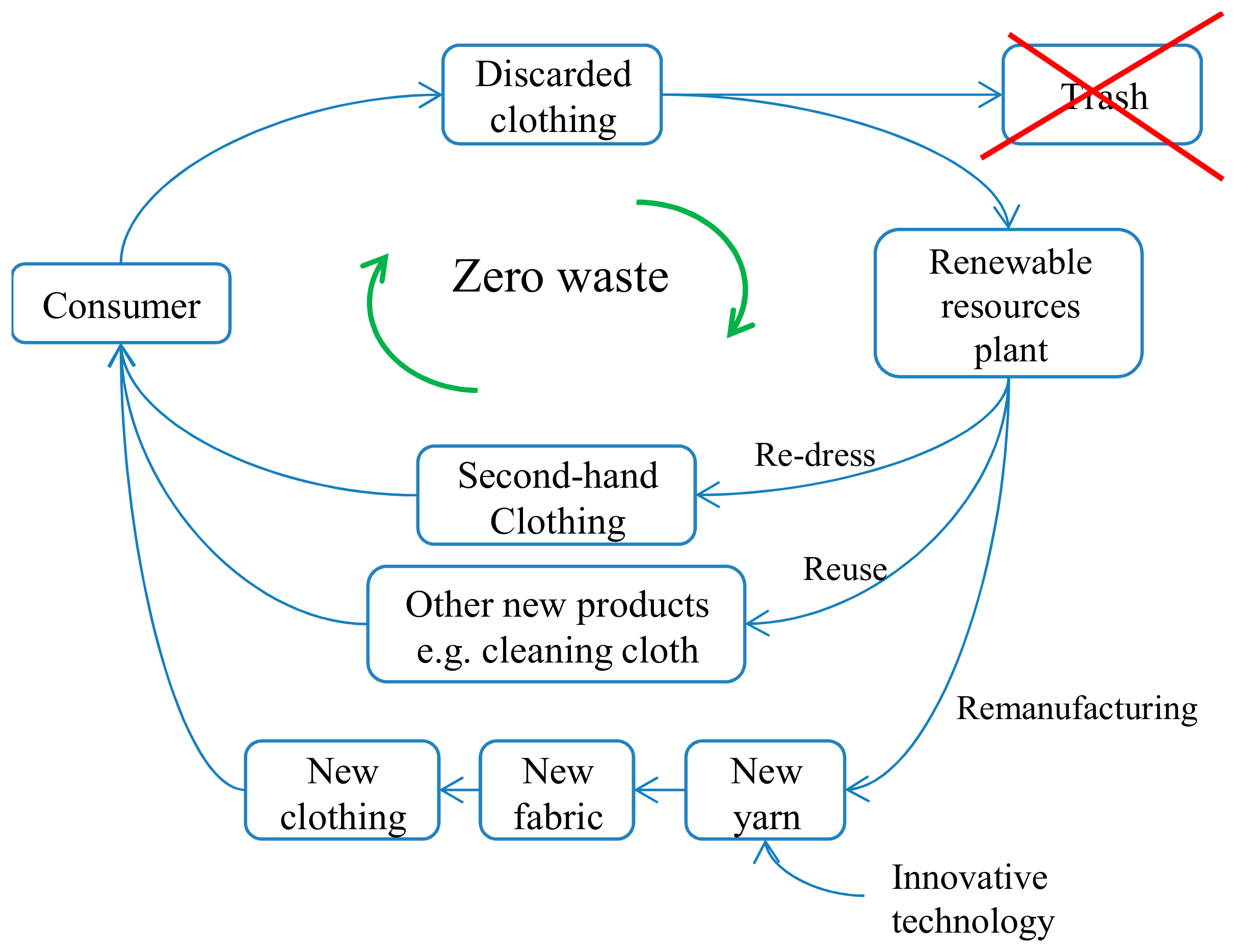
3.1. Case Study: WCRC Selection

With the development of the recycling economy, many recycling and renewable resources companies have emerged in China’s recycling market and the competition has been fierce in the last ten years. Company QL is a waste textile utilization and remanufacturing enterprise in Nanchang, China. The main businesses are waste textile recycling and utilization, clothing, needle textiles, textile raw materials processing and sales. The business of the company focuses on the remanufacturing of waste textiles and the processing and sales of raw materials, while waste clothes are basically purchased from waste recycling points and mobile recyclers. The unstable recycling amount of waste clothes often affects the processing and production of remanufacturing and raw materials. With the increasing pressure of market competition, the company plans to implement a sustainable waste clothing recycling strategy. To this end, the senior managers of company QL plan to implement a large number of layouts in the front-end recycling market and need to increase investment in the most reasonable WCRC. Therefore, the framework proposed in this paper aims to help company QL determine the right WCRC option according to its own requirements.

At present, the waste clothing recycling channels in China mainly include:

(P₁) Franchise point recycling: The company chooses express points, recycling stations and other third parties as franchisees to entrust cooperation recycling.

(P₂) Home recycling: Through the combination of online ordering and offline home recycling, the professional recyclers buy back discarded clothes on time.

(P₃) Recycling boxes: Put waste textile recycling boxes in residential society, colleges and universities, and establish storage and transportation systems.

(P₄) Mail recycling: In the case of fixed unit price, customers place orders online, the express company comes to pick up the pieces, and then the recycling company inspects, weighs and pays for the used clothes.

(P₅) Self-operated store recycling: the company’s own sales agency or site selection in a certain region and self-built waste clothing recycling point.

Through research and market analysis, company QL now invites four DMs {e₁, e₂, e₃, e₄} to provide opinions on WCRC evaluation and selection. These DMs, including a purchasing manager (e₁), a production manager (e₂), a consulting agency director (e₃) and industry association experts (e₄), are competent in decision-making and have nearly ten years of industry experience. The PyFN is expressed for the importance of DMs based on their educational background, knowledge structure, professional level and working time in the industry, and the weight of DMs is calculated according to Equation (10), as shown in

Table 2. DMs’ weights.

DMs	PyFNs	Weights
e1	(0.6,0.5)	0.2043
e2	(0.8,0.3)	0.3036
e3	(0.7,0.6)	0.1996
e4	(0.7,0.3)	0.2925

.

The four DMs evaluated the five WCRC alternatives with regard to six attributes, including recovery size (Y₁), recovery convenience (Y₂), recovery efficiency (Y₃), consumer satisfaction (Y₄), recovery cost (Y₅) and risk bearing (Y₆). All evaluated values are in the form of PyFNs, as shown in

Table 3. Evaluation information of DMs on WCRCs.

DMs	Alternatives	Y1	Y2	Y3	Y4	Y5	Y6
e1	P1	(0.8,0.3)	(0.6,0.5)	(0.5,0.6)	(0.6,0.3)	(0.4,0.7)	(0.6,0.5)
	P2	(0.7,0.4)	(0.8,0.2)	(0.9,0.0)	(0.8,0.3)	(0.8,0.3)	(0.1,0.9)
	P3	(0.9,0.4)	(0.7,0.5)	(0.8,0.2)	(0.7,0.4)	(0.7,0.3)	(0.4,0.6)
	P4	(0.4,0.7)	(0.5,0.7)	(0.9,0.2)	(0.7,0.4)	(0.3,0.8)	(0.9,0.2)
	P5	(0.5,0.6)	(0.5,0.5)	(0.6,0.6)	(0.8,0.5)	(0.6,0.4)	(0.7,0.5)
e2	P1	(0.9,0.0)	(0.7,0.4)	(0.5,0.5)	(0.6,0.5)	(0.4,0.6)	(0.6,0.4)
	P2	(0.8,0.3)	(0.7,0.3)	(0.7,0.4)	(0.7,0.4)	(0.7,0.4)	(0.3,0.8)
	P3	(0.6,0.5)	(0.6,0.4)	(0.7,0.4)	(0.7,0.5)	(0.6,0.5)	(0.5,0.5)
	P4	(0.5,0.8)	(0.4,0.6)	(0.6,0.6)	(0.8,0.3)	(0.2,0.9)	(0.8,0.4)
	P5	(0.7,0.5)	(0.6,0.5)	(0.6,0.3)	(0.7,0.4)	(0.6,0.5)	(0.6,0.5)
e3	P1	(0.8,0.3)	(0.6,0.3)	(0.5,0.6)	(0.8,0.3)	(0.0,0.9)	(0.7,0.5)
	P2	(0.9,0.3)	(0.7,0.4)	(0.8,0.4)	(0.7,0.4)	(0.7,0.5)	(0.5,0.5)
	P3	(0.6,0.6)	(0.7,0.5)	(0.7,0.3)	(0.8,0.0)	(0.4,0.7)	(0.6,0.5)
	P4	(0.4,0.6)	(0.4,0.6)	(0.5,0.5)	(0.5,0.5)	(0.4,0.6)	(0.7,0.3)
	P5	(0.6,0.6)	(0.8,0.5)	(0.6,0.4)	(0.7,0.4)	(0.6,0.6)	(0.6,0.3)
e4	P1	(0.5,0.5)	(0.7,0.4)	(0.5,0.4)	(0.5,0.5)	(0.3,0.8)	(0.4,0.7)
	P2	(0.6,0.5)	(0.8,0.5)	(0.9,0.0)	(0.7,0.4)	(0.7,0.4)	(0.8,0.4)
	P3	(0.7,0.5)	(0.7,0.3)	(0.9,0.3)	(0.8,0.5)	(0.6,0.6)	(0.6,0.5)
	P4	(0.4,0.6)	(0.5,0.5)	(0.9,0.1)	(0.6,0.4)	(0.4,0.6)	(0.8,0.2)
	P5	(0.5,0.5)	(0.6,0.5)	(0.7,0.5)	(0.9,0.2)	(0.5,0.7)	(0.6,0.5)

. Since Y₅ is cost type and other attributes are benefit type, Table 3 is normalized according to Equation (9); the results are presented in

Table 4. Normalized individual PyFDM.

DMs	Alternatives	Y1	Y2	Y3	Y4	Y5	Y6
e1	P1	(0.8,0.3)	(0.6,0.5)	(0.5,0.6)	(0.6,0.3)	(0.7,0.4)	(0.6,0.5)
	P2	(0.7,0.4)	(0.8,0.2)	(0.9,0.0)	(0.8,0.3)	(0.3,0.8)	(0.1,0.9)
	P3	(0.9,0.4)	(0.7,0.5)	(0.8,0.2)	(0.7,0.4)	(0.3,0.7)	(0.4,0.6)
	P4	(0.4,0.7)	(0.5,0.7)	(0.9,0.2)	(0.7,0.4)	(0.8,0.3)	(0.9,0.2)
	P5	(0.5,0.6)	(0.5,0.5)	(0.6,0.6)	(0.8,0.5)	(0.4,0.6)	(0.7,0.5)
e2	P1	(0.9,0.0)	(0.7,0.4)	(0.5,0.5)	(0.6,0.5)	(0.6,0.4)	(0.6,0.4)
	P2	(0.8,0.3)	(0.7,0.3)	(0.7,0.4)	(0.7,0.4)	(0.4,0.7)	(0.3,0.8)
	P3	(0.6,0.5)	(0.6,0.4)	(0.7,0.4)	(0.7,0.5)	(0.5,0.6)	(0.5,0.5)
	P4	(0.5,0.8)	(0.4,0.6)	(0.6,0.6)	(0.8,0.3)	(0.9,0.2)	(0.8,0.4)
	P5	(0.7,0.5)	(0.6,0.5)	(0.6,0.3)	(0.7,0.4)	(0.5,0.6)	(0.6,0.5)
e3	P1	(0.8,0.3)	(0.6,0.3)	(0.5,0.6)	(0.8,0.3)	(0.9,0.0)	(0.7,0.5)
	P2	(0.9,0.3)	(0.7,0.4)	(0.8,0.4)	(0.7,0.4)	(0.5,0.7)	(0.5,0.5)
	P3	(0.6,0.6)	(0.7,0.5)	(0.7,0.3)	(0.8,0.0)	(0.7,0.4)	(0.6,0.5)
	P4	(0.4,0.6)	(0.4,0.6)	(0.5,0.5)	(0.5,0.5)	(0.6,0.4)	(0.7,0.3)
	P5	(0.6,0.6)	(0.8,0.5)	(0.6,0.4)	(0.7,0.4)	(0.6,0.6)	(0.6,0.3)
e4	P1	(0.5,0.5)	(0.7,0.4)	(0.5,0.4)	(0.5,0.5)	(0.8,0.3)	(0.4,0.7)
	P2	(0.6,0.5)	(0.8,0.5)	(0.9,0.0)	(0.7,0.4)	(0.4,0.7)	(0.8,0.4)
	P3	(0.7,0.5)	(0.7,0.3)	(0.9,0.3)	(0.8,0.5)	(0.6,0.6)	(0.6,0.5)
	P4	(0.4,0.6)	(0.5,0.5)	(0.9,0.1)	(0.6,0.4)	(0.6,04)	(0.8,0.2)
	P5	(0.5,0.5)	(0.6,0.5)	(0.7,0.5)	(0.9,0.2)	(0.7,0.5)	(0.6,0.5)

. The evaluation information of the four DMs is aggregated by Equation (11) to generate the aggregated PyFDM, as shown in

Table 5. The aggregated PyFDM of WCRCs.

Alternatives	Y1	Y2	Y3	Y4	Y5	Y6
P1	(0.947,0.070)	(0.864,0.142)	(0.707,0.241)	(0.838,0.153)	(0.935,0.078)	(0.790,0.255)
P2	(0.936,0.119)	(0.927,0.162)	(0.969,0.062)	(0.908,0.117)	(0.596,0.467)	(0.770,0.382)
P3	(0.909,0.244)	(0.871,0.164)	(0.952,0.097)	(0.927,0.182)	(0.766,0.292)	(0.748,0.229)
P4	(0.630,0.488)	(0.654,0.324)	(0.949,0.109)	(0.879,0.122)	(0.939,0.075)	(0.957,0.079)
P5	(0.803,0.257)	(0.844,0.239)	(0.838,0.204)	(0.952,0.125)	(0.788,0.279)	(0.830,0.196)

.

Based on the PyF-ITARA approach in Step 3.1, PyFDM H is constructed, and its calculation process based on Equation (12) is shown in Figure 2. Then, the attribute objective weight vector w^o = (0.165,0.161,0.179,0.188,0.150,0.158)^T is calculated by Equations (13) and (14). DMs give evaluation information in the form of PyFN for the importance of related attributes, and we utilize Equations (15)–(17) to calculate the subjective weight of attributes. The results are listed in

Table 6. The subjective weights of attributes.

Attributes	e1	e2	e3	e4	ωj	sc(ωj)	wjs
Y1	(0.5,0.4)	(0.7,0.5)	(0.4,0.6)	(0.3,0.7)	(0.734,0.283)	0.729	0.148
Y2	(0.7,0.4)	(0.8,0.2)	(0.9,0.3)	(0.7,0.4)	(0.945,0.098)	0.942	0.192
Y3	(0.8,0.5)	(0.5,0.6)	(0.6,0.5)	(0.5,0.7)	(0.818,0.314)	0.785	0.160
Y4	(0.5,0.5)	(0.6,0.4)	(0.7,0.4)	(0.8,0.3)	(0.877,0.123)	0.877	0.179
Y5	(0.9,0.1)	(0.7,0.4)	(0.9,0.2)	(0.7,0.4)	(0.955,0.072)	0.954	0.194
Y6	(0.4,0.6)	(0.4,0.6)	(0.6,0.4)	(0.3,0.8)	(0.625,0.372)	0.626	0.127

.

Thus, the combined weight vector of attributes can be calculated according to Equation (17), w^c = (0.147,0.185,0.172,0.201,0.175,0.120)^T.

We construct an extended PyFDM based on Table 5, as shown in

Table 7. The extended PyFDM of WCRCs.

Alternatives	Y1	Y2	Y3	Y4	Y5	Y6
NIS	(0630,0.488)	(0654,0.324)	(0707,0.241)	(0.838,0.182)	(0.596,0.467)	(0.748,0.382)
P1	(0.947,0.070)	(0.864,0.142)	(0.707,0.241)	(0.838,0.153)	(0.935,0.078)	(0.790,0.255)
P2	(0.936,0.119)	(0.927,0.162)	(0.969,0.062)	(0.908,0.117)	(0.596,0.467)	(0.770,0.382)
P3	(0.909,0.244)	(0.871,0.164)	(0.952,0.097)	(0.927,0.182)	(0.766,0.292)	(0.748,0.229)
P4	(0.630,0.488)	(0.654,0.324)	(0.949,0.109)	(0.879,0.122)	(0.939,0.075)	(0.957,0.079)
P5	(0.803,0.257)	(0.844,0.239)	(0.838,0.204)	(0.952,0.125)	(0.788,0.279)	(0.830,0.196)
PIS	(0.947,0.070)	(0.927,0.142)	(0.969,0.062)	(0.952,0.117)	(0.939,0.076)	(0.957,0.079)

. We apply the PyF-CoCoSo-D method (Equations (19)–(23)) to calculate the comprehensive utility values of all alternatives (φ = 0.5), as shown in

Table 8. The aggregation strategies and final sorting result of WCRCs.

Alternatives	${\mathit{\wp }}^{(1)}$	${\mathit{\wp }}^{(2)}$	${\partial }_{\mathit{i}}^{(1)}$	${\partial }_{\mathit{i}}^{(2)}$	Kia	Kib	Kic	Ki	Ranking
NIS	(0.901,0.104)	(0.898,0.123)	-	-	-	-	-	-	-
P1	(0.980,0.018)	(0.979,0.029)	0.813	0.815	0.194	2.066	0.918	1.776	4
P2	(0.988,0.031)	(0.985,0.087)	0.902	0.869	0.211	2.248	0.999	1.932	1
P3	(0.985,0.034)	(0.985,0.040)	0.871	0.872	0.207	2.211	0.982	1.900	2
P4	(0.984,0.031)	(0.980,0.085)	0.856	0.826	0.200	2.134	0.948	1.834	3
P5	(0.977,0.035)	(0.977,0.043)	0.787	0.789	0.188	2.000	0.888	1.719	5
PIS	(0.997,0.008)	(0.997,0.009)	-	-	-	-	-	-	-

. According to the comprehensive utility value K_i, the WCRCs are finally ranked as P₂ > P₃ > P₄ > P₁ > P₅. Therefore, P₂ (Home recycling) is the best option.

The results show that Home recycling performs best in the attributes in this study, followed by Recycling boxes. The other three alternatives are significantly different from these two. This means that company QL needs to increase investment in the recycling channel of waste clothing for Home recycling. The weight vector w^c = (0.147,0.185,0.172,0.201,0.175,0.120)^T. We can see how the attribute ranking, namely consumer satisfaction (Y₄) > recovery convenience (Y₂) > recovery cost (Y₅) > recovery efficiency (Y₃) > recovery size (Y₁) > risk bearing (Y₆). The company QL also needs to focus on consumer satisfaction and recovery convenience.

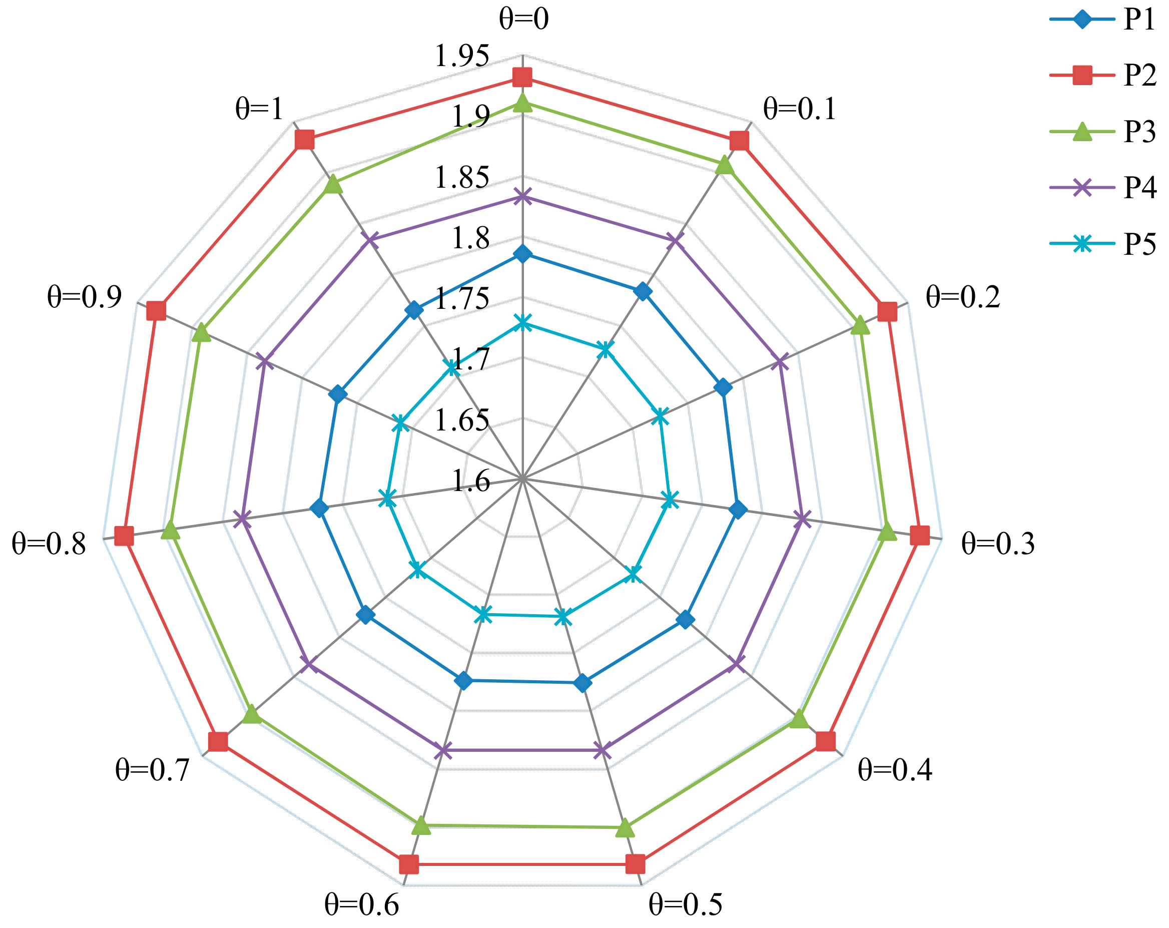
3.2. Sensitivity Analysis

This sub-section further analyzes the influence of parameter θ variation on the compromise ranking result of the proposed method. Let the parameter θ within the range of [0,1] for the experiment.

Table 9. The change of comprehensive utility value of alternatives with different θ.

Alternatives	θ = 0.0	θ = 0.1	θ = 0.2	θ = 0.3	θ = 0.4	θ = 0.5	θ = 0.6	θ = 0.7	θ = 0.8	θ = 0.9	θ = 0.9
P1	1.786	1.784	1.782	1.780	1.778	1.776	1.774	1.772	1.770	1.768	1.766
P2	1.931	1.931	1.932	1.932	1.932	1.932	1.932	1.932	1.933	1.933	1.933
P3	1.911	1.909	1.906	1.904	1.902	1.900	1.898	1.896	1.894	1.892	1.890
P4	1.833	1.833	1.833	1.834	1.834	1.834	1.834	1.834	1.834	1.834	1.834
P5	1.729	1.727	1.725	1.723	1.721	1.719	1.717	1.715	1.713	1.711	1.709

and Figure 3 present the numerical results and the alternative ordering results, respectively. From them, we find that the score values of P₁, P₃ and P₅ decrease slightly from the overall perspective, while P₂ and P₄ increase slightly. Nevertheless, the ranking of alternatives is still P₂ > P₃ > P₄ > P₁ > P₅. Therefore, the different values of parameter θ do not change the alternatives’ ranking order, which indicates that the proposed method has sufficient stability at different θ values. It is not difficult to find that the best option is P₂, and P₅ is the worst. We can conclude that our method is not affected by any bias and the results are stable and feasible in nature.

Next, we examine the influence on the alternative ranking by changing attribute weights. For this purpose, we adopt 8 scenarios, among which the attribute weight vector of this paper is used in scenario #0. In scenario #1, the attribute weight values are assumed to be equal. In scenarios #2~#7, it is assumed that the weight value of one attribute is 0.5 and the weight values of the other attributes are 0.1. Thus, we obtain the ranking results of alternatives, as shown in

Table 10. The ranking results of different scenarios.

Scenarios	Y1	Y2	Y3	Y4	Y5	Y6	Ranking
#0	w1 = 0.147	w2 = 0.185	w3 = 0.172	w4 = 0.201	w5 = 0.175	w6 = 0.120	P2 > P3 > P4 > P1 > P5
#1	w1 = 0.167	w2 = 0.167	w3 = 0.167	w4 = 0.167	w5 = 0.167	w6 = 0.167	P2 > P3 > P4 > P1 > P5
#2	w1 = 0.500	w2 = 0.100	w3 = 0.100	w4 = 0.100	w5 = 0.100	w6 = 0.100	P2 > P1 > P3 > P5 > P4
#3	w1 = 0.100	w2 = 0.500	w3 = 0.100	w4 = 0.100	w5 = 0.100	w6 = 0.100	P2 > P3 > P1 > P5 > P4
#4	w1 = 0.100	w2 = 0.100	w3 = 0.500	w4 = 0.100	w5 = 0.100	w6 = 0.100	P2 > P3 > P4 > P5 > P51
#5	w1 = 0.100	w2 = 0.100	w3 = 0.100	w4 = 0.500	w5 = 0.100	w6 = 0.100	P5 > P3 > P2 > P4 > P1
#6	w1 = 0.100	w2 = 0.100	w3 = 0.100	w4 = 0.100	w5 = 0.500	w6 = 0.100	P4 > P1 > P3 > P5 > P4
#7	w1 = 0.100	w2 = 0.100	w3 = 0.100	w4 = 0.100	w5 = 0.100	w6 = 0.500	P4 > P2 > P5 > P1 > P3

. The alternative ranking changes in different scenarios, as shown in Figure 4.

From Table 10 and Figure 4, in scenarios #0~#4, when the maximum weight attribute changes from Y₁ to Y₃, the optimal alternative is still P₂, but the ranking of the other alternatives has changed. In scenarios #5~7, the best alternative P₅ and P₄ in the process of changing the maximum weight attribute are from Y₄ to Y₆, respectively. This shows that the change in attribute weight can affect the alternative ranking result.

3.3. Comparison with Existing Methods

In this subsection, a comparative study is carried out using weighting methods and sorting methods to illustrate the effectiveness and superiority of the proposed method.

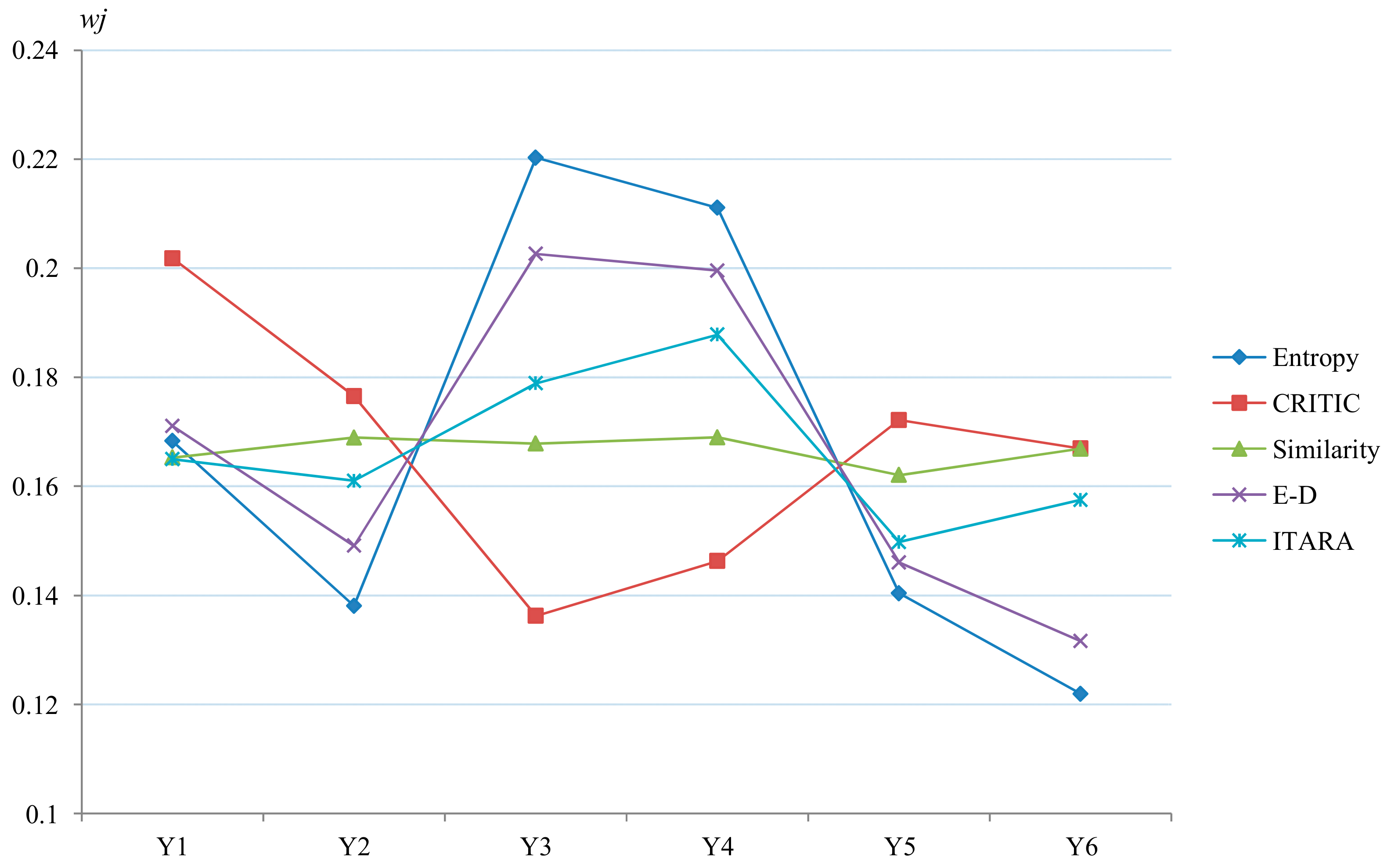
3.3.1. Comparison of Weighting Methods

In the Pythagorean fuzzy environment, we choose the Entropy weighting method [20], CRITIC method [66], Similarity measure [78], and Entropy-Deviation (E-D) method [36] to compare with the PyF-ITARA method. We calculate the data in the aggregated PyFDM by the above four weighting methods to compute the attribute objective weights. The results calculated by weighting methods are listed in

Table 11. The objective weights of attributes calculated by different weighting approaches.

Weighting Approaches	Y1	Y2	Y3	Y4	Y5	Y6
Entropy [20]	0.168	0.138	0.220	0.211	0.140	0.122
CRITIC [66]	0.202	0.177	0.136	0.146	0.172	0.167
Similarity [78]	0.165	0.169	0.168	0.169	0.162	0.167
E-D [36]	0.171	0.149	0.203	0.200	0.146	0.132
ITARA	0.165	0.161	0.179	0.188	0.150	0.158

, and Figure 5 shows a comparison of the weighting methods.

As can be seen from Table 11 and Figure 5, the order of weight of each attribute calculated by the PyF-ITARA method is completely different from the results of the CRITIC and Similarity measure. This is similar to the overall distribution of attribute weights for the Entropy and E-D methods. The Entropy and E-D methods obtain the maximum weight value for attribute Y₃ and the minimum weight value for attribute Y₆, but the PyF-ITARA method in this paper obtains the maximum weight value for attribute Y₄ and the minimum weight value for attribute Y₅. In terms of the importance distribution of attribute weight, the PyF-ITARA method does not overemphasize the importance of Y₄ or the unimportance of Y₅, which is more consistent with the actual decision-making. In the calculation process, the existing methods all prematurely de-fuzzize the evaluation information, while the PyF-ITARA method in this paper uses MD and ND separately and in parallel. Meanwhile, the PyF-ITARA method has less computation and more applicability and operability in determining the weight of attributes compared with these methods.

3.3.2. Compared with Existing Sorting Methods

Existing Pythagorean fuzzy MADM techniques, such as PyF-TOPSIS [79], PyF-VIKOR [36], PyF-WASPAS [83], PyF-MULTIMOORA [84] and PyF-CoCoSo [78], are used to calculate the case in this paper to verify the effectiveness of our method. The calculations are listed in

Table 12. The results of different methods.

Alternatives	CoCoSo-D	TOPSIS [79]	WASPAS [83]	MULTIMOORA [84]	CoCoSo [78]	VIKOR [36]
P1	Q1 = 1.776	ξ1 = 0.507	sc(Q1) = 0.715	U1 = 0.936	Q1 = 1.907	Q1 = 1.000
P2	Q2 = 1.932	ξ2 = 0.591	sc(Q2) = 0.739	U2 = 1.000	Q2 = 1.923	Q2 = 0.202
P3	Q3 = 1.900	ξ3 = 0.570	sc(Q3) = 0.732	U3 = 0.952	Q3 = 1.938	Q3 = 0.355
P4	Q4 = 1.834	ξ4 = 0.516	sc(Q4) = 0.624	U4 = 0.815	Q4 = 1.759	Q4 = 0.545
P5	Q5 = 1.719	ξ5 = 0.462	sc(Q5) = 0.603	U5 = 0.780	Q5 = 1.703	Q5 = 0.230
Ranking	P2 > P3 > P4 > P1 > P5	P2 > P3 > P4 > P1 > P5	P2 > P3 > P1 > P4 > P5	P2 > P3 > P1 > P4 > P5	P3 > P2 > P1 > P4 > P5	P2 > P3 > P5 > P4 > P1
Spearman’s correlation	-	1	0.9	0.9	0.8	0.7

.

From Table 12, TOPSIS [79] used the idea of approaching the ideal solution to obtain the relative closeness values. The ranking of alternatives is consistent with the method proposed, and the best option is P₂. The final ranking obtained by WASPAS [83] is slightly different from that obtained in this paper. In WASPAS [83], the PyFWA and PyFWG operators are used to aggregate the evaluation values of each attribute. Similarly, MULTIMOORA [84] also uses the PyFWA and PyFWG operators to calculate the ratio system model and full multiplicative form of each alternative. CoCoSo [78] also obtains the WSM and WPM models of the alternative through the PyFWA and PyFWG operators, and then calculates the three strategies and obtains the equilibrium compromise solution of the alternative, but P₃ is the best option. The VIKOR [36] method adopts a divergence measure with an ideal solution and compromises between individual regret and group utility to obtain the final ordering. P₂ is the best option, but the ranking of others differs from the method proposed. To sum up, alternative P₂ has the most important value of all options. This also shows the effectiveness and feasibility of the proposed method.

The PyFWA and PyFWG operators can be found in WASPAS [83], MULTIMOORA [84] and CoCoSo [78] methods. These AOs are mainly based on basic AOLs, and the score function is utilized to defuzzify the results of these AOs. As a result, the interaction between membership functions in PyFNs is not shown in the process of evaluation information fusion, and the preference of DMs on evaluation objects is not reflected in the decision results. In addition, premature precision makes part of the evaluation information lost. Because the CoCoSo-D method in this paper applies the STI-PyFWA and STI-PyFWG operators based on the STIOLs and distance measure to determine the final alternatives sorting, these are essentially different from the existing methods. Thus, the characteristics of the above methods are compared in

Table 13. Comparison with different methods.

Characteristics	This Paper	Zhang and Xu [79]	Rani et al. [83]	Sarkar and Biswas [84]	Liu et al. [78]	Rani et al. [36]
Approaches	CoCoSo-D	TOPSIS	WASPAS	MULTIMOORA	CoCoSo	VIKOR
Decision type	Group	Single	Group	Group	Group	Group
Experts’ weights	Computed	Not Applicable	Computed	Assumed	Computed	Computed
Criteria weights	Combined	Assumed	Combined	Objective	Combined	Combined
Weighting methods	Subjective evaluation/ITARA	-	Subjective evaluation/E-D	Entropy	Subjective evaluation/similarity measure	Subjective evaluation/E-D
OLs	STIOLs	AOLs	AOLs	AOLs	AOLs	AOLs
AOs	STI-PyFWA, STI-PyFWG	PyFWA	PyFWA, PyFWG	PyFWA, PyFWG	PyFWA, PyFWG	PyFWA
Defuzzification techniques	Distance measure	Distance measure	Score function	Score function/Distance measure	Score function	Divergence measure
Decision mechanism	Compromise	Similarity to ideal solution	Score function	WSM	Compromise	Compromise

.

Furthermore, the three main advantages of this method are summarized based on the above comparison.

(1) In the Pythagorean fuzzy MAGDM problem, except for the Entropy weighting model in Sarkar and Biswas [84] to calculate the objective weight of attributes, other group decision-making methods adopt the combination weight of subjective and objective. Among these combined weights, Rani et al. [36,83] calculate the objective weight of attributes based on the E-D technique. Liu et al. [78] uses the Similarity measure to obtain the objective weight of an attribute. In this article, the ITARA approach is extended and applied to obtain the semi-objective weight of the attribute in the Pythagorean fuzzy environment. The calculation process of the PyF-ITARA method is simple to compare with the existing methods for calculating the objective weight of the attribute.

(2) In the process of PyFN aggregation and fusion, the selection of operation rules is a vital step. However, the PyFWA or PyFWG operators cannot deal well with MD or ND being zero problems. Therefore, we combine STOLs with IOLs to develop STIOLs, the STI-PyFWA and STI-PyFWG operators, which can not only retain the periodicity and symmetry of origin to satisfy DMs’ preference for multi-time phase parameters, but also eliminate the counterintuitive phenomenon caused by MD or ND being zero. Furthermore, the STI-PyFWA and STI-PyFWG operators replace WSM and WPM in traditional CoCoSo methods.

(3) In the PyF-CoCoSo method [78], the values of WSM and WPM models are de-fuzzified by score function [17] when calculating the three aggregation strategies of the alternatives. The distance measure with hesitation [80] is a feasible way to determine the difference, which can distinguish two PyFNs more effectively than the score function. Therefore, we use the distance measure between the alternative and the ideal solution to take over the score function in the PyF-CoCoSo-D method. Although the calculation process is relatively complex, the final ranking result of the alternative is more accurate and reasonable. Meanwhile, the calculation process of the proposed method is relatively simple to compare with the compromise solution of VIKOR [36].

4. Conclusions

The WCRC selection under circular economy is regarded as a typical MAGDM problem, the STIOLs are first defined in Pythagorean fuzzy environment, the STI-PyFWA and STI-PyFWG operators are proposed based on this, and some related desirable properties are discussed. Then, we propose the PyFMAGDM framework based on the CoCoSo-D method. The subjective weight of attributes is determined by the DMs’ subjective evaluation, the objective weight is calculated by the improved PyF-ITARA approach, and the combined weight of attributes is obtained. The traditional CoCoSo method is modified by the AOs and Pythagorean fuzzy distance measure. The optimal WCRC is obtained by applying the proposed method in the case study. The sensitivity analysis and comparison study are implemented to verify the effectiveness and superiority. However, there are still three limitations of the proposed method in this paper:

• The process of determining the weight of DMs in this paper is simple and subjective, without considering the correlation of DMs’ preferences.
• This paper does not take into account the interrelationship between attribute variables in the process of attribute weight determination and information aggregation.
• Although the proposed method contains one parameter, its flexibility is limited, and the proposed method cannot better and flexibly express the preferences and attitudes of DMs in information fusion.

In the future, we will extend the proposed STIOLs to other fuzzy theories, such as spherical FS (SFS) [85] and T-spherical FS (TSFS) [86,87], interval valued TSFS (IVTSFS) [88], etc. We will try to carry out integration studies with BM, MSM, HM and CI operators that can capture the interrelationship of attribute variables. Meanwhile, we will combine this with other relatively new decision-making techniques (e.g., WASPAS, MARCOS, etc.), and they will be utilized in a wider range of fields in real life.

References

1. Holmes, L. New Lifestyles System Data: 2016 Global Consumer Trends Survey Results. 2016. Available online: https://blog.euromonitor.com/new-lifestyles-system-data-2016-global-consumer-trends-survey-results/ (accessed on 11 October 2020).
2. Leal Filho, W.; Ellams, D.; Han, S.; Tyler, D.; Boiten, V.J.; Paco, A.; Moora, H.; Balogun, A.L. A review of the socio-economic advantages of textile recycling. J. Clean. Prod. 2019, 218, 10–20. [Google Scholar] [CrossRef]
3. Kerr, J.; Landry, J. Pulse of the Fashion Industry; Global Fashion Agenda: Copenhagen, Sweden, 2017. [Google Scholar]
4. United Nations Environment Programme. Putting the Brakes on Fast Fashion. 2018. Available online: https://www.unenvironment.org./news-and-stories/story/putting-brakes-fast-fashion (accessed on 12 November 2018).
5. Panwar, R.; Niesten, E. Advancing circular economy. Bus. Strategy Environ. 2020, 29, 2890–2892. [Google Scholar] [CrossRef]
6. Brismar, A. Circular Fashion. 2019. Available online: https://circularfashion.com/circular-fashion-definition/ (accessed on 30 September 2019).
7. Kaisa, V.; Anne, R.; Pirjo, H.; Ali, H. Consumer attitudes and communication in circular fashion. J. Fash. Mark. Manag. 2018, 22, 286–300. [Google Scholar]
8. Ki, C.W.; Chong, S.M.; Ha-Brookshire, J.E. How fashion can achieve sustainable development through a circular economy and stakeholder engagement: A systematic literature review. Corp. Soc. Responsib. Environ. Manag. 2020, 27, 2401–2424. [Google Scholar] [CrossRef]
9. Ki, C.W.; Park, S.; Ha-Brookshire, J.E. Toward a circular economy: Understanding consumers’ moral stance on corporations’ and individuals’ responsibilities in creating a circular fashion economy. Bus. Strategy Environ. 2021, 30, 1121–1135. [Google Scholar] [CrossRef]
10. Lin, C.W.R.; Chen, M.T.; Tseng, M.L.; Jantarakolica, T.; Xu, H. Multi-objective production programming to systematic sorting and remanufacturing in second-hand clothing recycling industry. Symmetry 2020, 12, 1161. [Google Scholar] [CrossRef]
11. Mi, S. Unspoken Crisis: Mounting Textile Waste in China. 2018. Available online: http://www.coresponsibility.com/unspoken-crisis-mounting-textile-waste-in-china/ (accessed on 5 July 2018).
12. Zhang, L.; Wu, T.; Liu, S.; Jiang, S.Y.; Wu, H.J.; Yang, J.M. Consumers’ clothing disposal behaviors in Nanjing, China. J. Clean. Prod. 2020, 276, 123184. [Google Scholar] [CrossRef]
13. Zadeh, L.A. Fuzzy sets. Inf. Control 1965, 8, 338–353. [Google Scholar] [CrossRef] [Green Version]
14. Atanassov, K. Intuitionistic fuzzy sets. Fuzzy Sets Syst. 1986, 31, 343–349. [Google Scholar] [CrossRef]
15. Yager, R.R. Pythagorean membership grades in multicriteria decision making. IEEE Trans. Fuzzy Syst. 2014, 22, 958–965. [Google Scholar] [CrossRef]
16. Wei, G.W. Pythagorean fuzzy interaction aggregation operators and their application to multiple attribute decision making. J. Intell. Fuzzy Syst. 2017, 33, 2119–2132. [Google Scholar] [CrossRef]
17. Wei, G.W.; Lu, M. Pythagorean fuzzy power aggregation operators in multiple attribute decision making. Int. J. Intell. Syst. 2018, 33, 169–186. [Google Scholar] [CrossRef]
18. Gao, H. Pythagorean fuzzy Hamacher Prioritized aggregation operators in multiple attribute decision making. J. Intell. Fuzzy Syst. 2018, 35, 2229–2245. [Google Scholar] [CrossRef]
19. Wang, L.; Li, N. Pythagorean fuzzy interaction power Bonferroni mean aggregation operators in multiple attribute decision making. Int. J. Intell. Syst. 2020, 35, 150–183. [Google Scholar] [CrossRef]
20. Wang, L.; Garg, H.; Li, N. Pythagorean fuzzy interactive Hamacher power aggregation operators for assessment of express service quality with entropy weight. Soft Comput. 2020, 25, 973–993. [Google Scholar] [CrossRef]
21. Wei, G.W. Pythagorean fuzzy Maclaurin symmetric mean operators in multiple attribute decision making. Int. J. Intell. Syst. 2018, 33, 1043–1070. [Google Scholar] [CrossRef]
22. Chen, T.Y. Remoteness index-based Pythagorean fuzzy VIKOR methods with a generalized distance measure for multiple criteria decision analysis. Inf. Fusion 2018, 41, 129–150. [Google Scholar] [CrossRef]
23. Akram, M.; Ilyas, F.; Garg, H. Multi-criteria group decision making based on ELECTRE I method in Pythagorean fuzzy information. Soft Comput. 2020, 24, 3425–3453. [Google Scholar] [CrossRef]
24. Ren, P.J.; Xu, Z.S.; Gou, X.J. Pythagorean fuzzy TODIM approach to multi-criteria decision making. Appl. Soft Comput. 2016, 42, 246–259. [Google Scholar] [CrossRef]
25. Gul, M.; Ak, M.F.; Guneri, A.F. Pythagorean fuzzy VIKOR-based approach for safety risk assessment in mine industry. J. Safety Res. 2019, 69, 135–153. [Google Scholar] [CrossRef]
26. Peng, X.D.; Yang, Y. Pythagorean fuzzy Choquet integral based MABAC method for multiple attribute Ggroup Ddecision Mmaking. Int. J. Intell. Syst. 2016, 31, 989–1020. [Google Scholar] [CrossRef]
27. Akram, M.; Luqman, A.; Alcantud, J.C.R. Risk evaluation in failure modes and effects analysis: Hybrid TOPSIS and ELECTRE I solutions with Pythagorean fuzzy information. Neural Comput. Appl. 2021, 33, 5675–5703. [Google Scholar] [CrossRef]
28. Peng, X.D.; Ma, X.L. Pythagorean fuzzy multi-criteria decision making method based on CODAS with new score function. J. Intell. Fuzzy Syst. 2020, 38, 3307–3318. [Google Scholar] [CrossRef]
29. Li, P.; Liu, J.; Wei, C.P.; Liu, J. A new EDAS method based on prospect theory for Pythagorean fuzzy set and its application in selecting investment projects for highway. Kybernetes 2021, in press. [Google Scholar] [CrossRef]
30. Huang, C.; Lin, M.W.; Xu, Z.S. Pythagorean fuzzy MULTIMOORA method based on distance measure and score function: Its application in multicriteria decision making process. Knowl. Inf. Syst. 2020, 62, 4373–4406. [Google Scholar] [CrossRef]
31. Zhang, Z.X.; Hao, W.N.; Yu, X.H.; Chen, G.; Zhang, S.J.; Chen, J.Y. Pythagorean fuzzy preference ranking organization method of enrichment evaluations. Int. J. Intell. Syst. 2019, 34, 1416–1439. [Google Scholar] [CrossRef]
32. Molla, M.U.; Giri, B.C.; Biswas, P. Extended PROMETHEE method with Pythagorean fuzzy sets for medical diagnosis problems. Soft Comput. 2021, 25, 4503–4512. [Google Scholar] [CrossRef]
33. Zhao, M.W.; Wei, G.W.; Wei, C.; Wu, J. Pythagorean fuzzy TODIM method based on the cumulative prospect theory for MAGDM and its application on risk assessment of science and technology projects. Int. J. Fuzzy Syst. 2021, 23, 1027–1041. [Google Scholar] [CrossRef]
34. Akram, M.; Dudek, W.A.; Ilyas, F. Group decision-making based on Pythagorean fuzzy TOPSIS method. Int. J. Intell. Syst. 2019, 34, 1455–1475. [Google Scholar] [CrossRef]
35. Sarkar, B.; Biswas, A. Pythagorean fuzzy AHP-TOPSIS integrated approach for transportation management through a new distance measure. Soft Comput. 2021, 25, 4073–4089. [Google Scholar] [CrossRef]
36. Rani, P.; Mishra, A.R.; Pardasani, K.R.; Mardani, A.; Liao, H.C.; Streimikiene, D. A novel VIKOR approach based on entropy and divergence measures of Pythagorean fuzzy sets to evaluate renewable energy technologies in India. J. Clean. Prod. 2019, 238, 117936. [Google Scholar] [CrossRef]
37. Alrasheedi, M.; Mardani, A.; Mishra, A.R.; Rani, P.; Loganathan, N. An extended framework to evaluate sustainable suppliers in manufacturing companies using a new Pythagorean fuzzy entropy-SWARA-WASPAS decision-making approach. J. Enterp. Inf. Manag. 2021, in press. [Google Scholar] [CrossRef]
38. Ayyildiz, E.; Erdogan, M.; Gumus, A.T. A Pythagorean fuzzy number-based integration of AHP and WASPAS methods for refugee camp location selection problem: A real case study for Istanbul, Turkey. Neural Comput. Appl. 2021, 33, 15751–15768. [Google Scholar] [CrossRef]
39. Garg, H. New exponential operational laws and their aggregation operators for interval-valued Pythagorean fuzzy multicriteria decision-making. Int. J. Intell. Syst. 2018, 33, 653–683. [Google Scholar] [CrossRef]
40. Garg, H. New logarithmic operational laws and their aggregation operators for Pythagorean fuzzy set and their applications. Int. J. Intell. Syst. 2019, 34, 82–106. [Google Scholar] [CrossRef] [Green Version]
41. Ashraf, S.; Abdullah, S. Decision aid modeling based on sine trigonometric spherical fuzzy aggregation information. Soft Compu. 2021, 25, 8549–8572. [Google Scholar] [CrossRef]
42. Garg, H. Sine trigonometric operational laws and its based Pythagorean fuzzy aggregation operators for group decision-making process. Artif. Intell. Rev. 2021, 54, 4421–4447. [Google Scholar] [CrossRef]
43. Ashraf, S.; Abdullah, S.; Khan, S. Fuzzy decision support modeling for internet finance soft power evaluation based on sine trigonometric Pythagorean fuzzy information. J. Ambient. Intell. Humaniz. Comput. 2021, 12, 3101–3119. [Google Scholar] [CrossRef]
44. Ashraf, S.; Abdullah, S.; Zeng, S.; Jin, H.; Ghanin, F. Fuzzy decision support modeling for hydrogen power plant selection based on single value neutrosophic sine trigonometric aggregation operators. Symmetry 2020, 12, 298. [Google Scholar] [CrossRef] [Green Version]
45. Garg, H. A novel trigonometric operation-based q-rung orthopair fuzzy aggregation operator and its fundamental properties. Neural Comput. Appl. 2020, 32, 15077–15099. [Google Scholar] [CrossRef]
46. He, Y.D.; Chen, H.Y.; Zhou, L.G.; Liu, J.P.; Tao, Z.F. Intuitionistic fuzzy geometric interaction averaging operators and their application to multi-criteria decision making. Inf. Sci. 2014, 259, 142–159. [Google Scholar] [CrossRef]
47. Lin, M.W.; Li, X.M.; Chen, L.F. Linguistic q-rung orthopair fuzzy sets and their interactional partitioned Heronian mean aggregation operators. Int. J. Intell. Syst. 2020, 35, 217–249. [Google Scholar] [CrossRef]
48. Yang, Z.L.; Garg, H. Interaction power partitioned Maclaurin Symmetric mean operators under q-rung orthopair uncertain linguistic information. Int. J. Fuzzy Syst. 2021, 1–19. (in press). [Google Scholar] [CrossRef]
49. Garg, H.; Arora, R. Novel scaled prioritized intuitionistic fuzzy soft interaction averaging aggregation operators and their application to multi criteria decision making. Eng. Appl. Artif. Intell. 2018, 71, 100–112. [Google Scholar] [CrossRef]
50. Garg, H. Generalized intuitionistic fuzzy interactive geometric aggregation operators using Einstein t-norm and t-conorm and their application to decision making. Comput. Ind. Eng. 2016, 101, 53–69. [Google Scholar] [CrossRef]
51. Liu, P.D.; Chen, S.M.; Liu, J.L. Multiple attribute group decision making based on intuitionistic fuzzy interaction partitioned Bonfereoni mean operators. Inf. Sci. 2017, 411, 98–121. [Google Scholar] [CrossRef]
52. Hatefi, M.A. Indifference threshold-based attribute ratio analysis: A method for assigning the weights to the attributes in multiple attribute decision making. Appl. Soft Comput. 2019, 74, 643–651. [Google Scholar] [CrossRef]
53. Liu, P.D.; Pan, Q.; Xu, H.X. Multi-attribute border approximation area comparison (MABAC) method based on normal q-rung orthopair fuzzy environment. J. Intell. Fuzzy Syst. 2021, 40, 9085–9111. [Google Scholar] [CrossRef]
54. Chang, T.W.; Pai, C.J.; Lo, H.W.; Hu, S.K. A hybrid decision-making model for sustainable supplier evaluation in electronics manufacturing. Comp. Ind. Eng. 2021, 156, 107283. [Google Scholar] [CrossRef]
55. Alper Sofuoğlu, M. Development of an ITARA-based hybrid multi-criteria decision-making model for material selection. Soft Comput. 2019, 23, 6715–6725. [Google Scholar] [CrossRef]
56. Du, P.L.; Chen, Z.; Gong, X.M. Load response potential evaluation for distribution networks: A hybrid decision-making model with intuitionistic normal cloud and unknown weight information. Energy 2020, 192, 116673. [Google Scholar] [CrossRef]
57. Gong, J.W.; Li, Q.; Yin, L.S.; Liu, H.C. Undergraduate teaching audit and evaluation using an extended MABAC method under q-rung orthopair fuzzy environment. Int. J. Intell. Syst. 2020, 35, 1912–1933. [Google Scholar] [CrossRef]
58. Ulutas, A.; Karabasevic, D.; Popovic, G.; Stanujkic, D.; Nguyen, P.T.; Karakoy, C. Development of a novel integrated CCSD-ITARA-MARCOS decision-making approach for stackers selection in a logistics system. Mathematics 2020, 8, 1672. [Google Scholar] [CrossRef]
59. Lo, H.W.; Hsu, C.C.; Huang, C.N.; Liou, J.J.H. An ITARA-TOPSIS based integrated assessment model to identify potential product and system risks. Mathematics 2021, 9, 239. [Google Scholar] [CrossRef]
60. Gong, J.W.; Liu, H.C.; You, X.Y.; Yin, L. An integrated multi-criteria decision-making approach with linguistic hesitant fuzzy sets for E-learning website evaluation and selection. Appl. Soft Comput. 2021, 102, 107118. [Google Scholar] [CrossRef]
61. Liu, R.; Zhu, Y.J.; Chen, Y.; Liu, H.C. Occupational health and safety risk assessment using an integrated TODIM-PROMETHEE model under linguistic spherical fuzzy environment. Int. J. Intell. Syst. 2021, 36, 6814–6836. [Google Scholar] [CrossRef]
62. Yazdani, M.; Zarate, P.; Zavadskas, E.K.; Turskis, Z. A combined compromise solution (CoCoSo) method for multi-criteria decision-making problems. Manag. Decis. 2019, 57, 2501–2519. [Google Scholar] [CrossRef]
63. Ecer, F.; Pamucar, D. Sustainable supplier selection: A novel integrated fuzzy best worst method (F-BWM) and fuzzy CoCoSo with Bonferroni (CoCoSo’B) multi-criteria model. J. Clean. Prod. 2020, 266, 121981. [Google Scholar] [CrossRef]
64. Liao, H.C.; Qin, R.; Wu, D.; Yazdani, M.; Zavadskas, E.K. Pythagorean fuzzy combined compromise solution method integrating the cumulative prospect theory and combined weights for cold chain logistics distribution center selection. Int. J. Intell. Syst. 2020, 35, 2009–2031. [Google Scholar] [CrossRef]
65. Cui, Y.F.; Liu, W.; Rani, P.; Alrasheedi, M. Internet of things (IoT) adoption barriers for the circular economy using Pythagorean fuzzy SWARA-CoCoSo decision-making approach in the manufacturing sector. Technol. Forecast. Soc. 2021, 171, 120951. [Google Scholar] [CrossRef]
66. Peng, X.D.; Huang, H.H. Fuzzy decision making method based on CoCoSo with CRITIC for financial risk evaluation. Technol. Econ. Dev. Econ. 2020, 26, 695–724. [Google Scholar] [CrossRef] [Green Version]
67. Yazdani, M.; Wen, Z.; Liao, H.C.; Banaitis, A.; Turskis, Z. A grey combined compromise solution (COCOSO-G) method for supplier selection in construction management. J. Civ. Eng. Manag. 2019, 25, 858–874. [Google Scholar] [CrossRef] [Green Version]
68. Erceg, Z.; Starcevic, V.; Pamucar, D.; Mitrovic, G.; Stevic, Z.; Zikic, S. A new model for stock management in order to rationalize costs: ABC-FUCOM-Interval rough CoCoSo model. Symmetry 2019, 11, 1527. [Google Scholar] [CrossRef] [Green Version]
69. Yazdani, M.; Chatterjee, P.; Pamucar, D.; Chakraborty, S. Development of an integrated decision making model for location selection of logistics centers in the Spanish autonomous communities. Expert Syst. Appl. 2020, 148, 113208. [Google Scholar] [CrossRef]
70. Wen, Z.; Liao, H.C.; Zavadskas, E.K.; Al-Barakati, A. Selection third-party logistics service providers in supply chain finance by a hesitant fuzzy linguistic combined compromise solution method. Econ. Res.-Ekon. Istraz. 2019, 32, 4033–4058. [Google Scholar] [CrossRef]
71. Wen, Z.; Liao, H.C.; Ren, R.X.; Bai, C.G.; Al-Barakati, A. Cold chain logistics management of medicine with an integrated multi-criteria decision-making method. Int. J. Environ. Res. Public Health 2019, 16, 4843. [Google Scholar] [CrossRef] [Green Version]
72. Zhang, Z.Y.; Liao, H.C.; Al-Barakati, A.; Zavadskas, E.K.; Antucheviciene, J. Supplier selection for housing development by an integrated method with interval rough boundaries. Int. J. Strateg. Prop. Manag. 2020, 24, 269–284. [Google Scholar] [CrossRef]
73. Svadlenka, L.; Simic, V.; Dobrodolac, M.; Lazarevic, D.; Todorovic, G. Picture fuzzy decision-making approach for sustainable last-mile delivery. IEEE Access 2020, 8, 209393. [Google Scholar] [CrossRef]
74. Deveci, M.; Pamucar, D.; Gokasar, I. Fuzzy power Heronian function based CoCoSo method for the advantage prioritization of autonomous vehicles in real-time traffic management. Sustain. Cities Soc. 2021, 69, 102846. [Google Scholar] [CrossRef]
75. Mishra, A.R.; Rani, P.; Krishankumar, R.; Zavadskas, E.K.; Cavallaro, F.; Ravichandran, K.S. A hesitant fuzzy combined compromise solution framework-based on discrimination measure for ranking sustainable third-party reverse logistic providers. Sustainability 2021, 13, 2064. [Google Scholar] [CrossRef]
76. Alrasheedi, M.; Mardani, A.; Mishra, A.R.; Streimikiiene, D.; Liao, H.C.; Al-nefaie, A.H. Evaluating the green growth indicators to achieve sustainable development: A novel extended interval-valued intuitionistic fuzzy-combined compromise solution approach. Sustain. Dev. 2021, 29, 120–142. [Google Scholar] [CrossRef]
77. Rani, P.; Ali, J.; Krishankumar, R.; Mishra, A.R.; Cavallaro, F.; Ravichandran, K.S. An integrated single-valued Neutrosophic combined compromise solution methodology for renewable energy resource selection problem. Energies 2021, 14, 5494. [Google Scholar] [CrossRef]
78. Liu, P.D.; Rani, P.; Mishra, A.R. A novel Pythagorean fuzzy combined compromise solution framework for the assessment of medical waste treatment technology. J. Clean. Prod. 2021, 292, 126047. [Google Scholar] [CrossRef]
79. Zhang, X.L.; Xu, Z.S. Extension of TOPSIS to multi-criteria decision making with Pythagorean fuzzy sets. Int. J. Intell. Syst. 2014, 29, 1061–1078. [Google Scholar] [CrossRef]
80. Biswas, A.; Sarkar, B. Pythagorean fuzzy TOPSIS for multicriteria group decision-making with unknown weight information through entropy measure. Int. J. Intell. Syst. 2019, 34, 1108–1128. [Google Scholar] [CrossRef]
81. Fu, X.; Zhu, Q.; Sarkis, J. Evaluating green supplier development programs at a telecommunications systems provider. Int. J. Prod. Econ. 2012, 140, 357–367. [Google Scholar] [CrossRef]
82. Song, W.Y.; Ming, X.G.; Liu, H.C. Identifying critical risk factors of sustainable supply chain management: A rough strength-relation analysis method. J. Clean. Prod. 2017, 143, 100–115. [Google Scholar] [CrossRef]
83. Rani, P.; Mishra, A.R.; Pardasani, K.R. A novel WASPAS approach for multicriteria physician selection problem with intuitionistic fuzzy type-2 sets. Soft Comput. 2020, 24, 2355–2367. [Google Scholar] [CrossRef]
84. Sarkar, B.; Biswas, A. Multicriteria decision making approach for strategy formulation using Pythagorean fuzzy MULTIMOORA. Expert Syst. 2022, 39, e12802. [Google Scholar] [CrossRef]
85. Mahmood, T.; Ullah, K.; Khan, Q.; Jan, N. An approach toward decision-making and medical diagnosis problems using the concept of spherical fuzzy sets. Neural Comput. Appl. 2019, 31, 7041–7053. [Google Scholar] [CrossRef]
86. Ullah, K.; Mahmood, T.; Garg, H. Evaluation of the performance of search and rescue robots using T-spherical fuzzy Hamacher aggregation operators. Int. J. Fuzzy Syst. 2020, 22, 570–582. [Google Scholar] [CrossRef]
87. Garg, H.; Ullah, K.; Mahmood, T.; Hassan, N.; Jan, N. T-spherical fuzzy power aggregation operators and their applications in multi-attribute decision making. J. Ambient. Intell. Humaniz. Comput. 2021, 12, 9067–9080. [Google Scholar] [CrossRef] [PubMed]
88. Jin, Y.; Kousar, Z.; Ullah, K.; Mahmood, T.; Yapici Pehlivan, N.; Ali, Z. Approach to Multi-Attribute Decision-Making Methods for Performance Evaluation Process Using Interval-Valued T-Spherical Fuzzy Hamacher Aggregation Information. Axioms 2021, 10, 145. [Google Scholar] [CrossRef]
Figure 1. Circulation of waste clothing.
Energies 15 02010 g001
Figure 2. The calculation process of PyF-ITARA.
Energies 15 02010 g002
Figure 3. Sensitivity analysis of alternatives for parameter θ.
Energies 15 02010 g003
Figure 4. The changing of alternative ranking in different scenarios.
Energies 15 02010 g004
Figure 5. Comparison of weighting approaches.
Energies 15 02010 g005