
A Hybrid Bimodal LSTM Architecture for Cascading Thermal Energy Storage Modelling

 ,
,  ,
,  and
and 
Abstract
1. Introduction
2. Materials and Methods
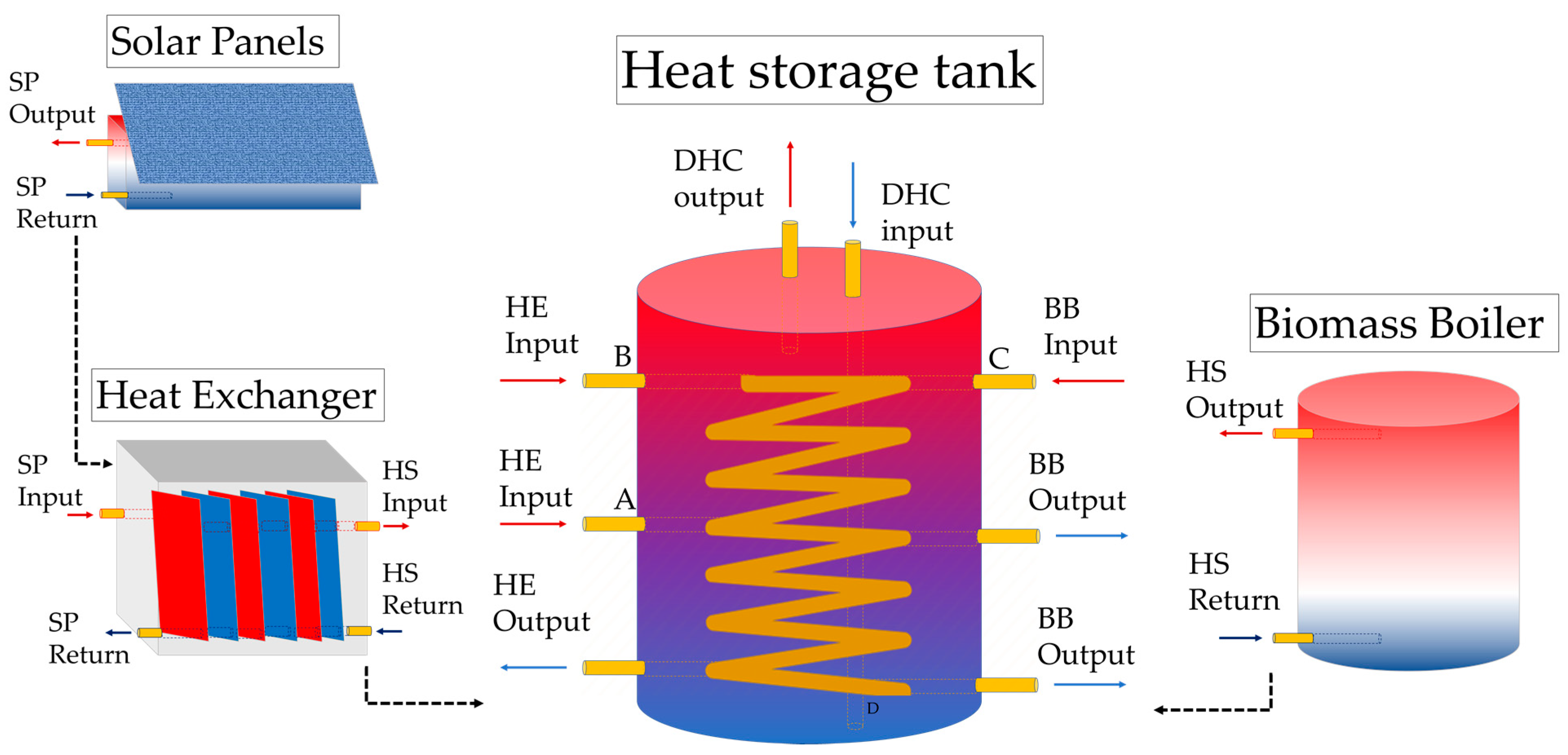
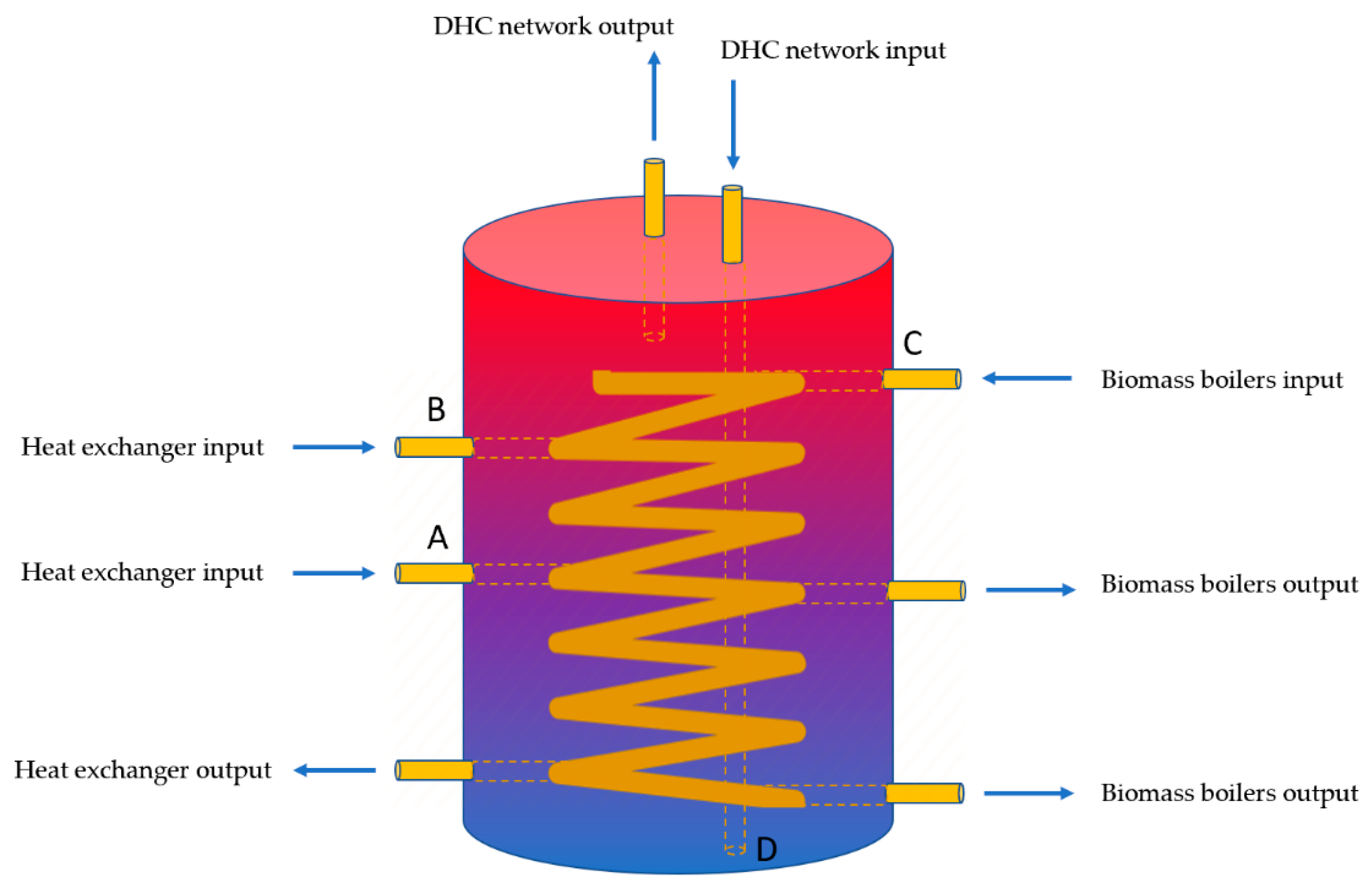
2.1. Problem Description
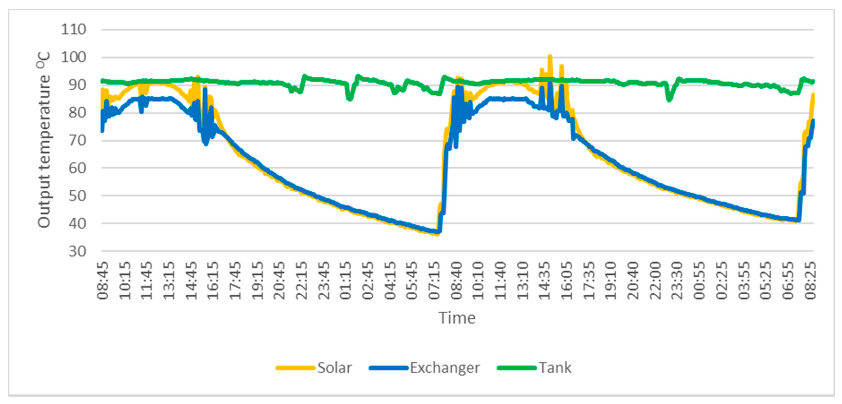
2.2. Data Acquisition and Characteristics
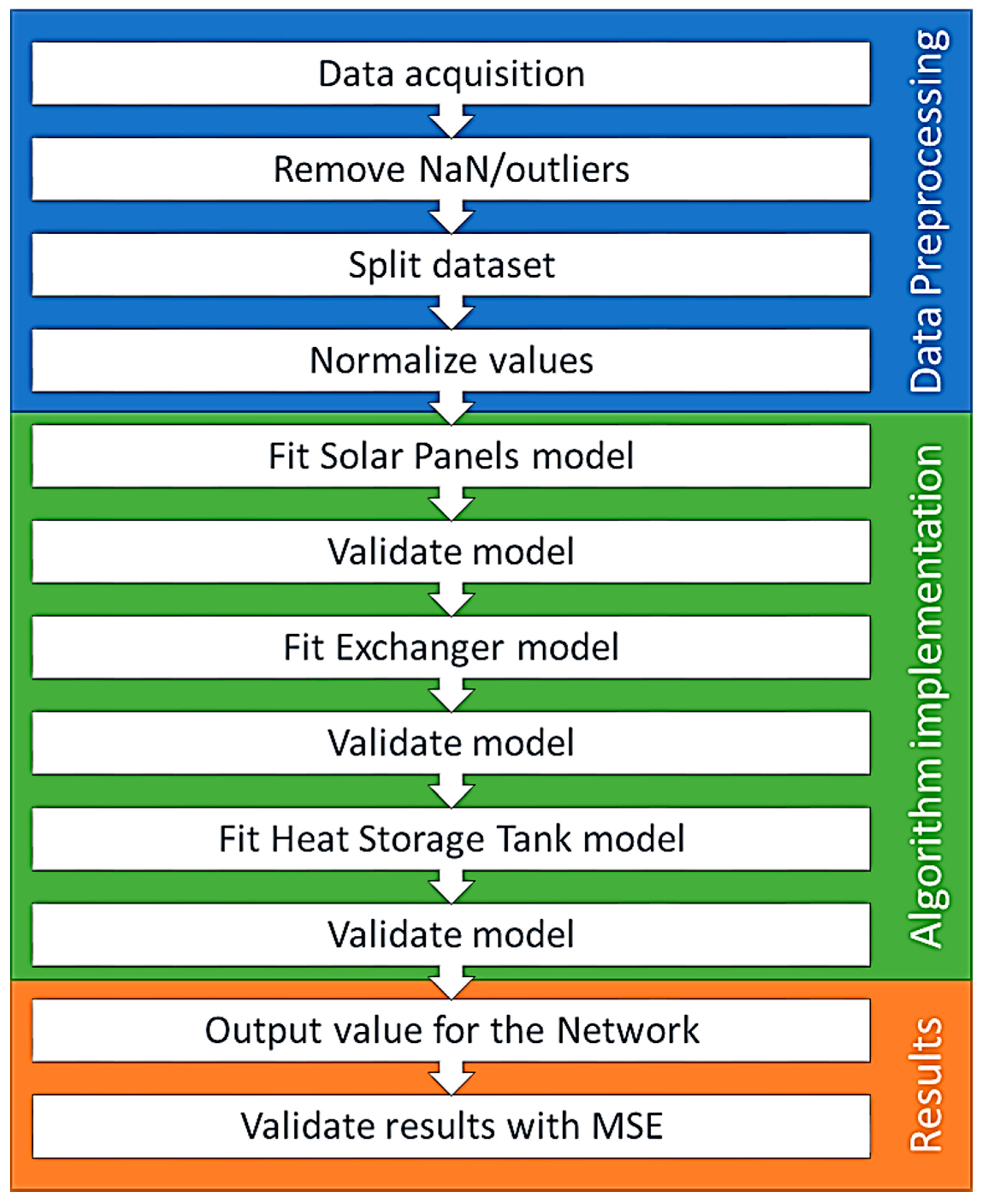
2.3. Preprocessing Phase
2.4. Proposed LSTM Architecture
2.5. Benchmarking Machine Learning Algorithms
2.6. Modelling Approaches: Component-Specific and Cascading
3. Results
3.1. Experimental Design
3.2. Performance of The Individual Modelling Approaches for Each Component
3.3. Performance of the Cascading Architecture
4. Discussion
5. Conclusions
Author Contributions
Funding
Data Availability Statement
Acknowledgments
Conflicts of Interest
References
- Reynolds, J.; Ahmad, M.W.; Rezgui, Y. Holistic modelling techniques for the operational optimisation of multi-vector energy systems. Energy Build. 2018, 169, 397–416. [Google Scholar] [CrossRef]
- Ayele, G.T.; Haurant, P.; Laumert, B.; Lacarrière, B. An extended energy hub approach for load flow analysis of highly coupled district energy networks: Illustration with electricity and heating. Appl. Energy 2018, 212, 850–867. [Google Scholar] [CrossRef]
- Nassif, A.B.; Azzeh, M.; Banitaan, S.; Neagu, D. Guest editorial: Special issue on predictive analytics using machine learning. Neural Comput. Appl. 2016, 27, 2153–2155. [Google Scholar] [CrossRef][Green Version]
- Bayes, T. An Essay towards Solving a Problem in the Doctrines of Chances. Philos. Trans. 1763, 45, 296–315. [Google Scholar] [CrossRef]
- Lecun, Y.; Bengio, Y.; Hinton, G. Deep learning. Nature 2015, 521, 436–444. [Google Scholar] [CrossRef]
- Ntakolia, C.; Anagnostis, A.; Moustakidis, S.; Karcanias, N. Machine learning applied on the district heating and cooling sector: A review. Energy Syst. 2021, 13, 1–30. [Google Scholar] [CrossRef]
- Kalogirou, S.A. Applications of artificial neural-networks for energy systems. Appl. Energy 2000, 67, 17–35. [Google Scholar] [CrossRef]
- Afram, A.; Janabi-Sharifi, F. Theory and applications of HVAC control systems—A review of model predictive control (MPC). Build. Environ. 2014, 72, 343–355. [Google Scholar] [CrossRef]
- Mohanraj, M.; Jayaraj, S.; Muraleedharan, C. Applications of artificial neural networks for thermal analysis of heat exchangers—A review. Int. J. Therm. Sci. 2015, 90, 150–172. [Google Scholar] [CrossRef]
- Yildiz, B.; Bilbao, J.I.; Sproul, A.B. A review and analysis of regression and machine learning models on commercial building electricity load forecasting. Renew. Sustain. Energy Rev. 2017, 73, 1104–1122. [Google Scholar] [CrossRef]
- Idowu, S.; Saguna, S.; Åhlund, C.; Schelén, O. Applied machine learning: Forecasting heat load in district heating system. Energy Build. 2016, 133, 478–488. [Google Scholar] [CrossRef]
- Mena, R.; Rodríguez, F.; Castilla, M.; Arahal, M.R. A prediction model based on neural networks for the energy consumption of a bioclimatic building. Energy Build. 2014, 82, 142–155. [Google Scholar] [CrossRef]
- Henze, G.; Schoenmann, J. Evaluation of Reinforcement Learning Control for Thermal Energy Storage Systems. HVAC R Res. 2003, 9, 259–275. [Google Scholar]
- Yokoyama, R.; Wakui, T.; Satake, R. Prediction of energy demands using neural network with model identification by global optimization. Energy Convers. Manag. 2009, 50, 319–327. [Google Scholar] [CrossRef]
- Luo, N.; Hong, T.; Li, H.; Jia, R.; Weng, W. Data analytics and optimization of an ice-based energy storage system for commercial buildings. Appl. Energy 2017, 204, 459–475. [Google Scholar] [CrossRef]
- Henze, G.P. An Overview of Optimal Control for Central Cooling Plants with Ice Thermal Energy Storage. J. Sol. Energy Eng. 2003, 125, 302. [Google Scholar] [CrossRef]
- Yaïci, W.; Entchev, E. Performance prediction of a solar thermal energy system using artificial neural networks. Appl. Therm. Eng. 2014, 73, 1348–1359. [Google Scholar] [CrossRef]
- Chou, J.S.; Bui, D.K. Modeling heating and cooling loads by artificial intelligence for energy-efficient building design. Energy Build. 2014, 82, 437–446. [Google Scholar] [CrossRef]
- Ben-Nakhi, A.E.; Mahmoud, M.A. Cooling load prediction for buildings using general regression neural networks. Energy Convers. Manag. 2004, 45, 2127–2141. [Google Scholar] [CrossRef]
- Kalogirou, S.A. Optimization of solar systems using artificial neural-networks and genetic algorithms. Appl. Energy 2004, 77, 383–405. [Google Scholar] [CrossRef]
- Abokersh, M.H.; Vallès, M.; Cabeza, L.F.; Boer, D. A framework for the optimal integration of solar assisted district heating in different urban sized communities: A robust machine learning approach incorporating global sensitivity analysis. Appl. Energy 2020, 267, 114903. [Google Scholar] [CrossRef]
- Dalipi, F.; Yildirim Yayilgan, S.; Gebremedhin, A. Data-Driven Machine-Learning Model in District Heating System for Heat Load Prediction: A Comparison Study. Appl. Comput. Intell. Soft Comput. 2016, 2016, 3403150. [Google Scholar] [CrossRef]
- Vlachopoulou, M.; Chin, G.; Fuller, J.C.J.C.; Lu, S.; Kalsi, K. Model for aggregated water heater load using dynamic bayesian networks. Proc. Int. Conf. Data Sci. 2012, 1, 818–823. [Google Scholar]
- Sajjadi, S.; Shamshirband, S.; Alizamir, M.; Yee, P.L.; Mansor, Z.; Manaf, A.A.; Altameem, T.A.; Mostafaeipour, A. Extreme learning machine for prediction of heat load in district heating systems. Energy Build. 2016, 122, 222–227. [Google Scholar] [CrossRef]
- Yaïci, W.; Entchev, E. Adaptive Neuro-Fuzzy Inference System modelling for performance prediction of solar thermal energy system. Renew. Energy 2016, 86, 302–315. [Google Scholar] [CrossRef]
- Chia, Y.Y.; Lee, L.H.; Shafiabady, N.; Isa, D. A load predictive energy management system for supercapacitor-battery hybrid energy storage system in solar application using the Support Vector Machine. Appl. Energy 2015, 137, 588–602. [Google Scholar] [CrossRef]
- Johansson, C.; Bergkvist, M.; Geysen, D.; De Somer, O.; Lavesson, N.; Vanhoudt, D. Operational Demand Forecasting in District Heating Systems Using Ensembles of Online Machine Learning Algorithms. Energy Procedia 2017, 116, 208–216. [Google Scholar] [CrossRef]
- Moustakidis, S.; Meintanis, I.; Halikias, G.; Karcanias, N. An innovative control framework for district heating systems: Conceptualisation and preliminary results. Resources 2019, 8, 27. [Google Scholar] [CrossRef]
- Moustakidis, S.; Meintanis, I.; Karkanias, N.; Halikias, G.; Saoutieff, E.; Gasnier, P.; Ojer-Aranguren, J.; Anagnostis, A.; Marciniak, B.; Rodot, I.; et al. Innovative Technologies for District Heating and Cooling: InDeal Project. Proceedings 2019, 5, 1. [Google Scholar] [CrossRef]
- Popa, D.; Pop, F.; Serbanescu, C.; Castiglione, A. Deep learning model for home automation and energy reduction in a smart home environment platform. Neural Comput. Appl. 2018, 31, 1317–1337. [Google Scholar] [CrossRef]
- Vázquez-Canteli, J.R.; Ulyanin, S.; Kämpf, J.; Nagy, Z. Fusing TensorFlow with building energy simulation for intelligent energy management in smart cities. Sustain. Cities Soc. 2019, 45, 243–257. [Google Scholar] [CrossRef]
- Sogabe, T.; Malla, D.B.; Takayama, S.; Shin, S.; Sakamoto, K.; Yamaguchi, K.; Singh, T.P.; Sogabe, M.; Hirata, T.; Okada, Y. Smart Grid Optimization by Deep Reinforcement Learning over Discrete and Continuous Action Space. In Proceedings of the 2018 IEEE 7th World Conference on Photovoltaic Energy Conversion, WCPEC 2018—A Joint Conference of 45th IEEE PVSC, 28th PVSEC and 34th EU PVSEC, Waikoloa, HI, USA, 10–15 June 2018. [Google Scholar]
- Cox, S.J.; Kim, D.; Cho, H.; Mago, P. Real time optimal control of district cooling system with thermal energy storage using neural networks. Appl. Energy 2019, 238, 466–480. [Google Scholar] [CrossRef]
- Rahman, A.; Smith, A.D. Predicting heating demand and sizing a stratified thermal storage tank using deep learning algorithms. Appl. Energy 2018, 228, 108–121. [Google Scholar] [CrossRef]
- Le Coz, A.; Nabil, T.; Courtot, F. Towards optimal district heating temperature control in China with deep reinforcement learning. arXiv 2020, arXiv:2012.09508. [Google Scholar]
- Xue, G.; Pan, Y.; Lin, T.; Song, J.; Qi, C.; Wang, Z. District heating load prediction algorithm based on feature fusion LSTM model. Energies 2019, 12, 2122. [Google Scholar] [CrossRef]
- Gong, M.; Zhou, H.; Wang, Q.; Wang, S.; Yang, P. District heating systems load forecasting: A deep neural networks model based on similar day approach. Adv. Build. Energy Res. 2019, 14, 372–388. [Google Scholar] [CrossRef]
- Ullah, A.; Haydarov, K.; Haq, I.U.; Muhammad, K.; Rho, S.; Lee, M.; Baik, S.W. Deep learning assisted buildings energy consumption profiling using smart meter data. Sensors 2020, 20, 873. [Google Scholar] [CrossRef]
- Corberan, J.M.; Finn, D.P.; Montagud, C.M.; Murphy, F.T.; Edwards, K.C. A quasi-steady state mathematical model of an integrated ground source heat pump for building space control. Energy Build. 2011, 43, 82–92. [Google Scholar] [CrossRef]
- Petrocelli, D.; Lezzi, A.M. Modeling operation mode of pellet boilers for residential heating. Proc. J. Phys. Conf. Ser. 2014, 547, 012017. [Google Scholar] [CrossRef]
- Campos Celador, A.; Odriozola, M.; Sala, J.M. Implications of the modelling of stratified hot water storage tanks in the simulation of CHP plants. Energy Convers. Manag. 2011, 52, 3018–3026. [Google Scholar] [CrossRef]
- Shin, M.S.; Kim, H.S.; Jang, D.S.; Lee, S.N.; Lee, Y.S.; Yoon, H.G. Numerical and experimental study on the design of a stratified thermal storage system. Appl. Therm. Eng. 2004, 24, 17–27. [Google Scholar] [CrossRef]
- Montes, M.J.; Abánades, A.; Martínez-Val, J.M. Thermofluidynamic Model and Comparative Analysis of Parabolic Trough Collectors Using Oil, Water/Steam, or Molten Salt as Heat Transfer Fluids. J. Sol. Energy Eng. 2010, 132, 021001. [Google Scholar] [CrossRef]
- Duffie, J.A.; Beckman, W.A. Solar Engineering of Thermal Processes: Fourth Edition; Wiley: New York, NY, USA, 2013; ISBN 9780470873663. [Google Scholar]
- Notton, G.; Motte, F.; Cristofari, C.; Canaletti, J.L. New patented solar thermal concept for high building integration: Test and modeling. Energy Procedia 2013, 42, 43–52. [Google Scholar] [CrossRef]
- Dowson, M.; Pegg, I.; Harrison, D.; Dehouche, Z. Predicted and in situ performance of a solar air collector incorporating a translucent granular aerogel cover. Energy Build. 2012, 49, 173–187. [Google Scholar] [CrossRef]
- Karim, M.A.; Perez, E.; Amin, Z.M. Mathematical modelling of counter flow v-grove solar air collector. Renew. Energy 2014, 67, 192–201. [Google Scholar] [CrossRef]
- Géczy-Víg, P.; Farkas, I. Neural network modelling of thermal stratification in a solar DHW storage. Sol. Energy 2010, 84, 801–806. [Google Scholar] [CrossRef]
- Caner, M.; Gedik, E.; Keĉebaŝ, A. Investigation on thermal performance calculation of two type solar air collectors using artificial neural network. Expert Syst. Appl. 2011, 38, 1668–1674. [Google Scholar] [CrossRef]
- Sözen, A.; Menlik, T.; Ünvar, S. Determination of efficiency of flat-plate solar collectors using neural network approach. Expert Syst. Appl. 2008, 35, 1533–1539. [Google Scholar] [CrossRef]
- Esen, H.; Ozgen, F.; Esen, M.; Sengur, A. Artificial neural network and wavelet neural network approaches for modelling of a solar air heater. Expert Syst. Appl. 2009, 36, 11240–11248. [Google Scholar] [CrossRef]
- Liu, Z.; Li, H.; Zhang, X.; Jin, G.; Cheng, K. Novel method for measuring the heat collection rate and heat loss coefficient of water-in-glass evacuated tube solar water heaters based on artificial neural networks and support vector machine. Energies 2015, 8, 8814–8834. [Google Scholar] [CrossRef]
- García Nieto, P.J.; García-Gonzalo, E.; Paredes-Sánchez, J.P.; Bernardo Sánchez, A.; Menéndez Fernández, M. Predictive modelling of the higher heating value in biomass torrefaction for the energy treatment process using machine-learning techniques. Neural Comput. Appl. 2018, 31, 8823–8836. [Google Scholar] [CrossRef]
- Kalogirou, S.; Lalot, S.; Florides, G.; Desmet, B. Development of a neural network-based fault diagnostic system for solar thermal applications. Sol. Energy 2008, 82, 164–172. [Google Scholar] [CrossRef]
- Ahmad, M.W.; Mourshed, M.; Yuce, B.; Rezgui, Y. Computational intelligence techniques for HVAC systems: A review. Build. Simul. 2016, 9, 359–398. [Google Scholar] [CrossRef]
- Kalogirou, S.A.; Mathioulakis, E.; Belessiotis, V. Artificial neural networks for the performance prediction of large solar systems. Renew. Energy 2014, 63, 90–97. [Google Scholar] [CrossRef]
- Energetika Project. Available online: http://www.energetika-projekt.eu (accessed on 11 January 2019).
- Anagnostis, A.; Papageorgiou, E.; Bochtis, D. Application of artificial neural networks for natural gas consumption forecasting. Sustainability 2020, 12, 6409. [Google Scholar] [CrossRef]
- Anagnostis, A.; Papageorgiou, E.; Dafopoulos, V.; Bochtis, D. Applying Long Short-Term Memory Networks for natural gas demand prediction. In Proceedings of the 2019 10th International Conference on Information, Intelligence, Systems and Applications (IISA), Patras, Greece, 15–17 July 2019; pp. 1–7. [Google Scholar]
- Hochreiter, S. The vanishing gradient problem during learning recurrent neural nets and problem solutions. Int. J. Uncertain. Fuzziness Knowl.-Based Syst. 1998, 6, 107–116. [Google Scholar] [CrossRef]
- Hochreiter, S.; Schmidhuber, J. Long Short-Term Memory. Neural Comput. 1997, 9, 1735–1780. [Google Scholar] [CrossRef]
- Galton, F. Anthropological Miscellanea. Regression towards Mediocrity in Iiereditary Stature. J. Anthropol. Inst. Great Br. Irel. 1886, 15, 246–263. [Google Scholar]
- Santosa, F.; Symes, W.W. Linear Inversion of Band-Limited Reflection Seismograms. SIAM J. Sci. Stat. Comput. 1986, 7, 1307–1330. [Google Scholar] [CrossRef]
- Tibshirani, R. Regression Selection and Shrinkage via the Lasso. J. R. Stat. Soc. B 1996, 58, 267–288. [Google Scholar] [CrossRef]
- Pasanen, L.; Holmström, L.; Sillanpää, M.J. Bayesian LASSO, scale space and decision making in association genetics. PLoS ONE 2015, 10, e0120017. [Google Scholar] [CrossRef] [PubMed]
- De Mol, C.; De Vito, E.; Rosasco, L. Elastic-net regularization in learning theory. J. Complex. 2009, 25, 201–230. [Google Scholar] [CrossRef]
- Efron, B.; Hastie, T.; Johnstone, I.; Tibshirani, R.; Ishwaran, H.; Knight, K.; Loubes, J.M.; Massart, P.; Madigan, D.; Ridgeway, G.; et al. Least angle regression. Ann. Stat. 2004, 32, 407–499. [Google Scholar] [CrossRef]
- Robbins, H.; Monro, S. A Stochastic Approximation Method. IEEE Trans. Syst. Man Cybern. 1971, 1, 338–344. [Google Scholar]
- Belson, W.A. Matching and Prediction on the Principle of Biological Classification; Wiley: New York, NY, USA, 1959; Volume 8, ISBN 0000000779. [Google Scholar]
- Breiman, L.; Friedman, J.H.; Olshen, R.A.; Stone, C.J. Classification and Regression Trees; Routledge: New York, NY, USA, 2017; ISBN 9781351460491. [Google Scholar] [CrossRef]
- Breiman, L. Random forests. Mach. Learn. 2001, 45, 5–32. [Google Scholar] [CrossRef]
- Freund, Y.; Schapire, R.; Abe, N. A Short Introduction to Boosting. J. Jpn. Soc. Artif. Intell. 1999, 14, 1612. [Google Scholar]
- Freund, Y.; Schapire, R.R.E. Experiments with a New Boosting Algorithm. In Proceedings of the 13th International Conference on Machine Learning, Bari, Italy, 3–6 July 1996. [Google Scholar]
- Breiman, L. Bagging predictors. Mach. Learn. 1996, 24, 123–140. [Google Scholar] [CrossRef]
- Vapnik, V.N. An overview of statistical learning theory. IEEE Trans. Neural Netw. 1999, 10, 988–999. [Google Scholar] [CrossRef]
- Suykens, J.A.K.; Vandewalle, J. Least squares support vector machine classifiers. Neural Process. Lett. 1999, 9, 293–300. [Google Scholar] [CrossRef]
- Chang, C.; Lin, C.; Tieleman, T. LIBSVM: A Library for Support Vector Machines. ACM Trans. Intell. Syst. Technol. 2008, 2, 1–27. [Google Scholar] [CrossRef]
- McCulloch, W.S.; Pitts, W. A logical calculus of the ideas immanent in nervous activity. Bull. Math. Biophys. 1943, 5, 115–133. [Google Scholar] [CrossRef]
- Rosenblatt, F. The perceptron: A probabilistic model for information storage and organization in the brain. Psychol. Rev. 1958, 65, 386. [Google Scholar] [CrossRef] [PubMed]
- Pal, S.K.; Mitra, S. Multilayer Perceptron, Fuzzy Sets, and Classification. IEEE Trans. Neural Netw. 1992, 3, 683–697. [Google Scholar] [CrossRef] [PubMed]
- Linnainmaa, S. Taylor expansion of the accumulated rounding error. BIT 1976, 16, 146–160. [Google Scholar] [CrossRef]
- Riedmiller, M.; Braun, H. A direct adaptive method for faster backpropagation learning: The RPROP algorithm. In Proceedings of the IEEE International Conference on Neural Networks—Conference Proceedings, Nagoya, Japan, 25–29 October 1993. [Google Scholar]
- Broomhead, D.; Lowe, D. Multivariable functional interpolation and adaptive networks. Complex Syst. 1988, 2, 321–355. [Google Scholar]
- McClelland, J.L.; Rumelhart, D.E.; McClelland, J.L. Parallel Distributed Processing: Explorations in the Microstructure of Cognition, Volume 2: Psychological and Biological Models; The MIT Press: Boston, MA, USA, 1986; ISBN 0262132184. [Google Scholar]
- Jang, J.S.R. ANFIS: Adaptive-Network-Based Fuzzy Inference System. IEEE Trans. Syst. Man Cybern. 1993, 23, 665–685. [Google Scholar] [CrossRef]
- Jordan, M.I. Attractor dynamics and parallelism in a connectionist sequential machine. In Proceedings of the Eighth Annual Conference Cognitive Science Society, Amhurst, MA, USA, 15–17 August 1986; pp. 531–546. [Google Scholar]
- Fukushima, K. Neocognitron: A self-organizing neural network model for a mechanism of pattern recognition unaffected by shift in position. Biol. Cybern. 1980, 36, 193–202. [Google Scholar] [CrossRef]
- Ivakhnenko, A.G. Polynomial Theory of Complex Systems. IEEE Trans. Syst. Man Cybern. 1971, 4, 364–378. [Google Scholar] [CrossRef]
- Nair, V.; Hinton, G.E. Rectified linear units improve Restricted Boltzmann machines. In Proceedings of the ICML 2010—Proceedings, 27th International Conference on Machine Learning, Haifa, Israel, 21–24 June 2010. [Google Scholar]
- Kingma, D.P.; Ba, J.L. Adam: A method for stochastic optimization. In Proceedings of the 3rd International Conference on Learning Representations, ICLR 2015—Conference Track Proceedings, San Diego, CA, USA, 7–9 May 2015. [Google Scholar]
- Harris, C.R.; Millman, K.J.; van der Walt, S.J.; Gommers, R.; Virtanen, P.; Cournapeau, D.; Wieser, E.; Taylor, J.; Berg, S.; Smith, N.J.; et al. Array programming with NumPy. Nature 2020, 585, 357–362. [Google Scholar] [CrossRef]
- McKinney, W. Data Structures for Statistical Computing in Python. In Proceedings of the 9th Python in Science Conference, Austin, TX, USA, 28 June–3 July 2010. [Google Scholar]
- Hunter, J.D. Matplotlib: A 2D graphics environment. Comput. Sci. Eng. 2007, 9, 90–95. [Google Scholar] [CrossRef]
- Pedregosa, F.; Varoquaux, G.; Gramfort, A.; Michel, V.; Thirion, B.; Grisel, O.; Blondel, M.; Prettenhofer, P.; Weiss, R.; Dubourg, V.; et al. Scikit-learn: Machine learning in Python. J. Mach. Learn. Res. 2011, 12, 2825–2830. [Google Scholar]
- Chollet, F. Others Keras. 2015. Available online: https://github.com/fchollet/keras (accessed on 11 January 2019).
- Abadi, M.; Agarwal, A.; Barham, P.; Brevdo, E.; Chen, Z.; Citro, C.; Corrado, G.S.; Davis, A.; Dean, J.; Devin, M.; et al. TensorFlow: Large-Scale Machine Learning on Heterogeneous Distributed Systems. arXiv 2016, arXiv:1603.04467. [Google Scholar]
- Kiseľák, J.; Lu, Y.; Švihra, J.; Szépe, P.; Stehlík, M. “SPOCU”: Scaled polynomial constant unit activation function. Neural Comput. Appl. 2020, 33, 3385–3401. [Google Scholar] [CrossRef]


| Feature Name | Solar Panels | Heat Exchanger | Heat Storage Tank |
|---|---|---|---|
| T1 Solar collector field 1 (°C) | Input | - | - |
| T2 Solar collector field 2 (°C) | Input | - | - |
| T3 Solar collector field 3 (°C) | Input | - | - |
| T4 Solar collector field 4 (°C) | Input | - | - |
| T5 Solar collector field 5 (°C) | Input | - | - |
| T6 Solar collector field 6 (°C) | Input | - | - |
| T7 Solar collector field 7 (°C) | Input | - | - |
| T8 feed-in Solar prim. (°C) | Output | Input | - |
| T9 return Solar prim. (°C) | Return Input | Input | - |
| T10 feed-in Solar sec. (°C) | - | Output | Input |
| T11 return Solar sec. (°C) | - | Return Input | - |
| T12 Temp. 1 heat storage (up) (°C) | - | - | Input |
| T13 Temp. 2 heat storage (°C) | - | - | Input |
| T14 Temp. 3 heat storage (°C) | - | - | Input |
| T15 Temp. 4 heat storage (°C) | - | - | Input |
| T16 Temp. 5 heat storage (°C) | - | - | Input |
| T17 feed-in biomass boiler (°C) | - | - | Input |
| T18 return biomass boiler (°C) | - | - | Input |
| T19 feed-in before mixing valve (°C) | - | - | Output |
| T20 return before mixing valve (°C) | - | - | Return Input |
| T21 outside temp. (°C) | Universal Input | ||
| Total number of training samples multiplied by the features of each component | 3,511,480 | 1,755,740 | 3,862,628 |
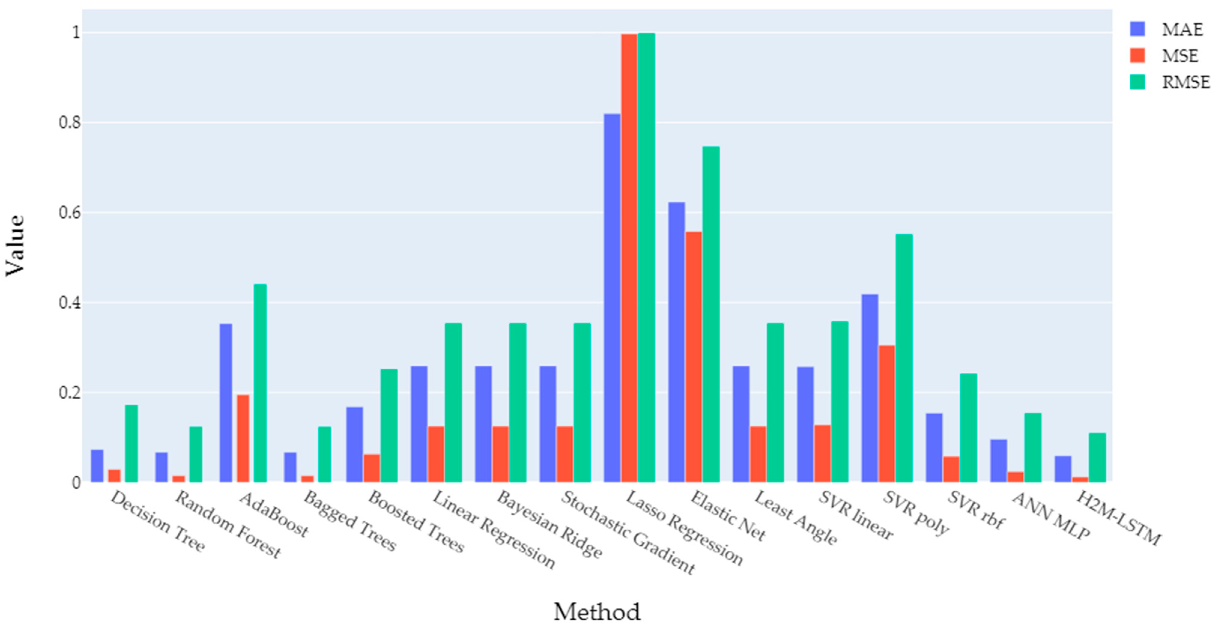
| Method | MAE | MSE | RMSE |
|---|---|---|---|
| Decision Tree | 0.073 | 0.029 | 0.172 |
| Random Forest | 0.067 | 0.015 | 0.124 |
| AdaBoost | 0.353 | 0.195 | 0.441 |
| Bagged Trees | 0.067 | 0.015 | 0.124 |
| Boosted Trees | 0.168 | 0.063 | 0.252 |
| Linear Regression | 0.259 | 0.125 | 0.354 |
| Bayesian Ridge | 0.259 | 0.125 | 0.354 |
| Stochastic Gradient | 0.259 | 0.125 | 0.354 |
| Lasso Regression | 0.820 | 0.997 | 0.999 |
| Elastic Net | 0.623 | 0.558 | 0.747 |
| Least Angle | 0.259 | 0.125 | 0.354 |
| SVR linear | 0.257 | 0.128 | 0.358 |
| SVR poly | 0.419 | 0.305 | 0.552 |
| SVR rbf | 0.154 | 0.058 | 0.242 |
| ANN MLP | 0.096 | 0.024 | 0.154 |
| H2M-LSTM | 0.059 | 0.012 | 0.110 |
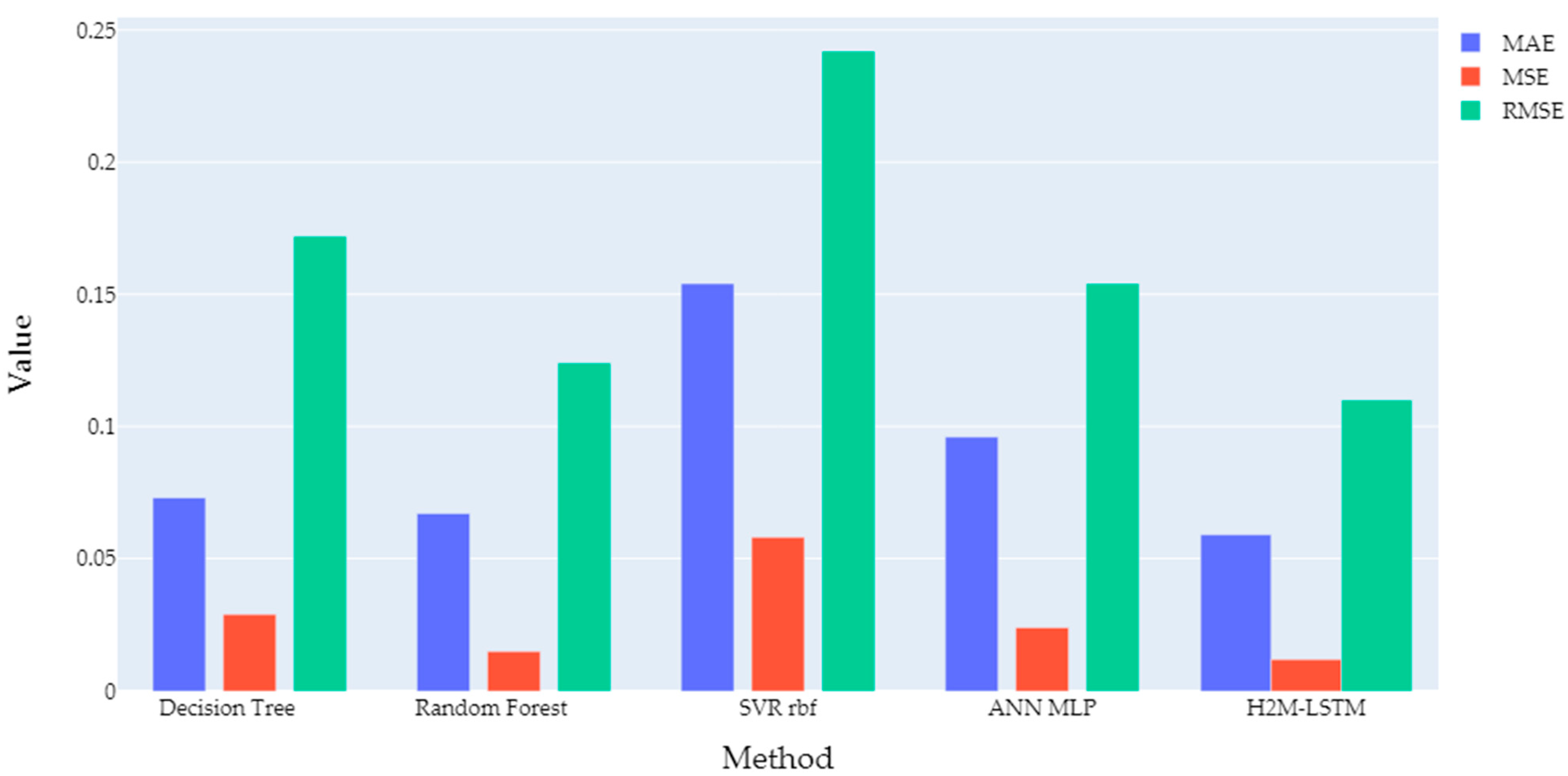
| Method | MAE | MSE | RMSE |
|---|---|---|---|
| Decision Tree | 0.026 | 0.005 | 0.069 |
| Random Forest | 0.023 | 0.003 | 0.055 |
| AdaBoost | 0.172 | 0.048 | 0.219 |
| Bagged Trees | 0.023 | 0.003 | 0.055 |
| Boosted Trees | 0.057 | 0.010 | 0.099 |
| Linear Regression | 0.081 | 0.019 | 0.136 |
| Bayesian Ridge | 0.081 | 0.019 | 0.136 |
| Stochastic Gradient | 0.081 | 0.019 | 0.136 |
| Lasso Regression | 0.830 | 0.998 | 0.999 |
| Elastic Net | 0.525 | 0.396 | 0.629 |
| Least Angle | 0.081 | 0.019 | 0.136 |
| SVR linear | 0.082 | 0.019 | 0.139 |
| SVR poly | 0.361 | 0.718 | 0.847 |
| SVR rbf | 0.059 | 0.008 | 0.091 |
| ANN MLP | 0.033 | 0.004 | 0.060 |
| H2M-LSTM | 0.020 | 0.002 | 0.045 |
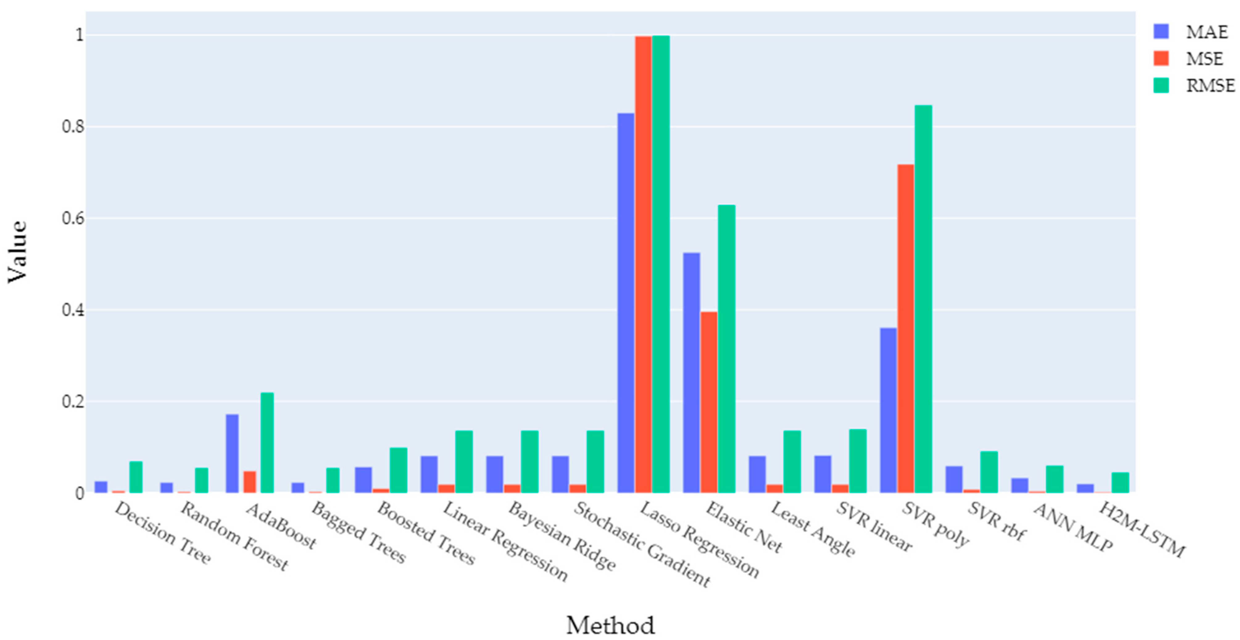
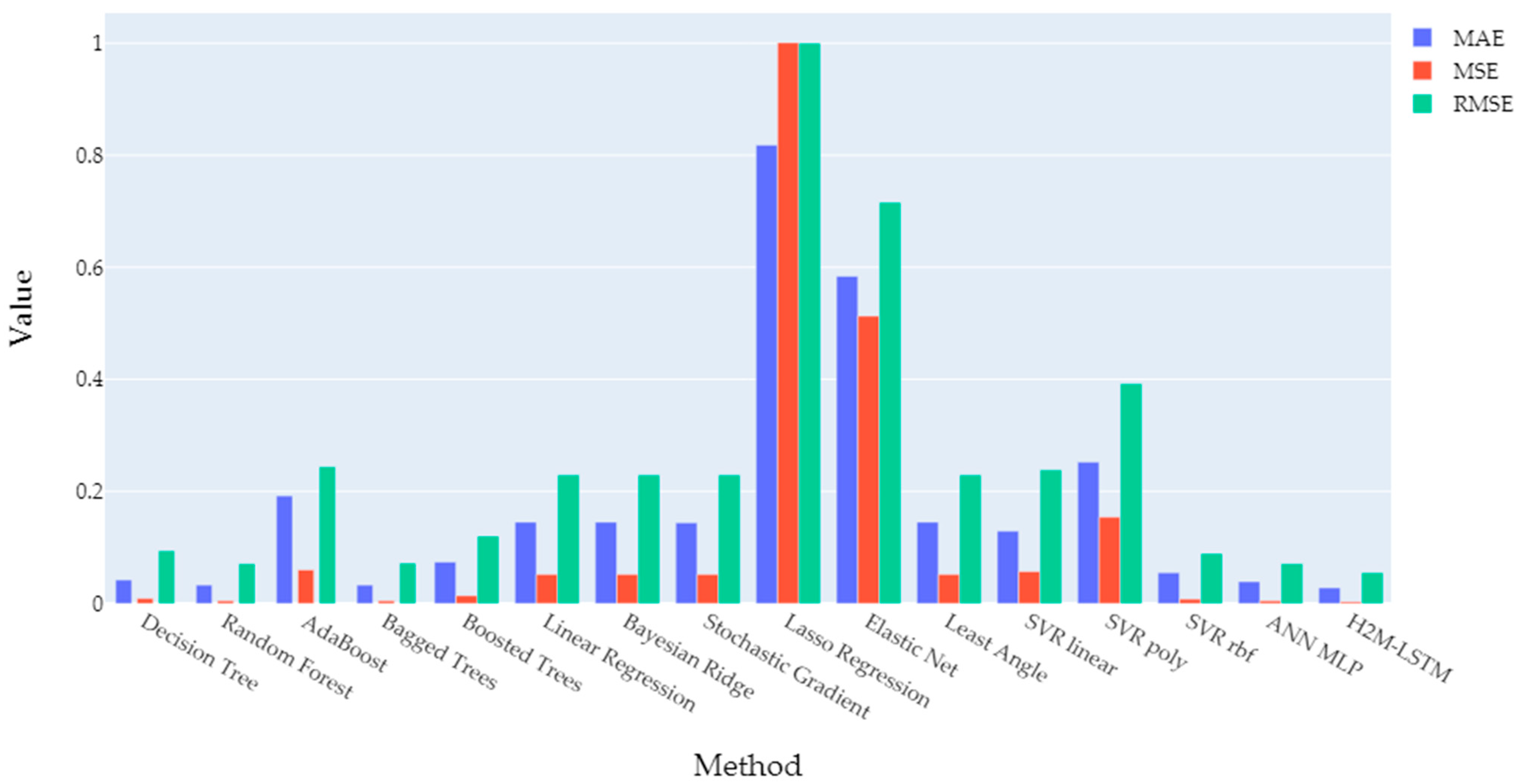
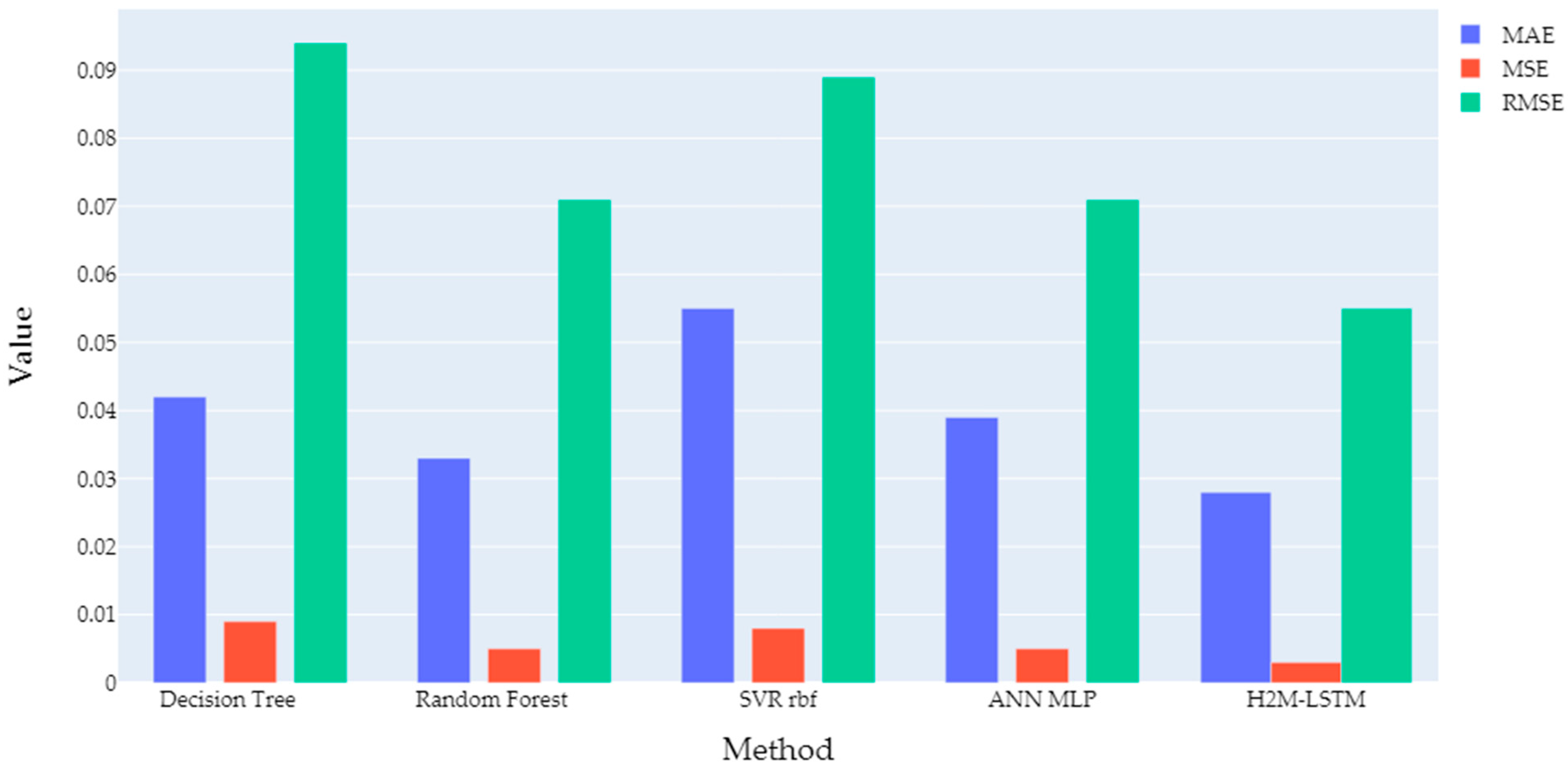
| Method | MAE | MSE | RMSE |
|---|---|---|---|
| Decision Tree | 0.042 | 0.009 | 0.094 |
| Random Forest | 0.033 | 0.005 | 0.071 |
| AdaBoost | 0.192 | 0.060 | 0.244 |
| Bagged Trees | 0.033 | 0.005 | 0.072 |
| Boosted Trees | 0.074 | 0.014 | 0.120 |
| Linear Regression | 0.145 | 0.052 | 0.229 |
| Bayesian Ridge | 0.145 | 0.052 | 0.229 |
| Stochastic Gradient | 0.144 | 0.052 | 0.229 |
| Lasso Regression | 0.818 | 1.001 | 1.000 |
| Elastic Net | 0.584 | 0.513 | 0.716 |
| Least Angle | 0.145 | 0.052 | 0.229 |
| SVR linear | 0.129 | 0.057 | 0.238 |
| SVR poly | 0.252 | 0.154 | 0.392 |
| SVR rbf | 0.055 | 0.008 | 0.089 |
| ANN MLP | 0.039 | 0.005 | 0.071 |
| H2M-LSTM | 0.028 | 0.003 | 0.055 |
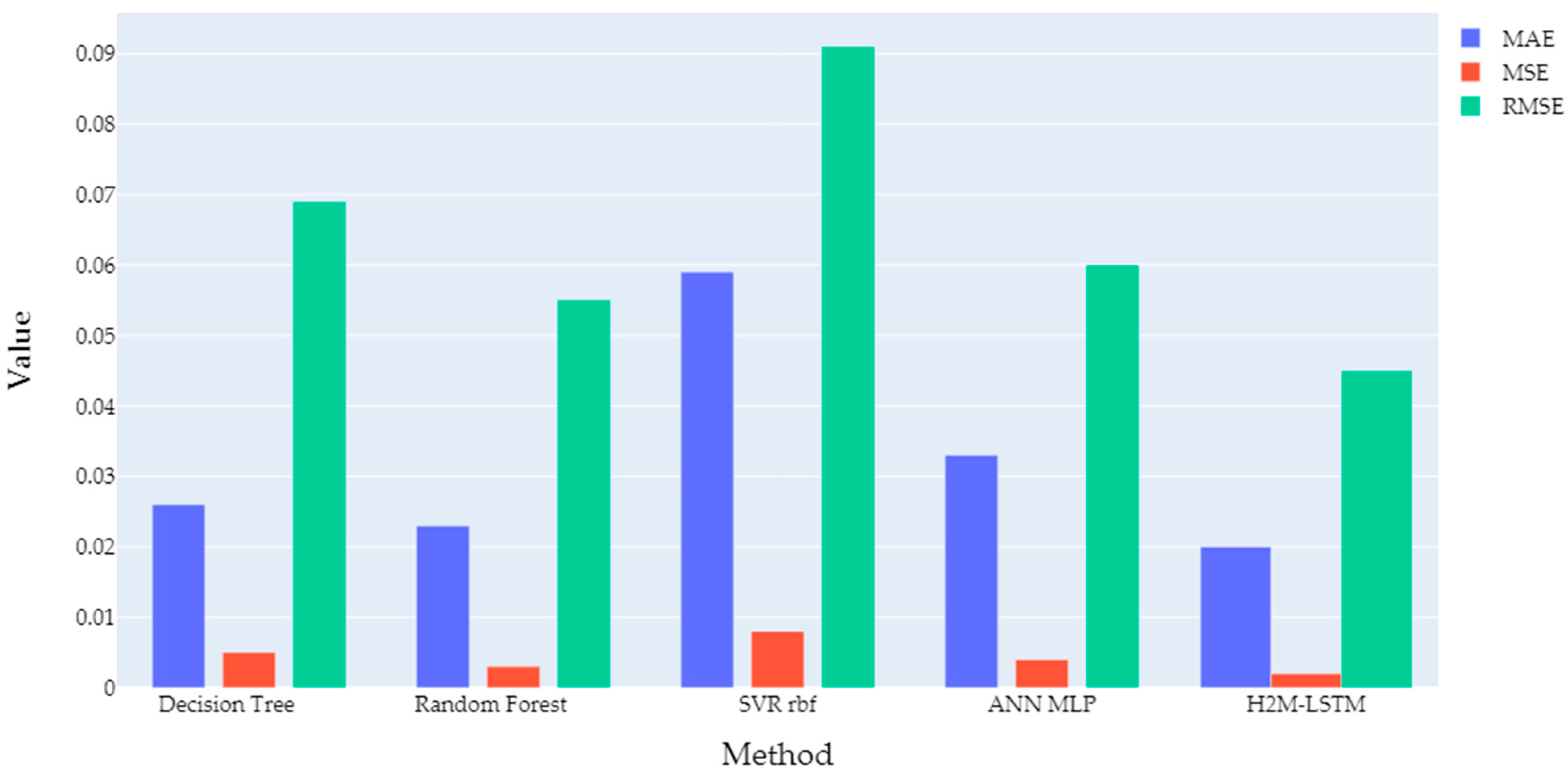
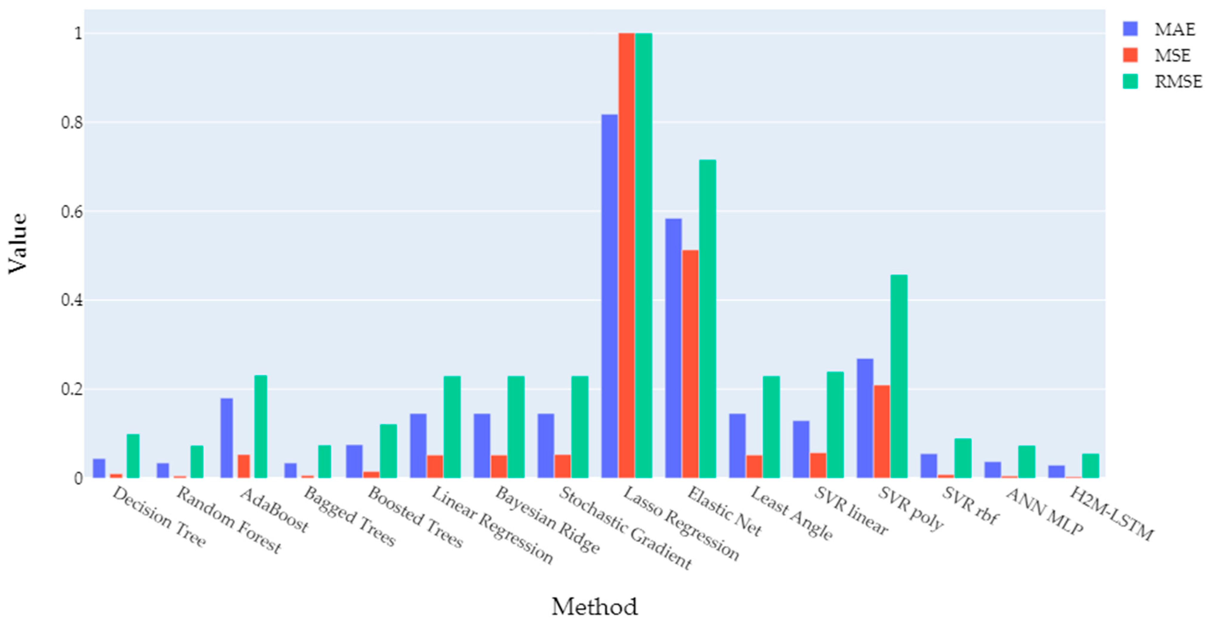
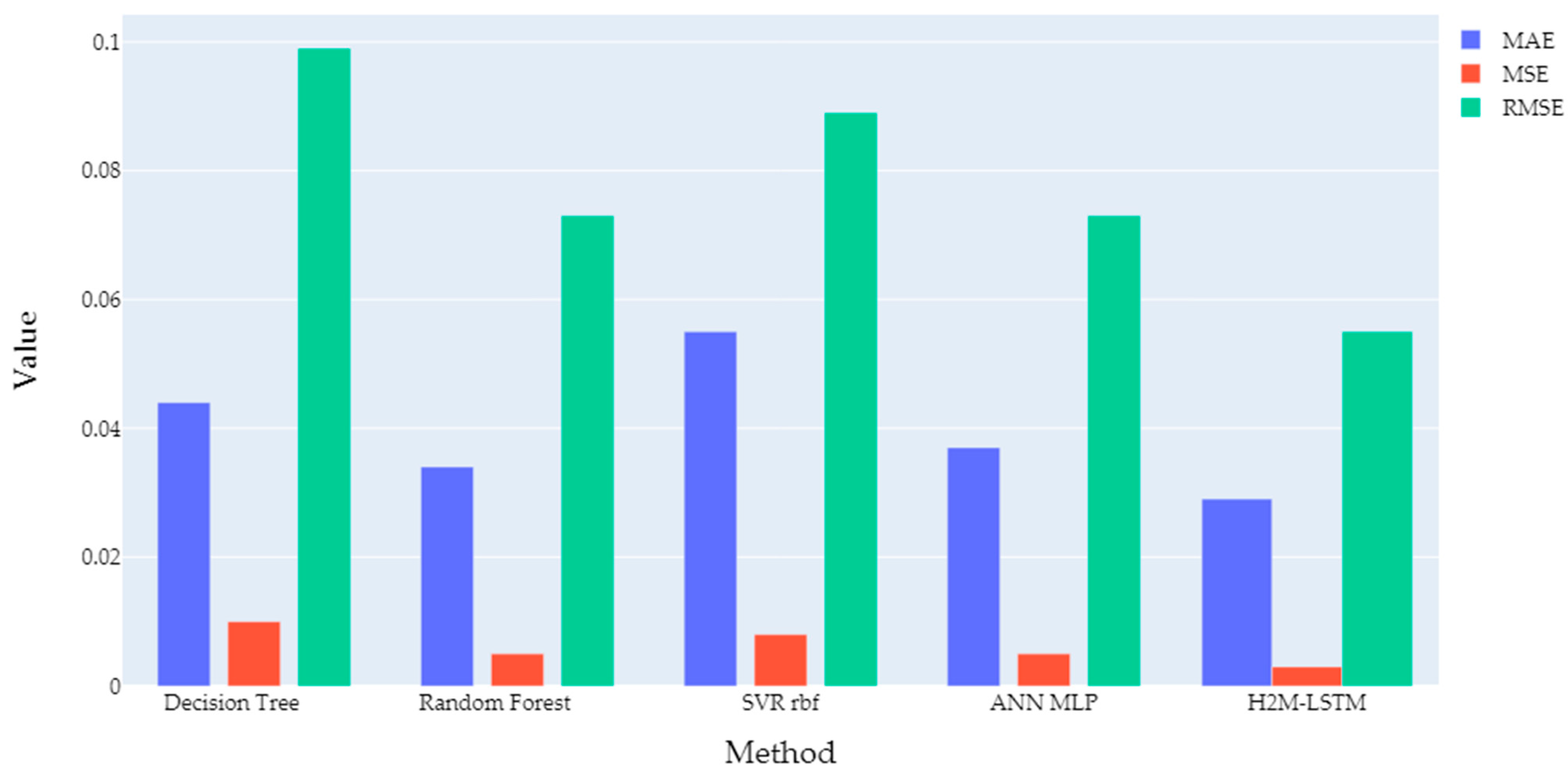
| Method | MAE | MSE | RMSE |
|---|---|---|---|
| Decision Tree | 0.044 | 0.010 | 0.099 |
| Random Forest | 0.034 | 0.005 | 0.073 |
| AdaBoost | 0.180 | 0.053 | 0.231 |
| Bagged Trees | 0.034 | 0.006 | 0.074 |
| Boosted Trees | 0.075 | 0.015 | 0.121 |
| Linear Regression | 0.145 | 0.052 | 0.229 |
| Bayesian Ridge | 0.145 | 0.052 | 0.229 |
| Stochastic Gradient | 0.145 | 0.053 | 0.229 |
| Lasso Regression | 0.818 | 1.001 | 1.000 |
| Elastic Net | 0.584 | 0.513 | 0.716 |
| Least Angle | 0.145 | 0.052 | 0.229 |
| SVR linear | 0.129 | 0.057 | 0.239 |
| SVR poly | 0.269 | 0.209 | 0.457 |
| SVR rbf | 0.055 | 0.008 | 0.089 |
| ANN MLP | 0.037 | 0.005 | 0.073 |
| H2M-LSTM | 0.029 | 0.003 | 0.055 |
Publisher’s Note: MDPI stays neutral with regard to jurisdictional claims in published maps and institutional affiliations. |
© 2022 by the authors. Licensee MDPI, Basel, Switzerland. This article is an open access article distributed under the terms and conditions of the Creative Commons Attribution (CC BY) license (https://creativecommons.org/licenses/by/4.0/).
Share and Cite
Anagnostis, A.; Moustakidis, S.; Papageorgiou, E.; Bochtis, D. A Hybrid Bimodal LSTM Architecture for Cascading Thermal Energy Storage Modelling. Energies 2022, 15, 1959. https://doi.org/10.3390/en15061959
Anagnostis A, Moustakidis S, Papageorgiou E, Bochtis D. A Hybrid Bimodal LSTM Architecture for Cascading Thermal Energy Storage Modelling. Energies. 2022; 15(6):1959. https://doi.org/10.3390/en15061959
Chicago/Turabian StyleAnagnostis, Athanasios, Serafeim Moustakidis, Elpiniki Papageorgiou, and Dionysis Bochtis. 2022. "A Hybrid Bimodal LSTM Architecture for Cascading Thermal Energy Storage Modelling" Energies 15, no. 6: 1959. https://doi.org/10.3390/en15061959
APA StyleAnagnostis, A., Moustakidis, S., Papageorgiou, E., & Bochtis, D. (2022). A Hybrid Bimodal LSTM Architecture for Cascading Thermal Energy Storage Modelling. Energies, 15(6), 1959. https://doi.org/10.3390/en15061959