On the Dynamic Connectedness of the Stock, Oil, Clean Energy, and Technology Markets

Abstract

Using monthly data from September 2004 to February 2020, this paper investigates the connectedness of the renewable energy, common stock, oil, and technology markets. The time-domain Diebold and Yilmaz spillover index approach is used to analyze the volatility spillover between these four markets. The study’s findings reveal that the oil and clean energy markets have bidirectional volatility spillover. The oil market has been found to be a net receiver of volatility. Furthermore, the study shows that volatility spillover is stronger in extreme positive and negative shock periods than in medium shock periods. Our findings show that, during crisis periods, the volatility spillover index rises, while the total connection reached its lowest point in 2015. Our findings suggest that policymakers should be informed that, as long as oil prices remain low, alternative energy-producing industries will not require specific policies to mitigate their vulnerability to crude oil price shocks. However, large spillover in the tails—particularly in the right tail—indicates vulnerability to extreme events, such as the negative effect of oil price increases.

1. Introduction

Economists have been urging policymakers to establish sustainable energy sectors in recent years to mitigate air pollution and balance the negative effects of oil price volatility, taking population growth and the demand for fossil fuels into account. Additionally, oil is a worldwide commodity, and its price is determined by the demand and supply situations. Thus, this rapidly growing demand for oil from emerging economies and a shortage in the oil supply will significantly increase oil prices and encourage investors to substitute oil with renewable energy.

Furthermore, the prospects for oil are complex over the near–medium term, since the most significant oil users are not the nations with the largest crude oil reserves. Besides, Reuters [1] reported that such concerns about future crude oil deficiencies stem from the current estimates that the global oil demand is expected to peak in 2040, according to the Hubbert Peak Theory [2]. Furthermore, estimates from 2004 expected a peak in production between 2016 and 2040 [3].

According to Maji [4], most industrialized countries working with the International Atomic Energy Agency (IAEA) have a coherent strategy to expand their use of renewable energy sources. In addition, several research projects have attempted to find the connection between financial and economic variables and renewable energy in the last decade. Economic actions, such as pandemic diseases, wars, and terrorist attacks, have caused unprecedented fluctuations in oil prices, affecting countries directly and leading to increases in investment in renewable energy in both developed and developing countries. However, technological developments and capital markets also play a crucial role in increasing or discounting renewable sector investment.

The effects mentioned above would convince oil exporters to reduce their reliance on oil revenues through investments in renewable energy sources, which could occur through declining demand from developing countries and falling oil prices. However, it is generally accepted that higher fossil fuel prices are good for an alternate energy company’s financial performance. Rising oil prices are supposed to stimulate increased demand for alternative energy supplies. The fact is, we are not sure about this. Indeed, relatively little statistical work has been conducted to assess the delicacy of alternative energy firms’ financial performances against oil prices. Nevertheless, it can be expected that higher oil prices might provide a strong stimulus to replace the oil-based generation of energy and move on to renewable energy sources.

The purpose of this study is to investigate the time-varying volatility spillover across the stock, oil, renewable energy, and technology markets. Our data suggest that these four economies experience large bidirectional spillovers. These, on the other hand, exhibit significant temporal fluctuation with sparse spillover. Additionally, the clean energy index and oil price are the shocks’ net recipients. In comparison, the traditional stock market and technology indices serve as net transmitters. The QVAR results indicate that large positive shocks generate stronger spillover than average shocks. Additionally, large negative volatility does not result in major spillovers to the clean energy, oil, technology, and stock markets.

To the best of our knowledge, there has been little empirical research on the volatility spillovers from the oil market to the renewable energy and technology industries [5,6], and the findings are inconclusive. For example, Bondia et al. [5] discovered that clean energy company returns have only a short-term impact on oil prices, concluding that there are no long-term diversification options when investing in oil prices and clean energy company stock returns.

Against this background, measured by volatility spillovers, the intermarket connectivity is a substantial component of international finance, with significant consequences for portfolio and hedging decisions. This study fills the gap by using the rolling window vector autoregressive (VAR) model total connectedness in volatility among clean energy, technology, stock prices, and fossil fuels. Firstly, the time domain Diebold and Yilmaz [7] (DY) spillover index is used to detect the total connectedness across the markets. Secondly, we estimate the net pairwise spillovers among the markets to understand the structure of the interconnectedness of these markets. Finally, we employ the quantile VAR (QVAR) model to explore the dynamic interaction between the behaviors of the asset prices, which can be more distinctive in some quantiles compared to others. The chosen approaches will help us to assess the direction of volatility spillovers among assets.

Our study contributes to the existing empirical literature in three ways. First, in this paper, the time domain DY spillover technique is utilized to investigate the mechanisms of information transmission and the direction of spillovers across markets. Second, we use the QVAR model that permits model parameters to depend on how far the clean energy, stock index, technology, and oil deviate from means. As a result, the QVAR model can be utilized to investigate the spillover dynamics in the tails. Thirdly, the clean energy and technology indexes we use in our study cover a majority of the market. They are also traded on the market through exchange-traded funds that mimic their performance, harmonizing them with the underlying stock and oil market indices. As a result, the estimated models can more accurately capture the risk spillover between these markets.

The methods used in our study enable us to quantify the quantity and intensity of cross-market spillovers, as well as the direction of spillover effects between the markets in question. Decision-makers must understand the dynamic interconnection and directional spillover effects between oil, stock indexes, clean energy, and technology. This provides guidance on the optimal time and economic policy for encouraging investment in green energy and technologies. Additionally, unlike previous research, our findings are applicable to hedging and portfolio diversification strategies across the four asset classes we study. Understanding the direction and dynamic behavior of volatility spillovers enables investors to mitigate risk and choose the optimal asset allocation strategy during times of high stress and uncertainty.

The remainder of this paper is organized as follows: First, a brief review of the existing literature is presented in Section 2. Then, the empirical methodology of the study is explained in Section 3. Next, Section 4 presents the data, while Section 5 presents results and discussion. Lastly, Section 6 presents robustness analysis and Section 7 concludes the paper.

2. Review of Existing Studies

Renewable energy investments have developed steadily in the post-2004 period. The renewable energy industry has become a rapidly expanding energy sector in the last ten years, mainly because of climate change concerns, energy security issues, oil spikes, and new technology and environmentally friendly customers. In 2019, global new renewable energy investment totaled approximately $302 billion. In the last two decades, funding for renewable energy worldwide has gradually increased. In 2004, investment in renewable energy amounted to almost US $37 billion, and by 2017, it rose to a total of US $331 billion. The large increase in investment funding demonstrates that the sector has substantially matured.

China and the United States are the most investing countries in renewable energy, with the former providing a US $90 billion investment in 2019 [8]. However, this was slightly decreased from the previous year, while US investment increased by 25%.

Kumar et al. [9] and Henriques and Sadorsky [10] reported that renewable energy investment requires well-developed financing structures. The stock markets are one way of funding investment in renewable energy. In an ideal portfolio, the allocation of renewable energy inventories depends on the complex relationship between these reserves and some other properties. An increase in oil prices could also lead to better prospects for investments in renewable energy because of substitution motives [9,10].

Karanfil [11] stated that indexes of financial market growth are one of the variables of concern for energy studies economists. This is because the development of the financial market can influence energy demand by influencing economic growth and reducing domestic constraints. In other words, the development of the financial market can boost energy usage through reduced financial risk and lending costs and improved access to advanced technology.

In line with Sadorsky [12], the stock market is generally seen as a critical financial indicator, and the rise in share prices is a sign of economic growth in the future. Growth in share prices is especially attractive for companies because it gives business owners access through stock markets to extra funds and thus expands their companies. Furthermore, Sadorsky [13] concluded that the financial market’s development can also lower risks for consumers and businesses, thus becoming a key factor contributing to economic wealth. Therefore, development in financial markets is regarded as a credible lever for consumers and businesses, increasing economic activity and demand for energy.

Investors can gain investment prospects through a diversified shelter of portfolios due to the volatility, correlations, and spillovers driving global markets. The advantages of diversification are achieved by incorporating low-correlation assets from global markets that reduce the overall portfolio risk. While the advantages of investment are generally acknowledged globally, many investors appear to be unwilling to invest internationally. The volatility effects of renewable energy share prices and the potential connection between the share prices of renewable energy businesses and other related financial markets, such as oil prices or technology share prices, are not well known. It is anticipated that future energy demands will involve alternative and renewable energy resources, which could change the role of the oil market. Many factors, including technical innovations, public recognition, and economic viability, play essential roles.

Furthermore, concerns about the affordability of the global energy system’s sustainability and reliability frequently result in investments being asked for. Will market conditions, much affected by the policy, provide ample investment opportunities in the sectors and regions required? Will the funding available be adequate to realize these opportunities? Will investment be realized in areas that boost and solve the future fossil fuel shortage and climate change? It is important to research the global alternative energy market dynamics by evaluating whether they are driven more by the price of oil changes or the technology sector in terms of volatility spillovers. While the literature does not yet provide a theoretical account of the nature of these relationships, their expanding empirical dimension has helped establish them as one of the boundary fields of energy finance science.

Several studies have been conducted over the past two decades to determine the relationship between financial markets and the energy sector. To analyze the effect of financial development on energy consumption, Sadorsky [12] used panel data from 22 developing countries. Using stock market indicators shows that the stock market growth in developing markets has a statistically significant and optimistic effect on energy demand. Furthermore, Sadorsky [13] used the generalized panel method of moments (GMM) regression methodology to investigate the impact of financial growth on energy use in nine frontier economies of European countries. The study’s findings indicated that only the turnover on the stock exchange had a positive effect on energy consumption. Finally, Razmi et al. [14], who used an ARDL technique, argued that, in the long run, clean energy could be influenced by the stock market and that green energy consumption could be increased in the long term.

The literature emphasizes the impact of oil prices on the stock price of emerging energies (mainly renewable energy). For example, Henriques and Sadorsky [10] concluded that oil prices significantly influence the alternative energy stock market returns and that technology stock markets are correlated with clean energy stock markets.

By analyzing a vector autoregression (VAR), Henriques and Sadorsky [10] examined empirical connections between energy alternative stock prices, technological stock prices, and interest rates and oil prices. The findings highlighted that technology stock prices and oil prices are a greater cause of clean energy stock prices. Although the traditional media is aware that oil prices are a major driver of changes in the stock prices of green energy companies, they conclude that technological shocks currently affect renewable energy companies’ stock prices more than oil does. As a result, renewable energy companies own more stocks in technology companies than fossil-fuel energy companies.

Based on the second major study, Sadorsky [15] reviewed the volatility spillovers in the US economy using GARCH models, using oil prices, technology, and renewable energy company stock prices. Sadorsky used BEKK, diagonal, constant conditional correlation, and dynamic conditional correlation. Their findings showed that renewable energy companies’ share prices are certainly more in line with the stock price of technology than that of oil.

By surveying long-term clean energy elasticity (FDI considered a technology for clean energy), Paramati et al. [16] noted that economic output, foreign direct investment, and the stock market positively influence clean energy consumption. Kumar et al. [9] discussed the link between clean energy prices, the prices of oil and technology, and interest rates and expanded their study with carbon prices. A vector-autoregressive model also was used to study the relationship of the variables. Their findings indicated that oil prices and stock prices in technology impact renewable energy companies’ stock prices separately. The writers, however, found no meaningful link between carbon prices and renewable energy. Inchauspe et al. [17] found that the MSCI World Index and technology stocks had a great impact during the sample period, and the effect of changes in the oil market was much less, while oil has become more relevant since 2007. Finally, Ahmad [18] investigated the dynamic relationship between oil prices, technology, and renewable energy stocks. The findings revealed that technology stock prices are important predictors of volatility spillovers in clean energy companies and the oil market.

Moreover, technology and renewable energy companies are net transmitters of shocks to oil [19]. Nasreen et al. [19] examined the dynamic connectedness of clean energy, technology, and oil. They used the DY time domain and Barunik-Krehlik (BK) frequency domain approaches. Their findings indicated that shocks transmit from technology to clean energy, and oil is the receiver of the shocks from clean energy. In addition, shocks in other markets have a significant impact on renewable energy companies, whereas shocks in the oil market have a minimal impact. Managi and Okimoto [20] used Markov switching autoregressive models to identify potential structural modifications in the studied relationship. The results showed that the oil and renewable energy prices are linked to a shift from traditional to clean energy following the structural break in 2008, which contrasted with Henriques and Sadorsky [10]. Kocaarslan and Soytas [21] used the dynamic conditional correlation (DCC) model to analyze the essence of dynamic correlations among renewable energy and technology stocks and oil prices. Their results showed that there are significant asymmetric influences on the DCCs. Finally, according to the conclusion of Batrancea et al. [22], the increase in public awareness regarding the scarcity of natural resources and developing various clean energy projects by energy companies have convinced us to investigate whether the role of renewable and nonrenewable energy is more significant.

The following explains how Diebold and Yilmaz [23] applied the spillover index approach based on the seminal work on Sims’ 1980 models of VAR and the popular concept of forecast error variance decomposition (FEVD). Researchers were especially interested in the risk spillovers through different markets. During 2008, seeing the expansion of the credit market crisis to other assets enabled the estimation of the contribution of shocks to parameters in the forecast error variances of the models. The evolution of spillover effects can be tracked over the period and demonstrated with spillover plots with rolling window estimates. In this analysis, the Diebold and Yilmaz [1] variant of the spillover index is adopted to expand and generalize the Diebold and Yilmaz [23] method in two ways. The first is the introduction of clarifying measures for directional spillover and net spillover, providing a decomposition ‘input–output’ of all spillovers from (or to) a specific source, and identifying key spillover receivers and transmitters. Secondly, by following Koop et al. [24], Pesaran and Shin [25], Diebold and Yilmaz [7], and Balcilar et al. [26], a generalized VAR framework is used. FEVDs are invariant for variable order in this case. This is notably relevant to the present analysis because of the specific positioning of variables in the future and spot volatility.

Finally, there is no compelling evidence of a linkage between clean energy and other assets. This study adds to the existing literature by analyzing the volatility spillover among clean energy, oil, the stock index, and technology by using the DY time-domain spillover index and quantile VAR techniques.

3. Methodology

In this paper, the total and directional spillovers of volatilities among renewable energy, technology, and the stock market were analyzed by using the spillover index method of Diebold and Yilmaz [7]. The basic stationary VAR model of order $p$ can be written as

$$y_t=c+{\mathsf{\Phi }}_1{y}_{t-1}+{\mathsf{\Phi }}_2{y}_{t-2}+\cdots +{\mathsf{\Phi }}_p{y}_{t-p}+e_t$$

(1)

where $y_t$ is an N-vector of endogenous variables, ${\mathsf{\Phi }}_i$, $i=1,2,\dots p$ are $N\times N$ coefficient matrices, the constant term is c, the VAR model lag order is $p$, and $e_t$ is a zero-mean white noise vector of dimension $N\times 1$ with a variance matrix $\mathsf{\Sigma }$. The generalized FEVD, introduced by Pesaran and Shin [25] and followed by Balcilar et al. [26], is obtained using the moving average representation $y_t=\mu +{\left(I-{\mathsf{\Phi }}_{1}L-{\mathsf{\Phi }}_2{L}^2-\cdots -{\mathsf{\Phi }}_p{L}^p\right)}^{-1}{e}_t$, which can be shown as [27]

$$y_t=\mu +{\displaystyle \sum }_{i=0}^{\infty } {\mathsf{\Psi }}_i{e}_{t-i}$$

(2)

In summary, the generalized FEVD, based on Equation (2), can be used to obtain the directional, net, and total spillovers. The $h$-step FEVD can be written as

$${\mathsf{\phi }}_{ij}^s\left(h\right)=\frac{{\sigma }_{jj}^{-1}{{\displaystyle \sum }}_{h=0}^{h-1}{\left(v_i^{\prime }{\mathsf{\Psi }}_h\mathsf{\Sigma }{v}_j\right)}^2}{{{\displaystyle \sum }}_{h=0}^{h-1}{\left(v_i^{\prime }{\mathsf{\Psi }}_h{\mathsf{\Sigma }\mathsf{\Psi }}_h^{\prime }{v}_i\right)}^2}$$

(3)

where ${\sigma }_{jj}$ is the standard deviation of error terms for the $j$-th equation and $v_i$ is the selection vector with one on the $i$-th row and zero anywhere else. It is obvious that the sum of the own and cross-variance contributions is not united under the generalized decomposition (${\displaystyle \sum }_{j=1}^N{\mathsf{\phi }}_{ij}^s\left(h\right)\ne 1$). Thus, we normalize each variance decomposition entry matrix as a row sum, equal to 100% [1,26],

$${\tilde{\mathsf{\phi }}}_{ij}^s\left(h\right)=\frac{{\mathsf{\phi }}_{ij}^s\left(h\right)}{{{\displaystyle \sum }}_{j=1}^N{\mathsf{\phi }}_{ij}^s\left(h\right)}$$

(4)

According to Equation (4), we achieve ${\displaystyle \sum }_{j=1}^N{\mathsf{\phi }}_{ij}^s\left(h\right)=1$ and ${\displaystyle \sum }_{j=1}^N{\mathsf{\phi }}_{ij}^s\left(h\right)=N$. By using the volatility contributions, the total spillover index can be calculated as

$$TS\left(h\right)=\frac{{{\displaystyle \sum }}_{i,j=1,i\ne j}^N{\tilde{\mathsf{\phi }}}_{ij}^s\left(h\right)}{{{\displaystyle \sum }}_{i,j=1}^N{\tilde{\mathsf{\phi }}}_{ij}^s\left(h\right)}\times 100=\frac{{{\displaystyle \sum }}_{i,j=1,i\ne j}^N{\tilde{\mathsf{\phi }}}_{ij}^s\left(h\right)}{N}\times 100$$

(5)

Equation (5) can measure total spillover. The index is used to calculate the average spillover contributions from shocks through the relevant variables of the total FEVD. Besides, this research focuses on two key dimensions to measure the directional spillover: the directional spillovers transmitted by a variable from all other variables and the directional spillovers received by a variable from all other variables. The former is determined as:

$$D{S}_{i\leftarrow j}\left(h\right)=\frac{{{\displaystyle \sum }}_{j=1,j\ne i}^N{\tilde{\mathsf{\phi }}}_{ij}^s\left(h\right)}{{{\displaystyle \sum }}_{i,j=1}^N{\tilde{\mathsf{\phi }}}_{ij}^s\left(h\right)}\times 100=\frac{{{\displaystyle \sum }}_{j=1,j\ne i}^N{\tilde{\mathsf{\phi }}}_{ij}^s\left(h\right)}{N}\times 100$$

(6)

and

$$D{S}_{i\to j}\left(h\right)=\frac{{{\displaystyle \sum }}_{j=1,j\ne i}^N{\tilde{\mathsf{\phi }}}_{ji}^s\left(h\right)}{{{\displaystyle \sum }}_{i,j=1}^N{\tilde{\mathsf{\phi }}}_{ji}^s\left(h\right)}\times 100=\frac{{{\displaystyle \sum }}_{j=1,j\ne i}^N{\tilde{\mathsf{\phi }}}_{ji}^s\left(h\right)}{N}\times 100$$

(7)

The net spillover can be calculated by Equation (8);

$$N{S}_i\left(h\right)=D{S}_{i\to j}\left(h\right)-D{S}_{i\leftarrow j}\left(h\right)$$

(8)

Finally, we measure the net pairwise spillover by Equation (9) to provide the contribution intensity of assets. It will estimate the net transmission volatility shocks from one market to the other:

$$\begin{array}{c} {\mathrm{NP}}_{ij}\left(h\right)=\left(\frac{{\tilde{\mathsf{\phi }}}_{ji}^s\left(h\right)}{{{\displaystyle \sum }}_{i,m=1}^N{\tilde{\mathsf{\phi }}}_{im}^{\delta }\left(h\right)}-\frac{{\tilde{\mathsf{\phi }}}_{ij}^s\left(h\right)}{{{\displaystyle \sum }}_{i,m=1}^N{\tilde{\mathsf{\phi }}}_{jm}^s\left(h\right)}\right)\times 100=\left(\frac{{\tilde{\mathsf{\phi }}}_{ji}^s\left(h\right)-{\tilde{\mathsf{\phi }}}_{ij}^s\left(h\right)}{N}\right)\times 100\\ \end{array}$$

(9)

4. Data

The performance of clean energy is measured through the WilderHill Clean Energy Index (ECO). For technology, we used the Arca Tech 100 Index (PSE) maintained by the New York Stock Exchange. For the common stocks, we used the S&P 500 composite to represent the overall market performance. The ECO indicator includes companies that invest in renewable energy or contribute to sustainable energy [28,29]. The PSE index includes large technology companies from different industries. The West Texas Intermediate (WTI) crude oil future prices are commonly regarded as proxies for volatilities in the oil market. We used Yahoo Finance for Arca Tech and S&P 500 and the Energy Information Administration (EIA) for the oil price (WTI). This paper examines volatility spillovers among four assets. We converted daily data to the realized monthly volatility from September 2004 until February 2020.

The choice of the four variables is based on the following considerations. Our primary goal is to examine how clean energy and technology markets move in relation to the common stock and oil markets over time. The S&P 500 and WTI indices cover the risks associated with common stocks and oil markets, respectively. Hedging the risks associated with these two large assets is a significant concern to investors. We consider the technology and clean energy sectors as potential hedge assets. To determine their relationship with the S&P 500 and oil markets, we looked at their spillover dynamics with the S&P 500 and oil markets. We used the WTI index for oil, since it is the most widely traded crude oil product in the US market. The S&P 500 and WTI are both traded on major stock exchanges. Investors can invest in WTI in a variety of ways. One common option of investing in WTI is to purchase the United States Oil Fund (USO). The USO targets a benchmark futures contract, namely the near-month WTI crude oil futures contract for light, sweet crude oil supplied to Cushing, Oklahoma, which is traded on the New York Mercantile Exchange (NYMEX). The USO invests in a variety of other oil-related contracts and may also participate in forwards and swaps. To reflect the dynamic relationship between the S&P 500 and WTI, the clean energy and technology series should also include market-traded assets.

Additionally, they should represent the broad technological and clean energy sectors. The ECO Index we used is a global index of firms whose innovative technology and services focus on cleaner energy generation and usage, conservation, efficiency, and the advancement of renewable energy in general. The New York Stock Exchange maintains the PSE Index. The index does, however, include stocks that trade on exchanges other than the NYSE. The index’s goal is to serve as a standard for evaluating the performance of companies that use technological innovation across a wide range of industries. Leading firms in a variety of areas, including electronics, software, computer hardware, health care equipment, semiconductors, and biotechnology, are included in the index. Thus, both the ECO and PSE indices have broad coverage. Although these indices are not directly traded, they can be indirectly traded by investing in exchange-traded funds (ETF) that mirror the performance. The NYSE Arca Tech 100 Index Fund is an exchange-traded fund that mirrors the PSE index’s performance. For ECO, there are two widely traded ETFs. In the US, the Invesco Global Clean Energy ETF seeks to mirror the performance of ECO. The Invesco Global Clean Energy ETF, which seeks to mirror the performance of ECO, is also available in Europe. We also avoided the curse of the dimensionality issue by using indexes with broad coverage. The VAR models perform poorly when they are fitted to more than a few variables.

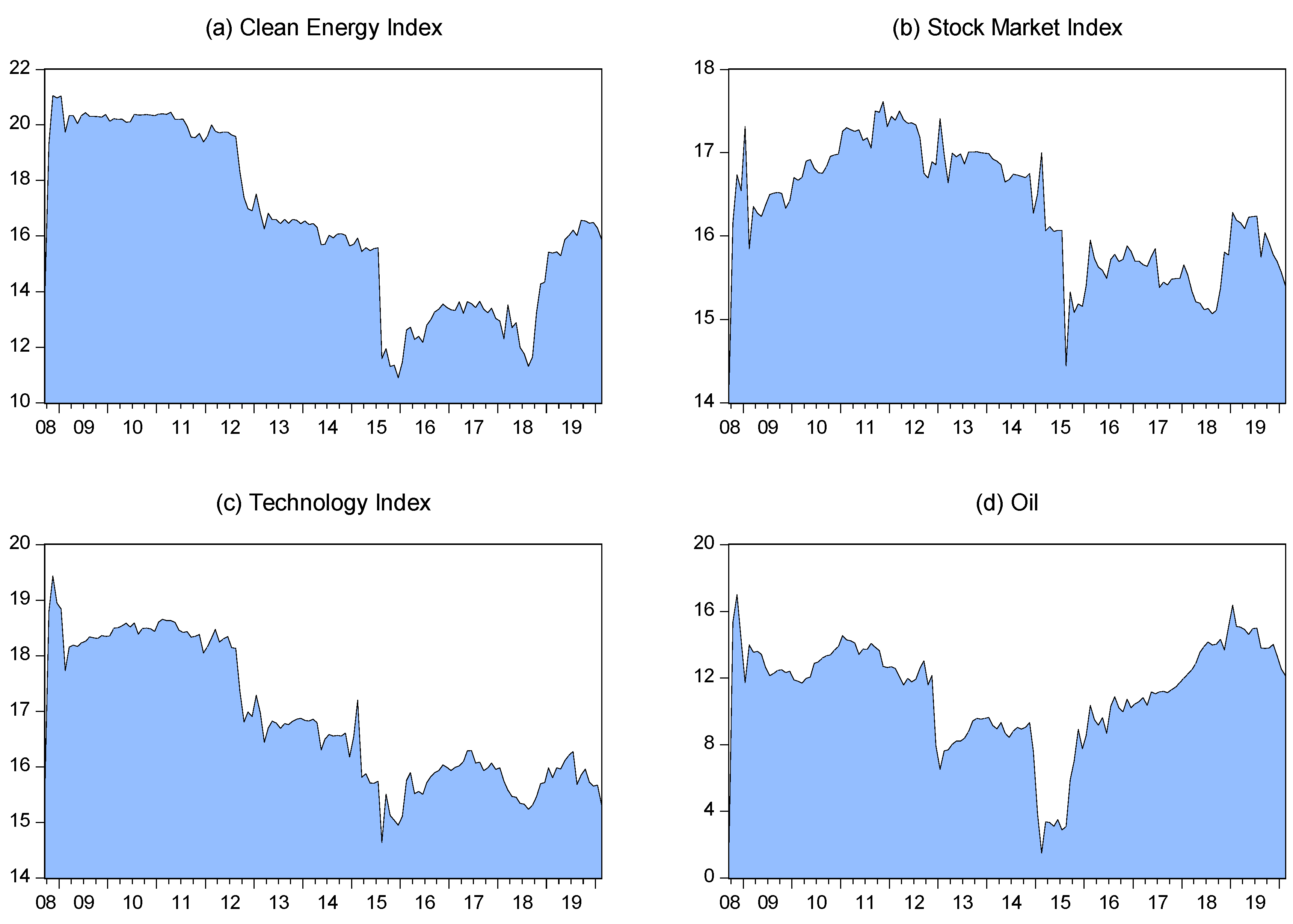
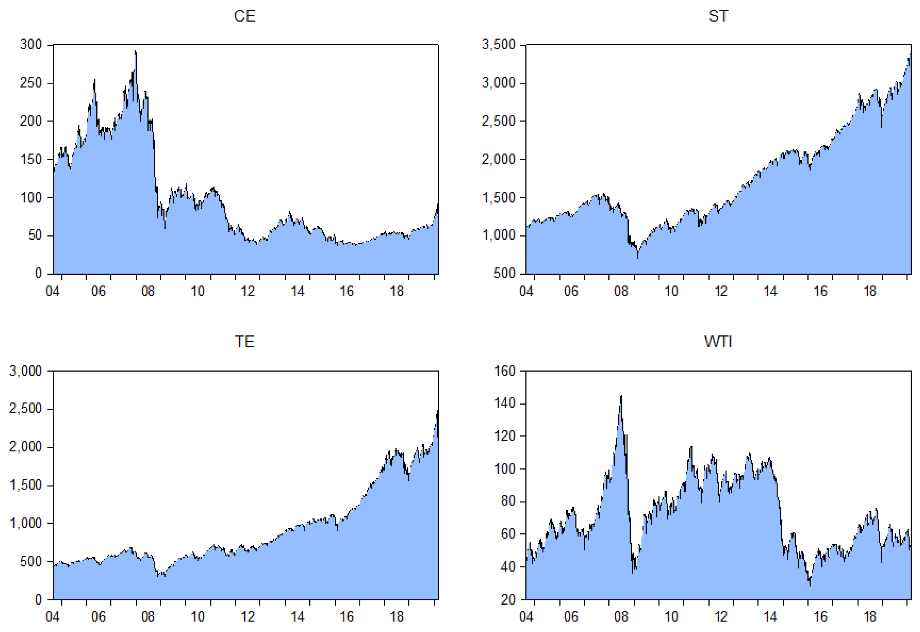
The evaluation of monthly data across the sample period is depicted in Figure 1. As shown in Figure 1, the dynamics of technology (TE) and the S&P500 (ST) index followed a similar uptrend pattern after the 2008 crisis, and they reached 2470 and 3450 points, respectively.

In contrast, the clean energy (CE) index and oil price (WTI) dropped sharply during the crisis and fluctuated until the end of our sample period. As we can see, oil prices increased until 2008 and reached their highest price (145$), but, after the economic crisis, the oil prices dramatically decreased. As a result, the clean energy index, which reached the highest record of 297 points, declined after 2008, and it fluctuated in a range of 36 to 110 points.

We can calculate the realized volatility in three steps; first, we find the percentage log return of daily data by $L{r}_{j,t}=\log \left(P_{j,t}/P_{j,t-1}\right)\times 100$, where $L{r}_{j,t}$ is the percentage log return and $P_{j,t}$ is the price level. Secondly, to find the monthly realized variance, we use $rva{r}_{j,t}={\displaystyle \sum }_{n=1}^{N}L{r}_{j,t,n}^2/N$. Finally, we calculate the realized volatility as $rvo{l}_{j,t}=\sqrt{rva{r}_{j,t}}$ [30].

Table 1. Descriptive statistics of realized volatility among the clean energy (CE), S&P 500 (ST), technology (TE), and crude oil (WTI) series.

	Clean Energy	S&P 500	Technology	WTI
Mean	0.034	0.018	0.024	0.041
Median	0.030	0.014	0.020	0.036
Maximum	0.155	0.103	0.104	0.152
Minimum	0.015	0.006	0.009	0.014
SD	0.018	0.013	0.013	0.020
Skewness	3.16	3.19	2.67	2.21
Kurtosis	17.29	17.30	13.34	9.90

provides the summary statistics for the monthly-realized volatility of all four variables. According to the mean, oil had the highest positive value, followed by clean energy, technology, and the S&P 500. Considering the risk, the standard deviation (SD) of WTI’s realized volatility is higher than that of the other indexes, and the S&P 500 records the minimum monthly volatility. The positive skewness of all four variables indicates that the volatilities are symmetric, an expected property. Furthermore, all variables have positive kurtosis (greater than 3), but the S&P 500 has the highest likelihood of experiencing extreme realized volatility.

5. Results and Discussion

Table 2. Static connectedness spillover estimates among four assets.

	CE	TE	WTI	ST	Received
CE	32.284	25.914	8.207	33.595	67.716
TE	22.558	32.700	11.162	33.580	67.300
WTI	10.555	16.352	52.570	20.524	47.430
ST	24.324	28.675	10.675	36.326	63.674
Transmitted	57.437	70.941	30.043	87.699	246.120
Including own	89.721	103.641	82.613	124.025	Spillover index
NET spillovers	−10.279	3.641	−17.387	24.025	61.530%

Note: FEVDs were computed from a VAR model with one lag selected by the Schwarz information criterion. The FEVDs were based on 10-step-ahead forecasts. All calculations were based on monthly-realized volatility data from 2004 to 2020.

presents the static connectedness estimates of the whole sample. To represent the total, directional, and net spillover, we obtained the FEVDs in a similar manner to the method of Diebold and Yilmaz [7]. The optimal lag of the VAR model was one, according to the Schwarz information criterion (SC). Hence, the values in each row indicate the spillover transmitted to other markets. The values in each column indicate the spillover received from other markets and its own market. The label “Transmitted” denotes the spillover effect from one market to another, and the “Received” shows this effect from other markets. The sum of each row, except for its own effect on the market, represents the “Received” Value.

Similarly, the sum of each column without its own effect is denoted as “Transmitted” for each market. By subtracting the Transmitted value from the Received value, we found the net spillover effect for each market. As a result, this calculation was required to understand which market was a net transmitter or net receiver. Finally, the DY time-domain spillover index (61.530%) could be calculated by summing the received (transmitted) value and dividing it by 400% (four markets $\times$ 100%).

According to Table 2, the net spillover index was 61.530% among clean energy, the stock market, technology, and oil. This shows that the connectedness of shocks can explain around 61% of FEVDs, and 39% can be considered idiosyncratic shocks. The stock market index is the significant contributor to the FEVD of the other markets with 87%, followed by technology, clean energy, and oil with 70%, 57%, and 30%, respectively. In terms of receivers, the largest one was clean energy (67%), and the lowest contributor was oil (47%). In addition, the transmission from technology to clean energy and the stock market was more than 25%, and for oil, it was around 16%. The weakest spillover effect was observed among clean energy and oil, which showed a lower connectedness among them. According to the net spillover, clean energy and oil were net receivers; however, technology and stock markets are were transmitters. The finding showed substantial connectivity among clean energy companies and technology companies, stock prices, and oil prices over the sample.

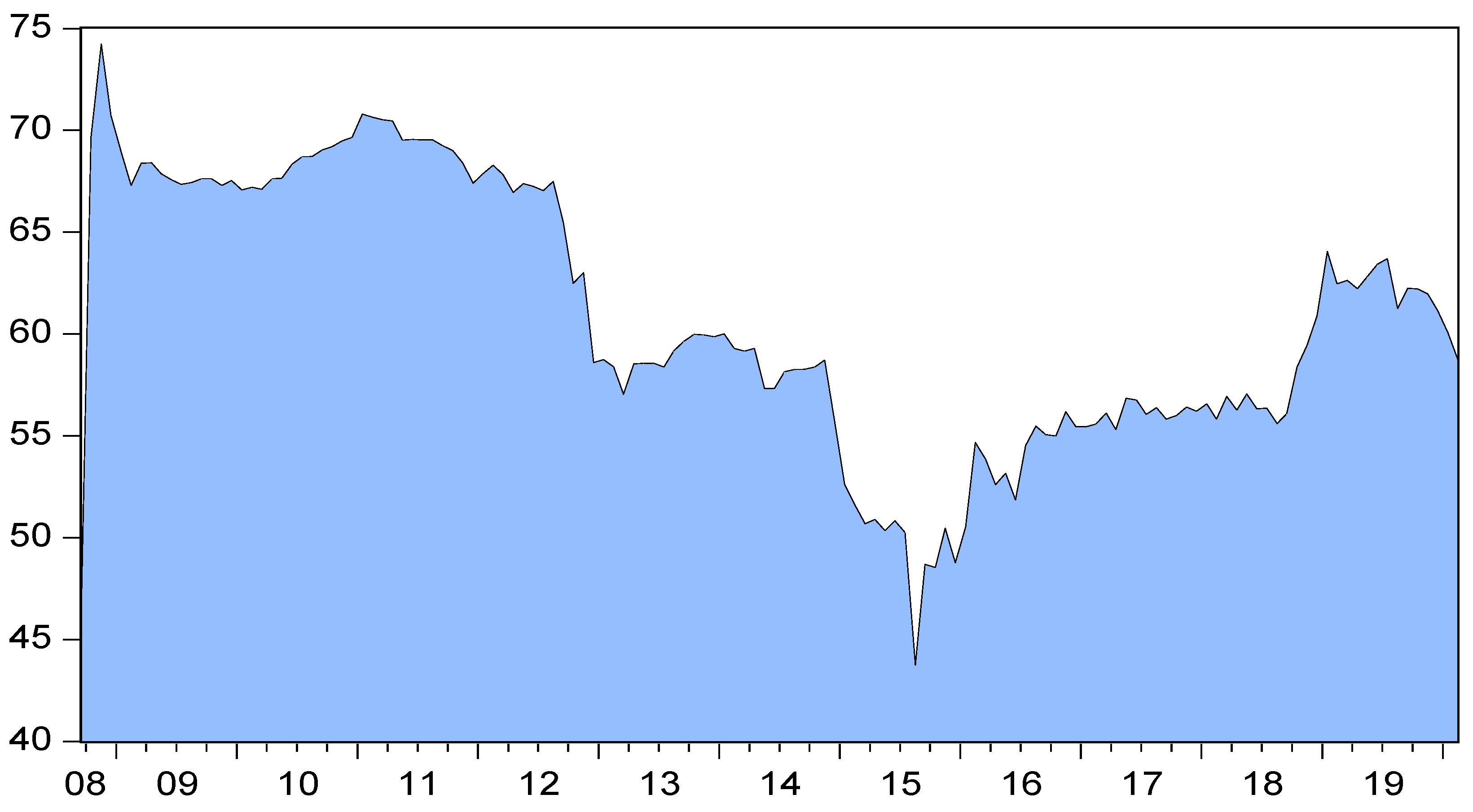
The dynamic spillover connectivity metric was then calculated using a rolling VAR model with a fixed window size of 48 months. The rolling total connectivity index is displayed in Figure 2. According to Figure 2, in the 2008 crisis (Lehman Brothers bankruptcy) and the global economic recession, the total volatility spillover index increased and reached around 74% (historic peak). After a brief transient decline at the end of 2010, the overall connectivity grew substantially during the Eurozone’s most crucial sovereign debt crisis. These results demonstrate the tremendous effect of the 2007–2008 economic meltdown and the resulting European debt crisis on spillover volatility. This confirms the common opinion that the commodity and financial market connections increase dramatically during heightened economic uncertainty. Any positive (negative) evidence is evaluated prudently in periods of confusion, thereby increasing the interconnection. In autumn 2008, the economic crisis led to an increasing spillover index, and this strengthening originated from risk aversion and uncertainty. Because of the recent international economic meltdown, market participants are becoming more aware of the market’s vulnerability to shocks. As a result, a higher-level scenario has emerged.

Consequently, the evolution of global economic and financial factors is being given more attention, which eventually has been reflected in spillovers. This finding agrees with Ahmad [18], who showed that the link between the stock prices of new energy and technology firms and crude oil prices following the international financial crisis of 2007–2008 increased dramatically. Moreover, total spillover indicators, particularly spillover volatility, decreased in 2014. This decrease in total connectivity could be attributed to the July drop in oil prices, supply considerations, such as growing US oil output, receding geopolitical concerns, and changing OPEC (Organization of the Petroleum Exporting Countries) policies, driving the initial dip in oil prices from mid-2014 to early 2015. Deteriorating demand prospects also played a role, especially between mid-2015 and early-2016. This result confirms Managi and Okimoto [20], and contrasts with Henriques and Sadorsky [10].

The volatility in China’s financial markets began in June 2015, ended in February 2016, and the spillover index increased from a low point in 2015 to a high one in 2016. Until 2019, more crises, such as those in Europe, Greece, Brazil, and Turkey, could be classified as causes of increasing spillover indexes.

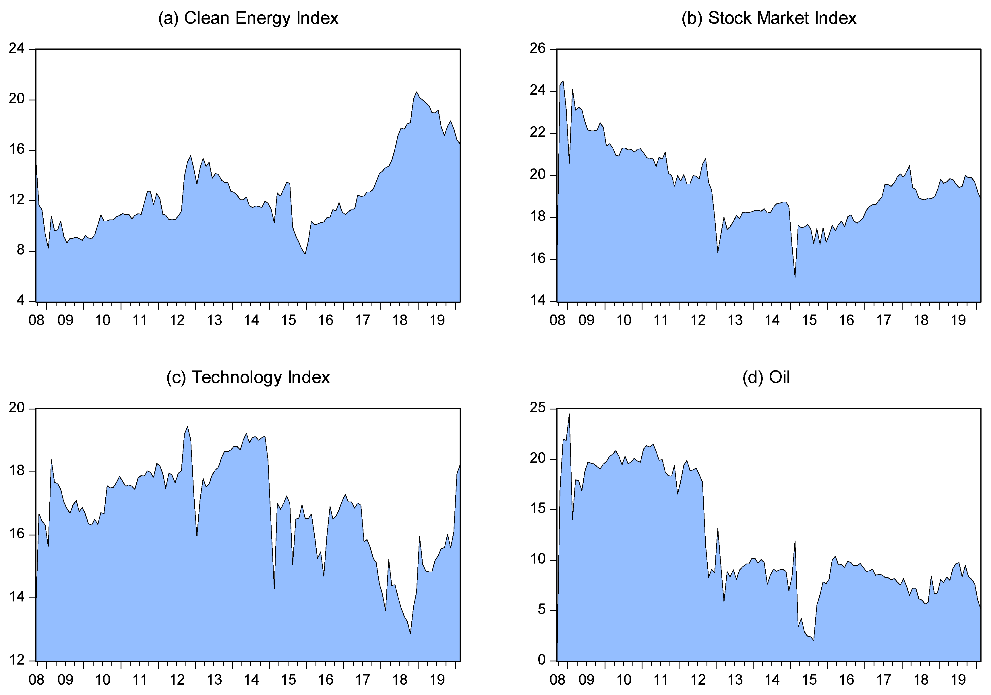
To discuss the dynamics of spillovers based on the specific asset, we used Equations (6) and (7) to estimate the directional spillovers. The directional spillovers “TO” and “FROM” are shown in Figure 3 and Figure 4, respectively. The directional volatility spillover index could be calculated by decomposing the overall spillover value. As shown in Figure 3 and Figure 4, the directional volatility spillover from other markets to clean energy rose and reached around 15%. The Lehman bankruptcy and EU debt crisis can be considered the reasons for this increase until 2012. From 2013 to 2016, there was a dramatic decline, and it could be linked to the crude oil price fall in 2014. The European stock market collapse, which can be seen in stock market Figure 3b, confirmed the sharp increase in volatility spillover since the end of 2015. The volatility spillover from another market to the stock market oscillated between 15% and 25%.

According to panel (d) of Figure 3, transmitted shocks can be classified into three groups: 2008–2012, 2012–2015, and 2015–2019, indicating the volatile period. During this period, the oil prices fluctuated because of political and economic events. However, oil transmitted shocks declined with passing time, reaching less than 5% from 24%. Figure 3c illustrates the shocks that transmitted from the technology index to other markets, and it fluctuated around 17% overall in the sample periods.

To investigate the effect of volatility spillover from other markets on clean energy, we can examine Figure 4a. As we can see, the shocks were quite large and fluctuated around 20% from 2008 to 2012. From mid-2012, the shocks received from other markets decreased, reaching less than 12%. However, from 2018 to 2020, these shocks increased by 16%. Spillover emanating from stock markets fluctuated between 14% and 18%. According to panel (c) of Figure 4, shocks started to decrease in 2008 and reached their lowest point in 2015, having a 6% range from the highest point to the lowest one. Finally, the volatility spillover in Figure 4d oscillated from 2008 to 2015 and 2015 to 2020, with the highest being 17% and the lowest being 2%.

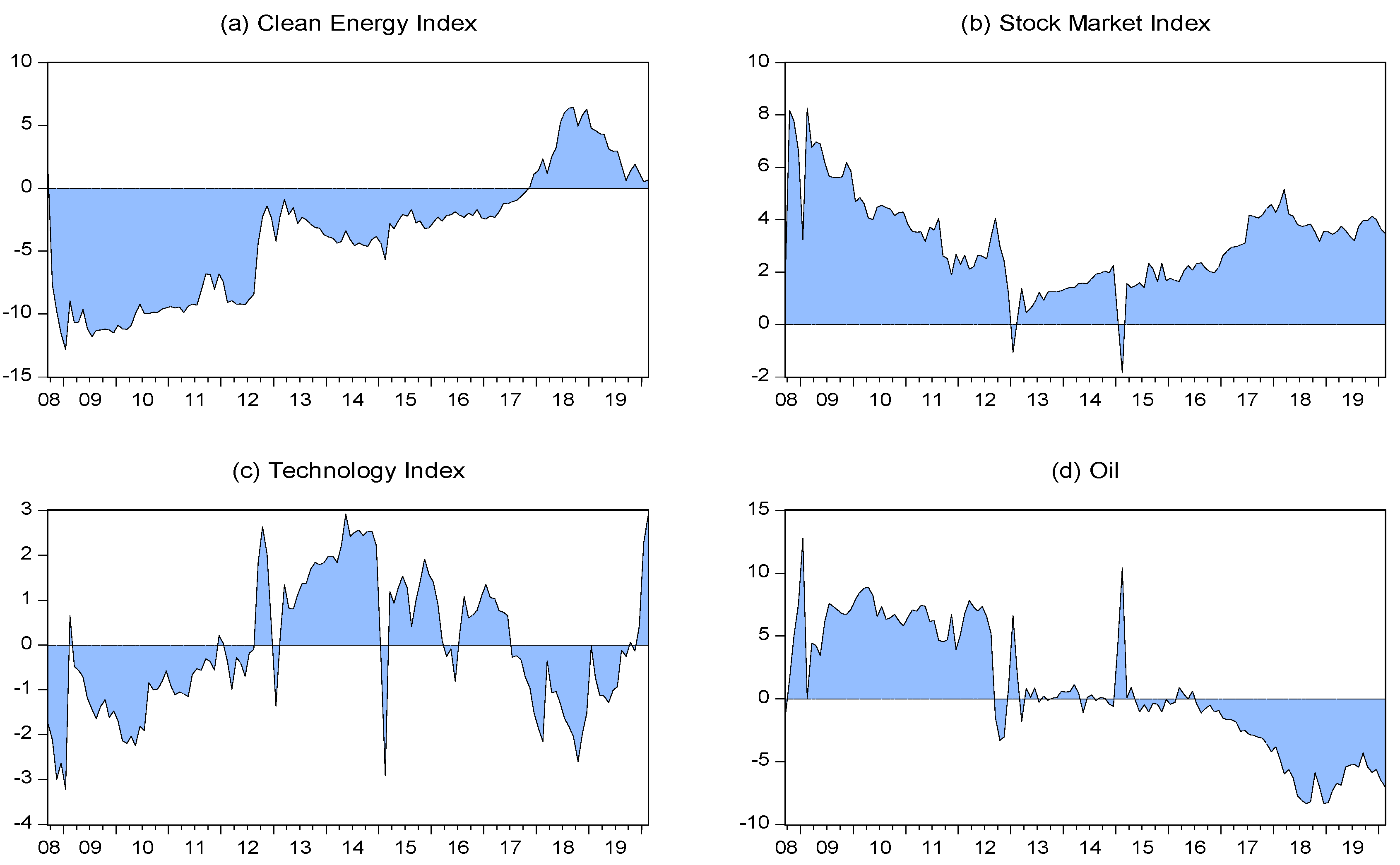
The pure time-domain method introduced by Diebold and Yilmaz [7] allows us to find net spillovers among all variables. Dynamic net spillovers can be calculated by subtracting Equation (7) from Equation (6). In this way, we can understand which market is a net transmitter (recipient) of spillovers to (from) all other variables. In addition, according to Figure 5, the negative (positive) shaded (blue) values showed the corresponding market as a net receiver (transmitter) of volatility effects from (to) other markets.

According to Figure 5, net spillovers showed a substantial difference over time; the maximum values were typically achieved at the height of the global economic meltdown, such as the Lehman Brothers’ bankruptcy, European debt, the Chinese market crash, and the oil crisis. Specifically, the clean energy stock market and oil emerged as net receivers of volatility spillovers from other markets. In contrast, technology and conventional stock markets were transmitters of volatility spillovers to all other markets. For example, as shown in Figure 5, from 2008 to 2017, clean energy was a net receiver of volatility spillovers from all other markets. In contrast, the oil market was a net transmitter of volatility spillovers to all other markets. However, after this period, the condition changed for both markets, and it showed that the dependence of other markets on the oil market started to decline.

In general, the oil and clean energy stock markets acted in the reverse direction during the whole sample period. In this way, we have evidence that clean energy and oil work in reverse. On 13 June 2014, international military intervention started against the terrorist organization the Islamic State of Iraq and Syria (ISIS), and the oil prices started to decline with the hope of peace in the Middle East. This can be considered to be a reason for the last large spike in the oil market, which acts as a net transmitter of volatility spillovers to all other markets. One of the key points is that the conventional stock market is a major net transmitter to all other markets. The role of the technology index changed between a net receiver or transmitter in the sample period, and it started as a net receiver until 2012, and from 2012–2017, it was a net transmitter. After that, it was a net receiver for two years, and in late 2019, it started to become a net transmitter to all other markets.

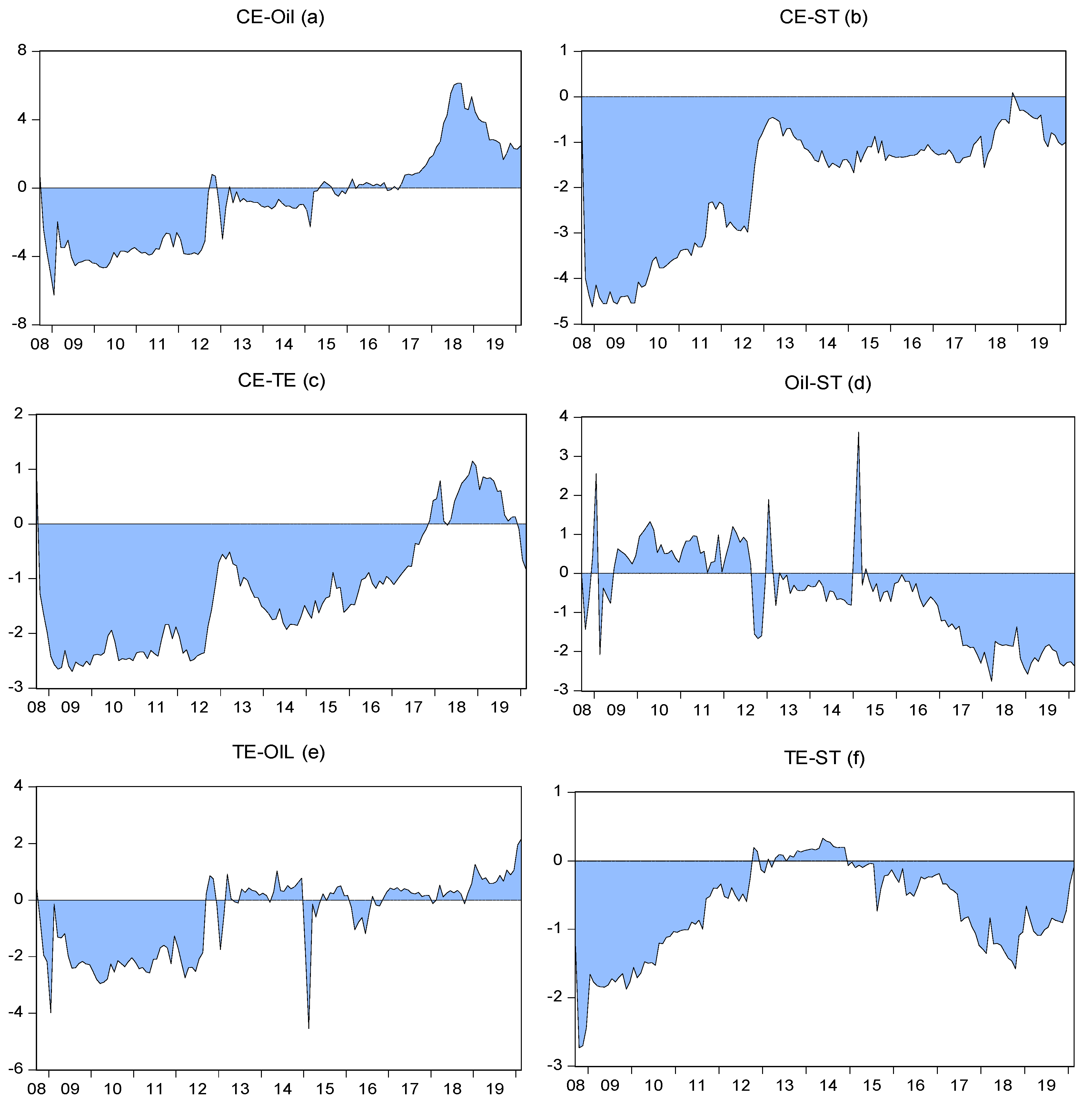
The following part focuses on the net pairwise spillover to highlight the major shocks being transmitted or received in Figure 6. Equation (9) is used to obtain the pairwise directional spillover estimates. The results confirm that clean energy was the net receiver of the shocks from technology, confirming the findings of Nasreen et al. [19]. In addition, oil transmitted the shocks to clean energy before 2014 and after the energy crisis; it was the receiver of the shocks from all of the other three assets, which contrasts with Sadorsky [15]. Moreover, this result confirms Ahmad [18], especially after the energy crisis. Comparing Figure 5a and Figure 6a, we can observe that the clean energy and oil spillovers were not significantly different.

Furthermore, we can see the same condition in Figure 5a and Figure 6c, implying that the oil and technology markets played a causal role in the clean energy market before 2014. After the oil crisis in 2014, their shocks became smaller. Concerning Figure 6b, we can see a negative net pairwise from clean energy to the conventional stock markets. We observed three large positive spikes, which could be considered significant changes in the oil market during the 2008 crisis, the Middle East and North African crises, and oil supply factors, from the last significant spike risk spillover effects, moving to conventional stock from the crude oil market, according to panel (d) of Figure 6. Furthermore, we observed that the technology index was mostly a net receiver of the conventional stock market and crude oil shocks compared to clean energy during the sample period.

6. Robustness Analysis

Dynamic financial time series interactions depend on market conditions. Asymmetric dynamics are similarly apparent compared to recessions and recovery times. Complex spillover interactions across time series data are much stronger during crisis periods (see more detail in [29,30,31,32,33]). Engle and Manganelli [34] and Kouretas and Zarangas [35] found that the characteristics of the financial time series can change significantly in terms of the supporting distribution. As a result, the dynamic interaction between the behaviors of the asset prices under consideration can be more unique in some quantiles compared to others. For example, there may be highly dynamic connections in one tail. In contrast, the connections in the other may be very low, and the DY time-domain index cannot provide reliable information on the spillovers. In other words, a simple VAR cannot show interactions between variables in non-central quantiles. The data in this paper have a non-elliptical distribution and leptokurtic characteristics (kurtosis > 3, indicating tails fatter than the normal distribution). For robustness analysis, we used the quantile vector autoregression (QVAR) model to understand the effect of larger or smaller shocks compared to mean (linear VAR) shocks. Linear VAR can investigate average shocks. Large negative and positive shocks can change the dynamics of spillover. Therefore, the QVAR can allow us to check the dynamic spillover in tails. QVAR was introduced by Cecchetti and Li [36] and followed by Xu et al. [37]. According to Chavleishvili and Manganelli [38] and Balcilar et al. [26], dynamic connections can be captured by the quantile impulse response, and they are not possible to capture by the linear VAR model. Therefore, we used the QVAR model to investigate the tail connectedness based on the approach of Cecchetti and Li [36].

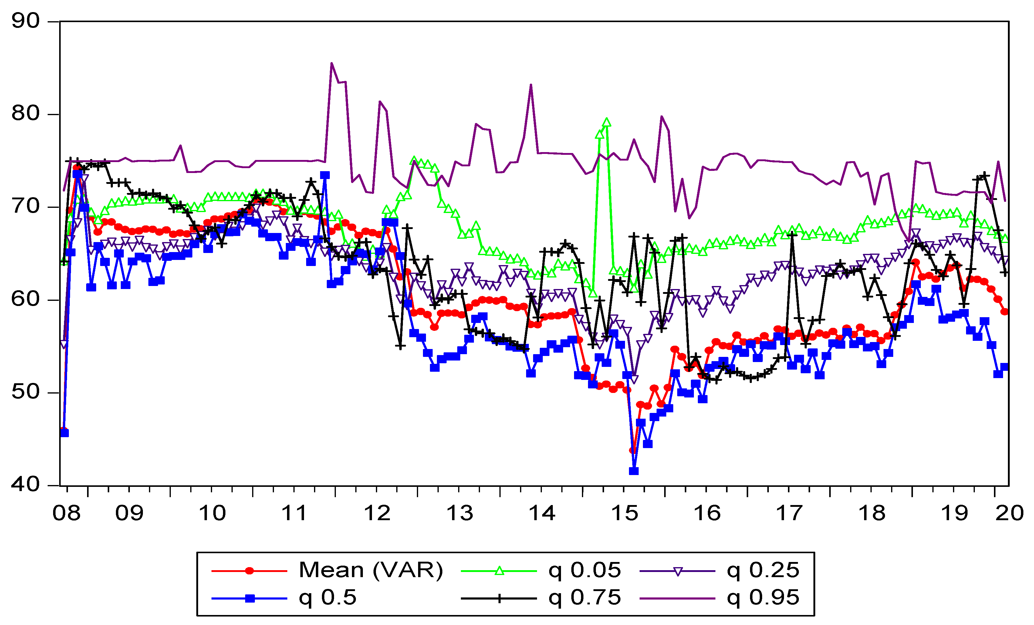
To determine whether spillovers through the renewable energy, technology, oil, and stock markets change across different quantiles, we estimated the QVAR for different quantiles. Figure 7 displays the rolling spillover indices in different quantiles (0.05, 0.25, 0.5, 0.75, and 0.95) that were extracted from the QVAR model, as well as the linear VAR as the rolling spillover index considered as the “mean.” As shown in Figure 7, the spillover indices to determine whether spillovers through renewable energy, technology, oil, and stock markets change across different quantiles, we estimated the QVAR models for different quantiles. Deviations in the mentioned quantities appeared in the range that the volatility spillovers reached the lowest level compared to the linear VAR spillovers, and the existing deviations did not reach 5%. However, we noticed that the most significant deviation was in the lower (q = 0.05) and higher (q = 0.95) quantiles than the mean results. The shortest distance between the mean and the 0.05-th and 0.95-th quantiles occurred in two different periods—the first was from the end of 2008 to 2011, and the second from 2018 to 2020. The spillover for the 0.95-th quantile was substantially more prominent for the entire period. For the 0.05-th quantile, the volatility spillover was partially greater than the VAR result in some parts of the sample. Therefore, the volatility spillover was more relevant to the large positive volatility than the average shocks. Significant negative volatility did not generate bold spillovers among the clean energy, oil, technology, and stock markets.

7. Conclusions

Over the last few decades, the massive development of the green sector has resulted in a strong desire to understand the potential of alternative energy corporations and their relationship with the oil market and economic variables. This article evaluates the dynamics of the volatility spillovers between clean energy companies, oil prices, and two notable sectors, namely the S&P 500 as a conventional stock performance index and technology index, from September 2004 until February 2020. To this end, we used the spillover index methodology based on generalized forecast error variance decomposition introduced by Diebold and Yilmaz [7]. In essence, the Diebold and Yilmaz method provides an insightful estimation of connectedness, which can be made dynamic with a rolling estimation over time. The linear VAR model results showed that the clean energy index and oil price were the net risk or volatility receivers.

In contrast, the conventional stock market and technology indices were the net transmitters of the shocks. The S&P 500 was the largest transmitter of volatility spillovers, while oil was the smallest of the four markets. In addition, during crises, such as that in 2008, the total connectedness rose sharply. Based on the results, there is a strong bidirectional spillover between these markets. Balcilar et al. [26] estimated dynamic spillovers between gold, oil, and the S&P 500. They concluded that, in financial and non-financial economic instability periods, the importance of oil and gold as a safe haven has shifted throughout time. According to our results, the role of oil prices in the energy market will change with the stock markets, and energy will be compensated with clean energy in the following decades. Additionally, we can conclude that the S&P 500 and the technology markets play a crucial role in the clean energy market according to the net pairwise spillover results.

The results of our study contradict Sadorsky’s [15] conclusion that oil is a good hedge for renewable energy stocks. The findings suggest that oil price fluctuations are not the most important factor affecting the profitability of renewable energy and technology enterprises. These corporations have the influence to alter their course in response to a business environment that is less reliant on the oil market. Investors may assume that technological breakthroughs and inventions are critical to the profitability of renewable energy and technology firms, as well as their stock values. The oil market could lose its significance because of the domination of clean energy firms and the expansion of energy-efficient production processes. The evidence of a close link between clean energy and technology enterprises implies that policymakers should recognize that the clean energy market’s future depends on new technology innovation and uptake. As a result, clean energy companies must have an energy strategy to compete with technological product innovation. This study’s empirical findings are useful for investors, financial managers, and portfolio managers dealing with market uncertainty during oil price shocks. The insights can also help technology businesses identify hedging and arbitrage opportunities. When dealing with oil and stock portfolios, investors must also consider the duration and nature of oil price shocks.

The results of this paper may have significant implications for investment decisions and risk assessment from different financial perspectives. Moreover, policymakers should also be aware that, if oil prices remain low, alternative energy production industries do not need specific policies to reduce their susceptibility to crude oil price shocks and simplify the energy sector’s shift into a sustainable one. Instead, policies that promote clean energy development should be ideally geared towards improving investment and clean energy innovations. The presence of stronger spillover in the tails, on the other hand, suggested vulnerability to the effects of extreme events, such as wars and financial crises. The spillover among the markets was particularly high in the upper tail, with values usually around 75% at the 0.95-th. In the lower tail, the spillover was also higher than at normal times, fluctuating around 65% to 70% at the 0.05-th quantile. Therefore, extreme events may generate quite significant spillover risks. Wars and financial crises usually cause large rises in oil prices and crashes in stock prices. Thus, policymakers should consider the fragility of markets to oil price and stock market spillover risks during extreme event periods. Finally, in the empirical economics literature, there are various methods for modeling nonlinear relationships between economic and financial variables. The vector threshold autoregressive, vector smooth transition autoregressive, and vector- Markov switching autoregressive models are the most used parametric nonlinear VAR models. The results of this study can be further extended with these nonlinear models with different interconnected assets in local or international marketplaces.