Numerical Investigation of the Application of Miller Cycle and Low-Carbon Fuels to Increase Diesel Engine Efficiency and Reduce Emissions

Abstract

In this paper, validated simulations using Ricardo WAVE have been performed to investigate the effect of the Miller cycle and low-carbon fuels on the performance (power, torque, BTE and BSFC) and emissions of a diesel engine. The results show that the increased Miller cycle effect (larger deviation of the advanced or retarded intake valve closing from the standard intake valve closing time) will decrease NO_x, CO and HC emissions, and slightly improve brake thermal efficiency (BTE) and brake specific fuel consumption (BSFC) with slight loss in engine performance and increase in soot emissions. An engine running B0 (diesel with 0% Biodiesel in the blend) with a −18% Miller cycle effect has a reduction in NO_x of 9% and CO of 4.3% with a decrease of 1.6% in power at the rated engine speed. Using low carbon fuels drastically reduces emissions with reduced BTE and increased BSFC. When used in conjunction, the Miller cycle and low-carbon fuels have an improved effect on both performance and emissions. The optimal results demonstrate that using B60 (60% Biodiesel in the blend) and a −8% Miller effect contributes to a 1.5% improvement in power, 1.2% in BTE, 13.3% in NO_x, 38.5% in CO, 8.9% in HC, and 33.0% in soot at a cost of 6.0% increase in BSFC. The results show that it is an easy way to reduce NO_x, CO, HC and soot emissions and increase the BTE of the engine by combining Miller cycle and low-carbon fuels.

1. Introduction

DIESEL engines are used extensively worldwide in vehicular and static applications. Nitrogen Oxide (NO_x) and other emissions from diesel engines are significant, and often above safe levels in built-up areas. In the UK, diesel consumption grew from 11 million tonnes of oil equivalent (MTOE) in 1990 to 27 MTOE in 2017, and 21% of the UK’s greenhouse gas emissions were from road transport in 2017 [1]. Large vehicles such as lorries account for 76% of excess NO_x emissions [2]. The issues arising from NO_x have led to strict legislation, with limits for NO_x under EU standards Euro 5 and Euro 6 of 0.18 g/km and 0.08 g/km [3]. This shows a need to find adaptations for diesel engines to counter these emissions problems [4].

The Atkinson cycle was first developed in 1882 and was achieved by mechanical methods [5]. This involved altering the effective compression stroke of the engine by either early intake (EIVC) or late intake (LIVC) valve closing [6]. In both EIVC and LIVC, the compression stroke is effectively shorter than the expansion stroke, which improves the brake thermal efficiency (BTE) of the overall cycle [6]. However, since some fuel and air escape before combustion, the power output and brake mean effective pressure (BMEP) is decreased [7]. Ralph Miller adapted this cycle to include a turbocharger or supercharger at the cylinder inlet [8,9]. This pushes air into the engine cylinder, leaving it at a higher pressure [9]. This may reduce brake specific fuel consumption (BSFC) [10] and mitigate the power loss often found with the Atkinson cycle [11]. Once the piston is beyond bottom dead centre (BDC), the boosted charge compensates for the open inlet valve ensuring similar air/fuel charge to a non-Miller cycle unit. Powell et al. [12] validated the Miller cycle theory using a Ricardo WAVE model and experimentation, and found the fuel consumption was reduced by 5.6% when using the LIVC. Lin and Hou [13] analysed an air-standard Miller cycle and found engine efficiency improved over the Otto cycle. In addition to improving engine efficiency, the Miller cycle can be used to reduce NO_x emissions [14,15,16]. Other methods such as after treatment can reduce NO_x in exhaust gases, but are expensive [17]. The shorter compression stroke of the Miller cycle means a lower compression ratio, with consequent reduction in cylinder pressure and temperature. Lower temperature in cylinder will produce less NO_x, since NO_x forms rapidly at high temperatures, especially above 1600 K [18]. This reduction in NO_x emissions has been shown experimentally [14,19,20,21]. Test results showed a decrease in NO_x emissions of 60% and in soot of 25% [21]. In another experiment, the torque, power, BTE and BSFC were improved at high engine speeds and worsened at low speeds due to the charge loss and the drop in volumetric efficiency, but NO_x emissions reduced by 14% [20]. The difference between standard cycle and Miller cycle is illustrated in Figure 1 for diesel engine, where the cycle 0–1a–1′a–2a–3a–3′a–4a–1′a–1a–0 is the Miller cycle and the 0–1–2–3–3′–4–1–0 is the standard cycle.

Low-carbon fuels have a lesser impact on the environment than fossil-fuels [22], and can be split into three categories [23]: first-generation biofuels; advanced or second-generation biofuels; renewable fuels of nonbiological origin. Using low-carbon fuels may affect the efficiency and emissions of a diesel engine [24,25]. Experiments showed increase in BSFC of 2.1%, 1.5%, 3.5% and 9.6% for B10, B20, B50 and B100, respectively [24], which was attributed to the lower calorific value of biodiesel [26]. Meanwhile, the BTE is also impacted by using biodiesel. At 10% load the BTE for B100 was 10.2% lower than pure diesel, but was 5.1% higher at 100% load, with a crossover point at 50% load. This behaviour could be attributed to several factors: at high load, fuel injection pressure was at its highest, so the effect of the viscosity of biodiesel was negligible [26]; B100 contains oxygen, which may contribute to a more complete combustion [27], thus increasing BTE; at lower loads, the viscosity of biodiesel was more influential and may reduce BTE, and the oxygen content of the fuel may make the mixture lean, which decreased BTE. Moreover, it is claimed that as biodiesel concentrations increases, combustion temperature and NO_x emissions increase [28,29]. Mueller et al. [30] stated that the increase in combustion temperature cannot quantitatively be related to a single parameter, but instead is due to several coupled mechanisms which change under different conditions such as fuel or combustion characteristics. Kegl [31] found that in a B100 mixture, the higher injection pressure and oxygen content reduced soot and CO emissions. Higher NO_x emissions also arose from the advanced injection process with earlier and prolonged high temperatures at combustion commencement. Others found that higher proportion of biodiesels lower the exhaust temperature [24,32]. It was found that the exhaust gas temperature was linked to the compression ratio. At low ratios of 18, the exhaust gas temperature for biodiesel was higher than that of diesel, but as the ratio increases the exhaust gas temperature of biodiesel is lower than that of diesel [32]. It is also theorised that the reduction in exhaust temperature is due to the lower calorific value of biodiesel reducing the total released energy and therefore the peak temperature [24,26,32].

It is found that existing studies have not accounted for the effect of the combination of the Miller cycle with low carbon fuels on the performance of diesel engine, particularly in maximising efficiency and minimising NO_x and other emissions. Consequently, this study will investigate the influence of combining the Miller cycle and low carbon fuels on diesel engine performance and emissions. The following objectives will be covered:

• Develop the numerical model of a diesel engine and validate it using verified data.
• Obtain the engine performance and pollutant emissions of standard diesel fuel with various Miller cycle effects.
• Obtain the engine performance and pollutant emissions of different low carbon fuel-diesel blends without Miller cycle.
• Combine the low carbon fuel blends and Miller cycle effects, and find the optimal low carbon fuel fraction and Miller cycle effect.

2. Method

In this paper, biodiesel fatty acid methyl esters (FAME) are selected as the low carbon fuel. It is blended with diesel fuel with various fractions, namely B0 (standard diesel fuel), B7 (7% volume fraction for biodiesel), B20, B40, B60, B80, and B100. The properties of FAME and its blends with standard diesel fuel are listed in

Table 1. Comparison of heating value of fuel types.

Fuel Type	Energy Content (MJ/kg)	Density at 20 °C (kg/L)	Viscosity at 20 °C (mm2/s)	Cetane Number
B0	43.1	0.83	5.0	50
B7	42.58	0.834	5.175	50.42
B20	41.8	0.84	5.5	51.2
B40	40.6	0.85	6	52.4
B60	39.4	0.86	6.5	53.6
B80	38.2	0.87	7.0	54.8
B100	37.1	0.88	7.5	56

. Numerical modelling is used to implement the low carbon fuel and the Miller cycle configurations. Ricardo WAVE was chosen as the modelling software as a state-of-the-art gas dynamics simulation tool used ubiquitously within the automotive sector. The numerical model is well established and validated against data from database [33].

2.1. Theories

In the model, the details of the flow is obtained by solving quasi-one-dimensional compressible flow equations that govern the conservation of mass, momentum and energy [33,34]. A staggered mesh system is used with the boundaries between volumes to solve the equations of momentum, mass and energy for each volume. In explicit conservative form, the equations can be written as:

$$mass=\frac{dm}{dt}=\mathsf{\Sigma } \dot{m}$$

(1)

$$momentum=\frac{dmu}{dt}=-A\frac{dp}{dx}+\mathsf{\Sigma }\dot{m}u-sources$$

(2)

$$energy=\frac{d{e}_T}{dt}=\mathsf{\Sigma }mh+sources$$

(3)

The general combustion equation solved in the model is:

A(uN₂ + vO₂ + wCO₂ + xH₂O) + B(C_cH_hO_oN_n)
aCO + bCO₂ + cH + dH₂ + eH₂O + fN₂ + gNO + hO + iO₂ + jOH + kN

(4)

where, A is the mass fraction of ‘Burned Air’, B is the mass fraction of ‘Burned Fuel’; and a, b, …, k are the coefficients of the combustion products. The sum of $A$ and $B$ is the total mass fraction of combustion products, and the ratio between them gives the relative quantities of the species. Normally, the entire fuel mass is burned with product mass fractions that sum to 1; the values of the coefficients a to k are uniquely linked to the equilibrium equation [33,34].

In terms of combustion, the Diesel Wiebe combustion model is used to obtain the rate of fuel mass burned, which includes the premixed combustion, diffusion combustion and slow late combustion (tail burning) in the engine cylinder [33]. The burned fuel mass fraction W based on the crank angle can be calculated from the following equation.

$$W=p_f\left\{1-{\left[1-{\left(0.75\tau \right)}^2\right]}^{5000}\right\}+d_f\left\{1-{\left[1-{\left(c{d}_3\tau \right)}^{1.75}\right]}^{5000}\right\}+t_f\left\{1-{\left[1-{\left(c{t}_3\tau \right)}^{2.5}\right]}^{5000}\right\}$$

(5)

where $p_f$, $d_f$ and $t_f$ are the mass fractions of the premixed, diffusion and tail combustion, respectively, whilst $\tau$ is the burn duration term determined by Equation (6).

$$\tau =\frac{\theta -{\theta }_b}{125{\left(\frac{RPM}{BRPM}\right)}^{0.3}}$$

(6)

$\theta$ and ${\theta }_b$ here refer to the crank angle and the crank angle at the start of combustion, respectively, whilst $RPM$ and $BRPM$ are the engine speed and reference speed. The mass fraction of the premixed combustion can be either user-input or obtained from the ignition delay model.

For emissions, the NO_x emissions are predicted using the Zeldovich mechanism (Equations (7) and (8)) and the Prompt mechanism (Equations (10)–(12)) [35]. The overall burned zone is treated as an open, stratified system in which further NO_x formation takes place depending on the temperature, pressure, and equivalence ratio.

$$O+N_2\rightleftharpoons N+NO$$

(7)

$$N+O_2\rightleftharpoons O+NO$$

(8)

$$CH+N_2\rightleftharpoons \mathrm{HC}N+N$$

(9)

$$N+O_2\rightleftharpoons NO+O$$

(10)

$$HCN+\mathrm{OH}\rightleftharpoons H_{2}O+CN$$

(11)

$$CH+O_2\rightleftharpoons NO+CO$$

(12)

CO is calculated based on the following model dependent on pressure (P), concentrations of substances including [CO₂], [O₂], [OH] and [H], and equilibrium constants ($K_{pW}$ and $K_{pN}$) suggested by Newhall [36].

$$\frac{\left[CO\right]}{\left[C{O}_2\right]}=max\left(\frac{1}{\sqrt{K_{pW}P\left[O_2\right]}},\frac{\left[H\right]}{\sqrt{K_{pN}P\left[OH\right]}}\right)$$

(13)

HC model assumes that the fuel trapped within the injector sac and hole volume is the major source of unburned HC, and the emitted HC is proportional to the injector sac volume. The typical injector sac volume is in a range of 0.3 to 1 mm³, and about 0.2 of sac volume fuel is converted to HC [33].

Soot model accounts for the soot formation and oxidation rates. The soot formation rate is based on Khan–Hiroyasu–Belardini formulation, and the soot oxidation rate is based on the Nagle and Strickland–Constable model [33]. The soot formation rate $\frac{d{M}_{sf}}{dt}$ is calculated by the equation:

$$\frac{d{M}_{sf}}{dt}=k_f{M}_{fv}$$

(14)

where $M_{fv}$ is the fuel vapor mass, and $k_f$ is a coefficient dependent on the fuel properties and temperature. The soot oxidation rate $\frac{d{M}_{so}}{dt}$ is calculated by

$$\frac{d{M}_{so}}{dt}=\frac{M_c}{{\rho }_s{D}_s}{M}_s{R}_{rov}$$

(15)

where $M_s$ is the net soot mass, $M_c$ is the carbon molecular weight, and $R_{rov}$ is the reaction rate dependent on temperature. The soot density ${\rho }_s$ and soot mean diameter $D_s$ are constants.

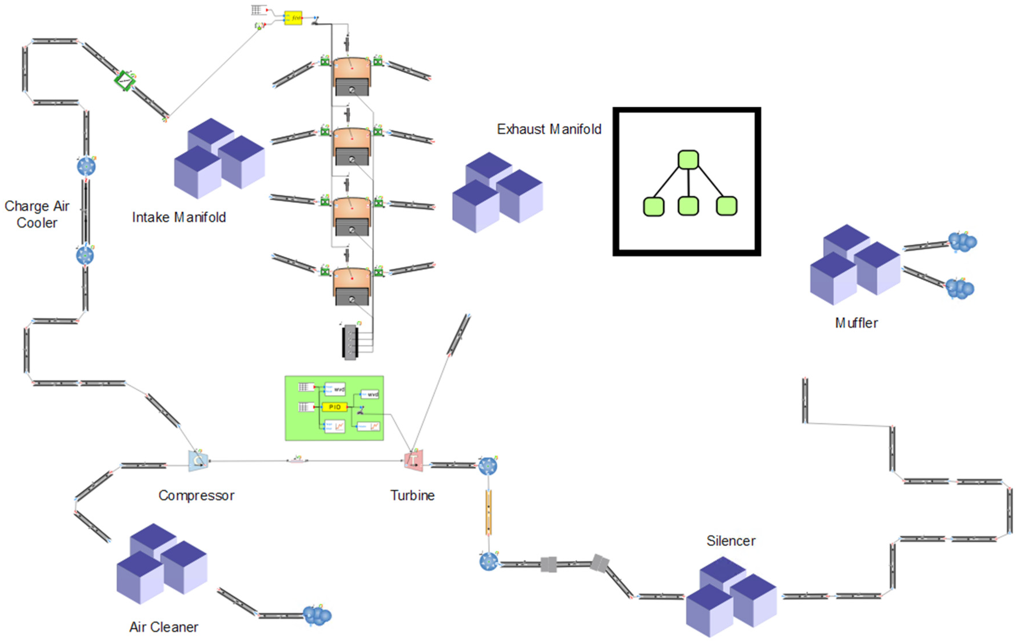
2.2. Model Set up and Procedure

A Volkswagen 1.9L variable-geometry turbocharger (VGT) TDI PD diesel engine is selected as the test engine, which is used in a wide range of midsized cars. The engine specification is shown in

Table 2. Specification of the test engine.

Parameter	Test Engine
Displacement (L)	1.9
Bore (mm)	79.5
Stroke (mm)	95.5
No. Cylinders	4
No. Valves per cylinder	2
Max Power (kW)	96 at 4000 rpm
Max Torque (Nm)	310 at 1900 rpm
Turbocharger Type	VGT

.

The numerical model of the selected 4-cylinder engine is set up according to its specifications, as shown in Figure 2. The model is validated and then used to investigate the engine performance under the proposed conditions, i.e., the designed combined Miller cycles and a number of different low-carbon fuels.

The procedure of setting up the model is in the following steps:

(1)

Generate engine components and link them together to form a basic engine model in the WAVE;

(2)

Define geometry and boundary conditions of the engine, such as bore, stroke, intake temperature, etc., and select fuels;

(3)

Validate the model using data from the engine manufacturer;

(4)

The validated model is then used to do intensive simulations of the engine performance under the normal cycle of diesel engine and the selected Miller cycles, to find out the optimal results.

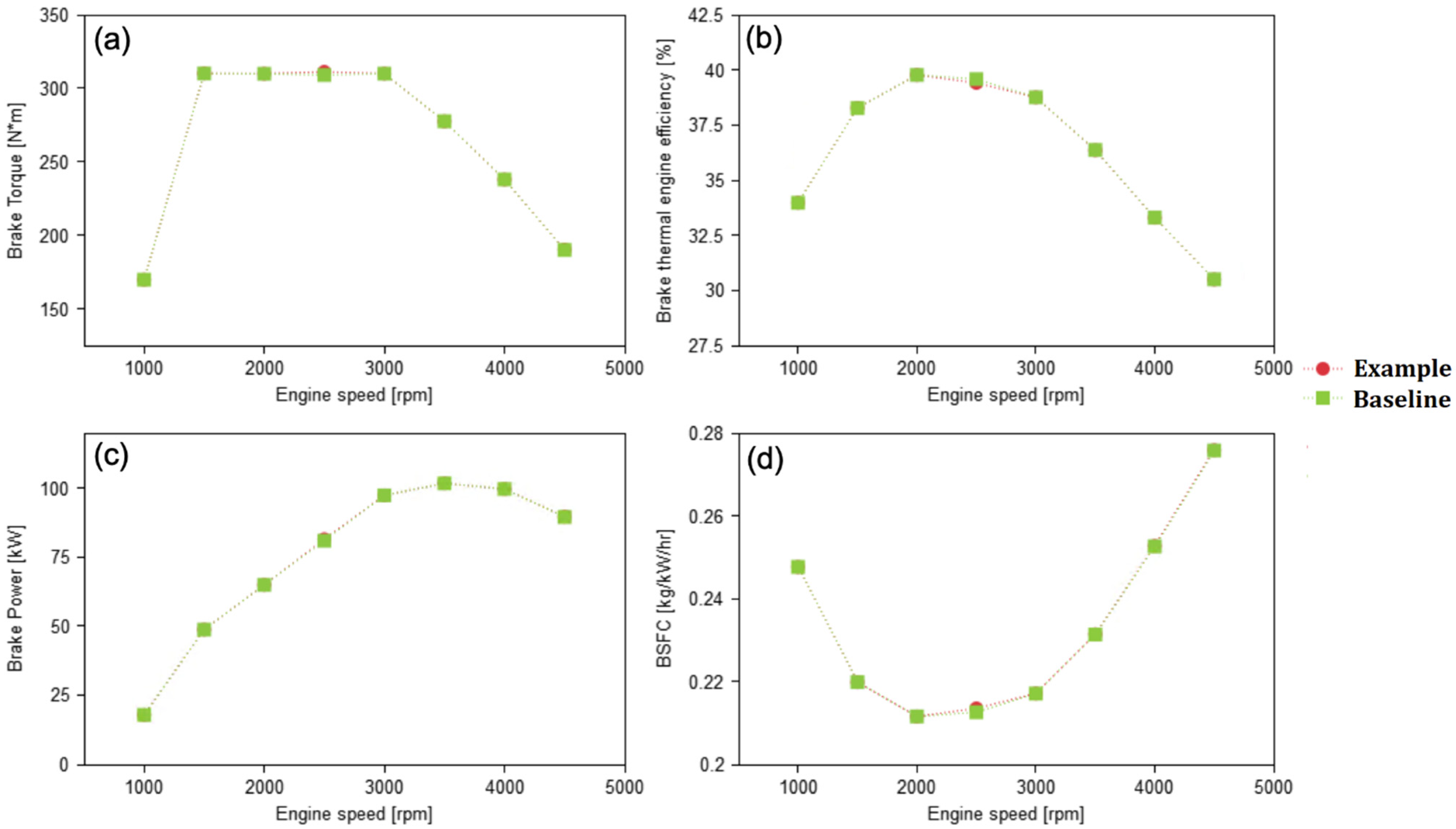
2.3. Model Validation

The numerical model is set up based on the specifications of the test engine to run the fuel B0 with no Miller cycle effect, which is named as the baseline model. The baseline model is run at the speeds from 1000 rpm to 4500 rpm at full load. Richard Wave database provides an example model for the same engine at the same conditions, and its results have been verified by experimental data [34]. Therefore, the data from the example model is used to validate the baseline model. The results are shown in Figure 3 and Figure 4, where the green dots/line are the performance of the baseline model, whilst the red dots/line are that of the example model. It is clear that the models have close results in performance and emissions with the largest difference of 0.686% at 2500 rpm. It indicates that the model is well validated, and thus can be used for further investigations.

2.4. Computational Simulations Planned

Using the validated model, totally 77 cases of combined 11 Miller cycles with the 7 low-carbon fuel-diesel blends are carried out under different conditions: (1) the original engine; (2) 5 cases of early intake valve closing (EIVC) Miller cycle; (3) 5 cases of late intake valve closing (LIVC) Miller cycle; and (4) low-carbon fuel-diesel blends with 7 fractions shown in Table 1. The fuels are the mixture of biodiesel with diesel, where ‘B’ is ‘biodiesel’, the number of ‘0, 7, 20, 40, 60, 80 and 100 represents the mass fraction of the biodiesel, e.g., B20 is a fuel with 20% of biodiesel and 80% of diesel in it. The test conditions of Miller cycles are listed in

Table 3. The test conditions of Miller cycles.

Miller Cycle Percentage (%)	Change in Crank Angle (°)	New Open Duration (°)
−25%	−64.5	193.5
−20%	−51.6	206.4
−15%	−38.7	219.3
−10%	−25.8	232.2
−5%	−12.9	245.1
0	0.0	258.0
5%	12.9	270.9
10%	25.8	283.8
15%	28.7	296.7
20%	51.6	309.6
25%	64.5	322.5

. The percentage of Miller cycle is calculated by comparison to the original intake valve opening duration (258°). For example, the intake valve opening durations of the EIVC cases are smaller/shorter than that of the original ones, and the changes in crank angle is negative, e.g., −5% Miller cycle Percentage, the intake valve opening duration is 245.1°, which is 5% less than that of the original one (258°). Similarly, the intake valve opening durations of the LIVC cases are longer than that of the original ones, e.g., 5% Miller cycle percentage, the intake valve opening duration is 270.9°, which is 5% longer than 258°.

The range tested was between 1000–4500 rpm, which is the normal operating range of the engine, giving 8 data points for each case. The engine performance parameters such as brake power, brake torque, brake thermal efficiency (BTE), brake specific fuel consumption (BSFC) were obtained. The major emissions including nitrogen oxide (NO_x) and soot were collected in each case, and other low-level emissions such as carbon monoxide (CO) and unburned hydrocarbon (HC) were also accounted.

3. Results and Discussion

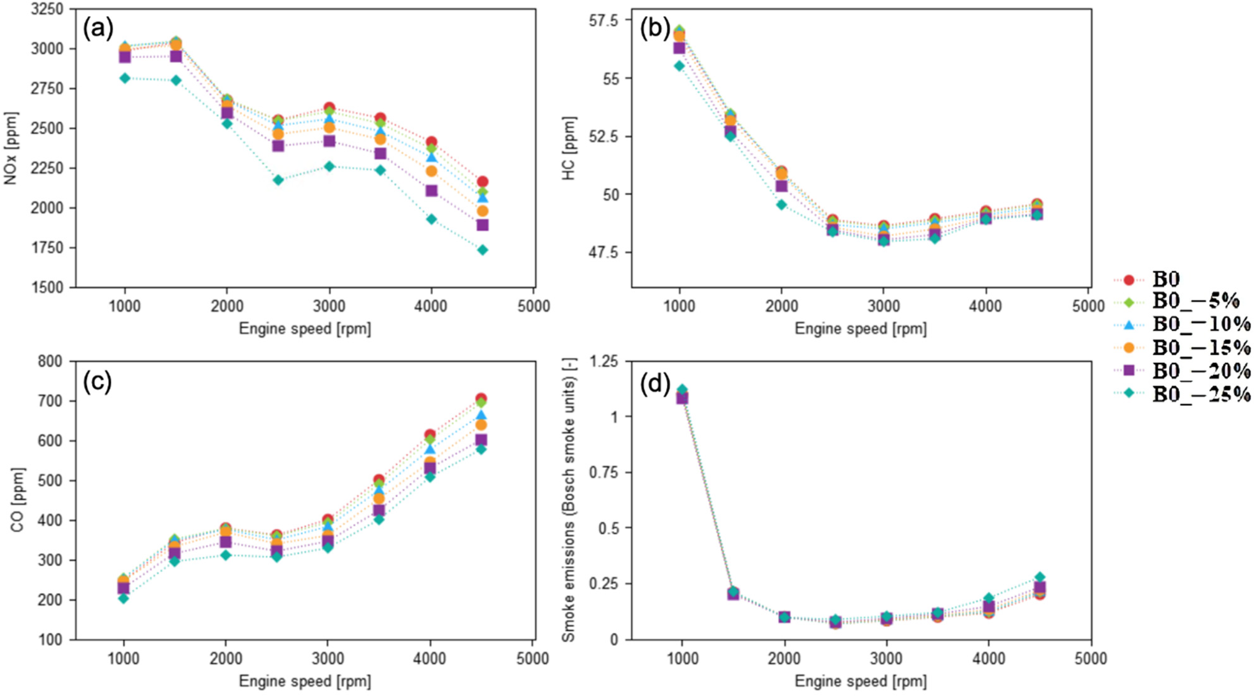
3.1. Effect of Miller Cycle with B0 Fuel

Figure 5 shows the effect of the 5 LIVC Miller cycles (plus the baseline model being the original diesel engine) using B0 fuel. In all figures, each name in the legend shows the fuel used firstly and then the condition in Miller cycle. For example, the ‘B60_−10%’ means that B60 fuel is used with a negative (EIVC) Miller cycle effect of 10%.

Figure 5a–d show the effects of the different LIVC Miller cycles on the engine performance, i.e., brake torque (BT), brake thermal engine efficiency (BTE), break power (BP) and brake specific fuel consumption (BSFC), respectively. At the engine speeds of 3000 rpm and above, there is a slight decrease in BP, BT and BTE relative to the baseline in each case. The figures also demonstrate that at lower engine speeds, the increasing LIVC Miller effect has a drastic negative effect on engine performance. For example, in the case of 25% LIVC Miller cycle at 1000 and 1500 rpm, the engine torque is less than half of that in the baseline, because the turbocharger is unable to compensate for the reduced valve opening durations at low engine speeds.

As the Miller effect increases, the engine performance decreases, as shown in Figure 5. For example, the 5% Miller curve (the green ‘squares’ and the green line in the figure) matches the baseline engine at nearly every point, only dropping in the lower speed range of 1000–1500 rpm, whereas a noticeable drop in torque occurs to the 20% Miller curve (the purple ‘dots’ and the purple line) at the higher engine speed of 2500 rpm. The peak power of the baseline engine occurs at 3500 rpm, but the Miller cycle has little effect at the same speed even with the stronger Miller cycles, which causes the engine performance decrease at lower speeds.

The reason for the performance decrease in the LIVC Miller cycles is that part of the intake air and some injected fuel (between the starting of fuel injection to the point of intake valve closed) is pushed out of the cylinder when the intake valve closes later, which is wasted and thus reduce power, torque, BTE and increase BSFC.

Figure 6 shows the effects of the different LIVC Miller cycles on emissions. The Miller cycle shows a significant reduction in NO_x and CO emissions, especially at lower engine speeds, and a smaller but still noticeable improvement at engine speeds above 3000 rpm. The correlation between the extent of Miller effect and the improvement in emissions is demonstrated that the stronger the Miller cycle effect, the lower the NO_x and CO emissions. The peak decrease in NO_x emissions is with 25% Miller cycle at 1500 rpm where there is a decrease in NO_x of 26%.

The HC emissions also decrease as the Miller cycle effect is enhanced, but the extent of the decrease is than that in NO_x or CO, which indicate a weaker link between Miller cycle effect and HC emissions. The HC emissions decreased at all engine speeds, with a maximum decrease of 1.7% at 2000 rpm.

Soot emissions are sensitive to the Miller cycle effect and increased by stronger Miller cycle. Soot emissions reach the highest value at lower engine speeds when running at LIVC, with a peak increase of 152.7% at 1500 rpm and 4.1% at 3500 rpm for 25% Miller effect. The reason for the soot increase in the LIVC Miller cycles is that, as mentioned above, part of the intake air and some injected fuel is pushed out of the cylinder when the intake valve closed later. Consequently, it is not burnt under the low temperature in the exhaust pipe, but decompose to carbon particles or other hydrocarbon particulates and emit in the form of soot.

Figure 7 shows the effect on different degrees of early intake valve closing (EIVC) Miller cycle using B0. Apart from the extreme value at −25% Miller, much less severe impact on performance is observed compared with that of LIVC Miller cycle in Figure 5. Up to a −20% Miller effect, no comparable negative effect is found on engine performance, apart from a small decrease in power and torque at 4000 rpm. At the rated speed, there is almost no loss in torque or power, as shown in

Table 4. The effect of the Miller cycle including both Eivc and Livc on the performance and emissions of a pure diesel engine at the rated speed, 3500 rpm (differences in % to the baseline without Miller cycle).

Miller Cycle (%)	Torque (%)	Power (%)	BTE (%)	BSFC (%)	NOx (%)	CO (%)	HC (%)	Soot (%)
−25	−5.32	−5.32	−0.87	0.88	−12.80	−19.97	−1.76	20.53
−20	−0.65	−0.65	0.60	−0.59	−8.71	−15.32	−1.39	14.15
−15	−4.45	−4.45	−3.16	3.26	−5.21	−9.46	−0.89	7.09
−10	−0.13	−0.13	0.39	−0.39	−3.28	−5.25	−0.35	5.66
−5	0.01	0.01	0.21	−0.21	−1.33	−2.14	−0.15	2.44
0	0	0	0	0	0	0	0	0
5	−0.35	−0.35	−0.28	0.28	0.56	−0.37	−0.03	−1.95
10	−0.90	−0.90	−0.53	0.53	0.35	−0.08	−0.04	−0.29
15	−1.59	−1.59	−1.00	1.01	−0.42	−1.08	−0.07	−1.35
20	−5.27	−5.27	−4.84	5.08	−1.15	−3.66	−0.51	−2.70
25	−4.84	−4.84	−2.43	2.49	−4.09	−8.68	−1.01	4.14

. In terms of BTE, there is a slight loss at lower engine speeds with a crossover at 3000 rpm, above which the Miller cycle causes an improvement in BTE, with a peak increase of over 2% at 4000 rpm for a −20% Miller effect. This in turn causes a minor improvement in BSFC at higher engine speeds.

Figure 7 and Table 4 show that as the Miller cycle effect increases, losses also increase with a maximum power loss of 5.3% at rated speed for −25% Miller.

The effect of varying degrees of EIVC Miller cycle with B0 fuel on emissions is shown in Figure 8. Compared with LIVC, the largest improvements with EIVC occur at higher engine speeds for NO_x and CO. The changes in NO_x emissions range from −5.8% at 1000 rpm to −19.8% at 4500 rpm for −25% Miller. Moreover, as the Miller cycle effect increases, the improvement in emissions becomes larger. Between 0 and −5% there is an improvement under 2% in the maximum decrease of emissions, but it grows to 4% between −20% and −25%.

CO emissions experience significant changes of −13.8% at 1500 rpm and −20.0% at 3500 rpm, respectively, for −25% Miller cycle. For −5% Miller Cycle effect, the CO emissions on average drop by 4%.

With EIVC, there is also an improvement in HC emissions, with a maximum decrease of 1.7% at 3500 rpm, the rated speed. There is roughly 0.25% improvement in emissions on average for each 5% Miller increment with EIVC.

EIVC has a slight negative impact on the soot emissions, with the strongest impact at higher engine speeds (3500–4500 rpm), where the peak increase in emissions is 54% at 4000 rpm with a −25% Miller effect. At lower engine speeds soot emissions are smaller. For example, at −25% Miller effect, the soot emissions are 3.7% below the baseline.

When finer adjustments are made to the Miller cycle effect, an optimal value is found for a pure diesel engine with the maximised the emissions decrease while the minimised power and torque losses. −18% Miller is found to be the optimal value, a strongly EIVC value, which gives a slight power loss at speeds greater than 4000 rpm, but has no noticeable impact at low engine speeds. At rated speed, there is a 1.6% improvement in power and torque.

This optimal value gives a maximum improvement in BTE and BSFC of 2.2% at 4500 rpm, with a slight decrease of no more than 1.7% at low engine speeds. At the rated speed there is a 1.5% improvement in BTE and BSFC.

At this optimal value, the NO_x emissions reduced by from 0.5% to 10.5% in the speed range of 1000 rpm to 4500 rpm, and CO emissions drop by 4.3% at 1000 rpm and by 14.3% at 3500 rpm.

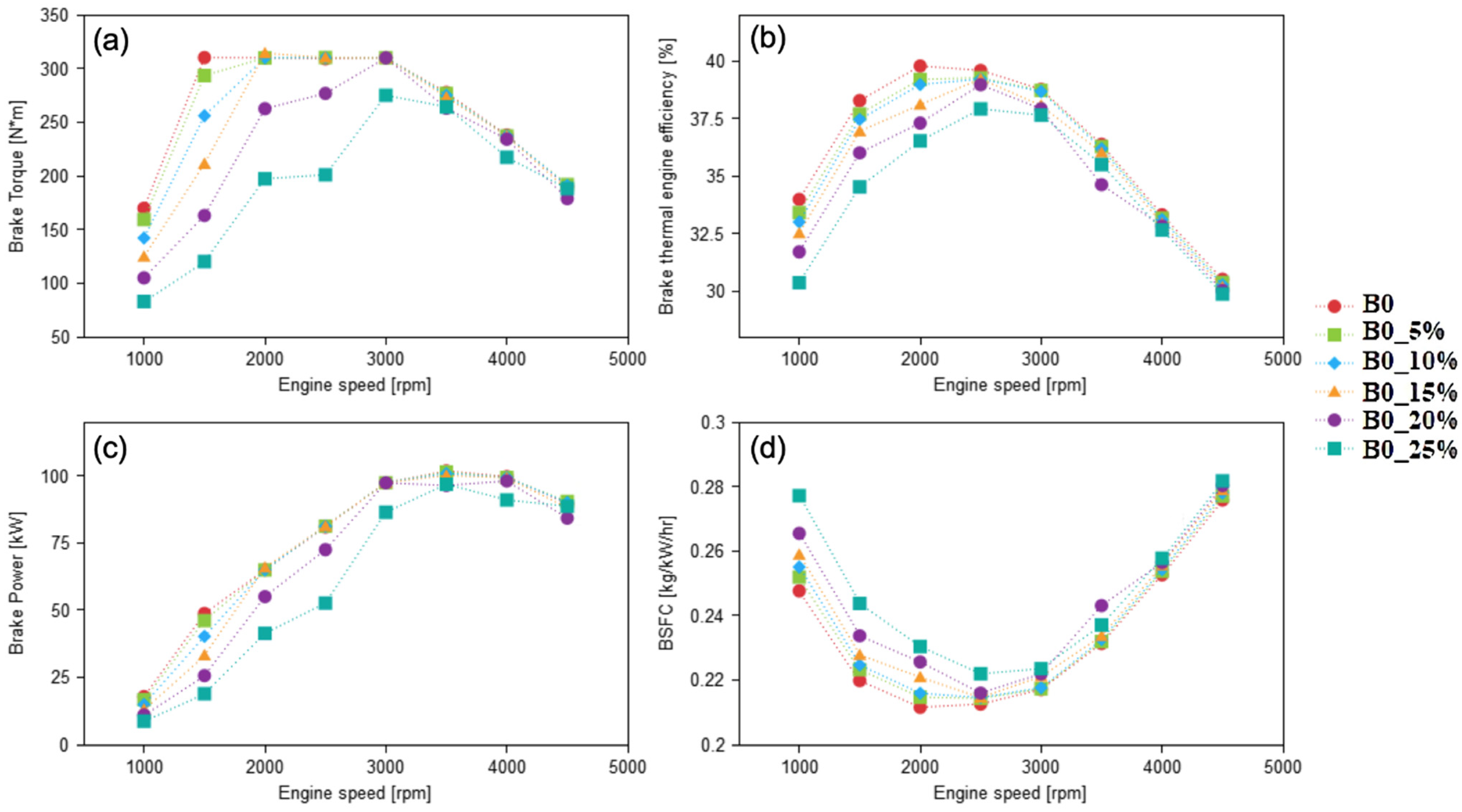
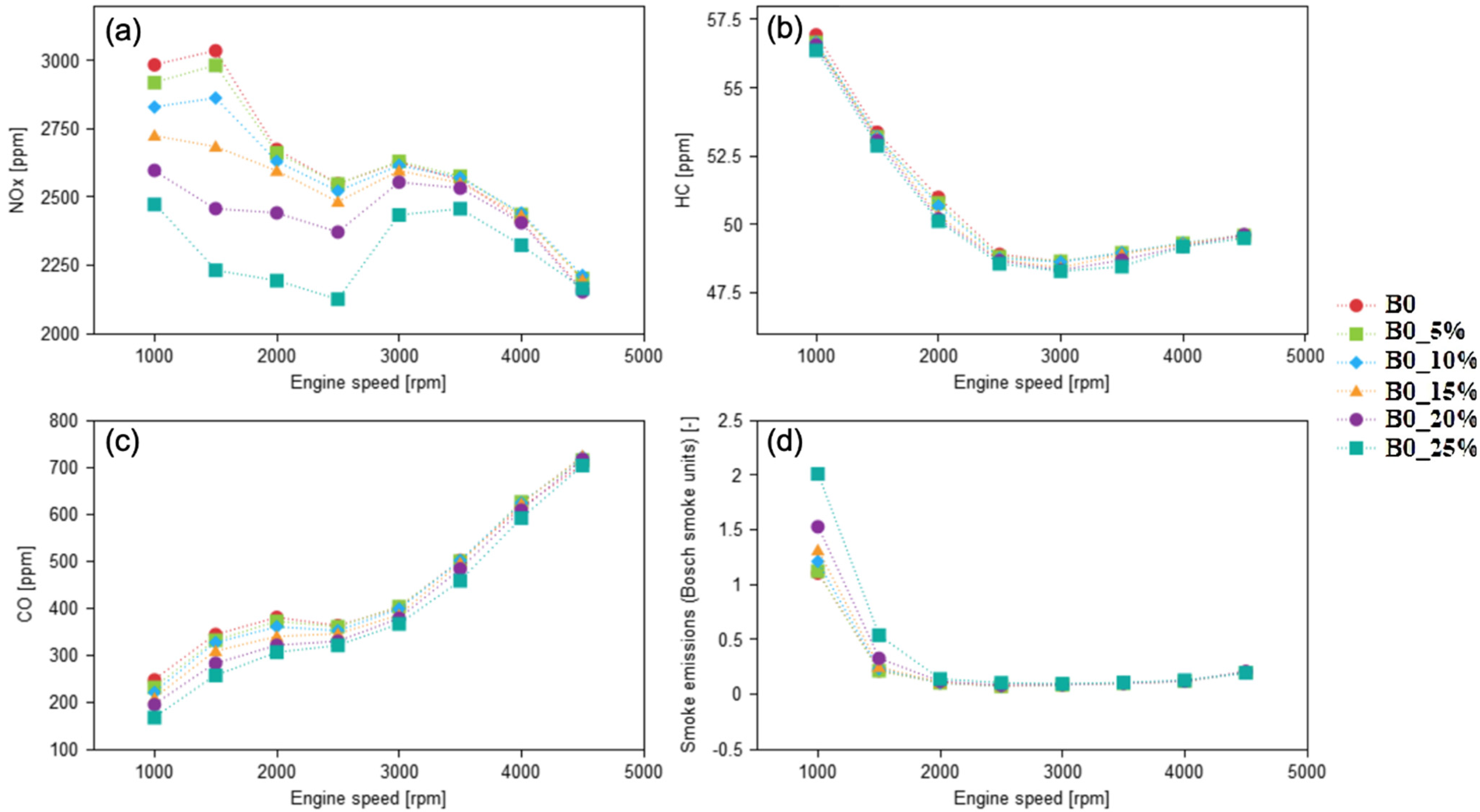
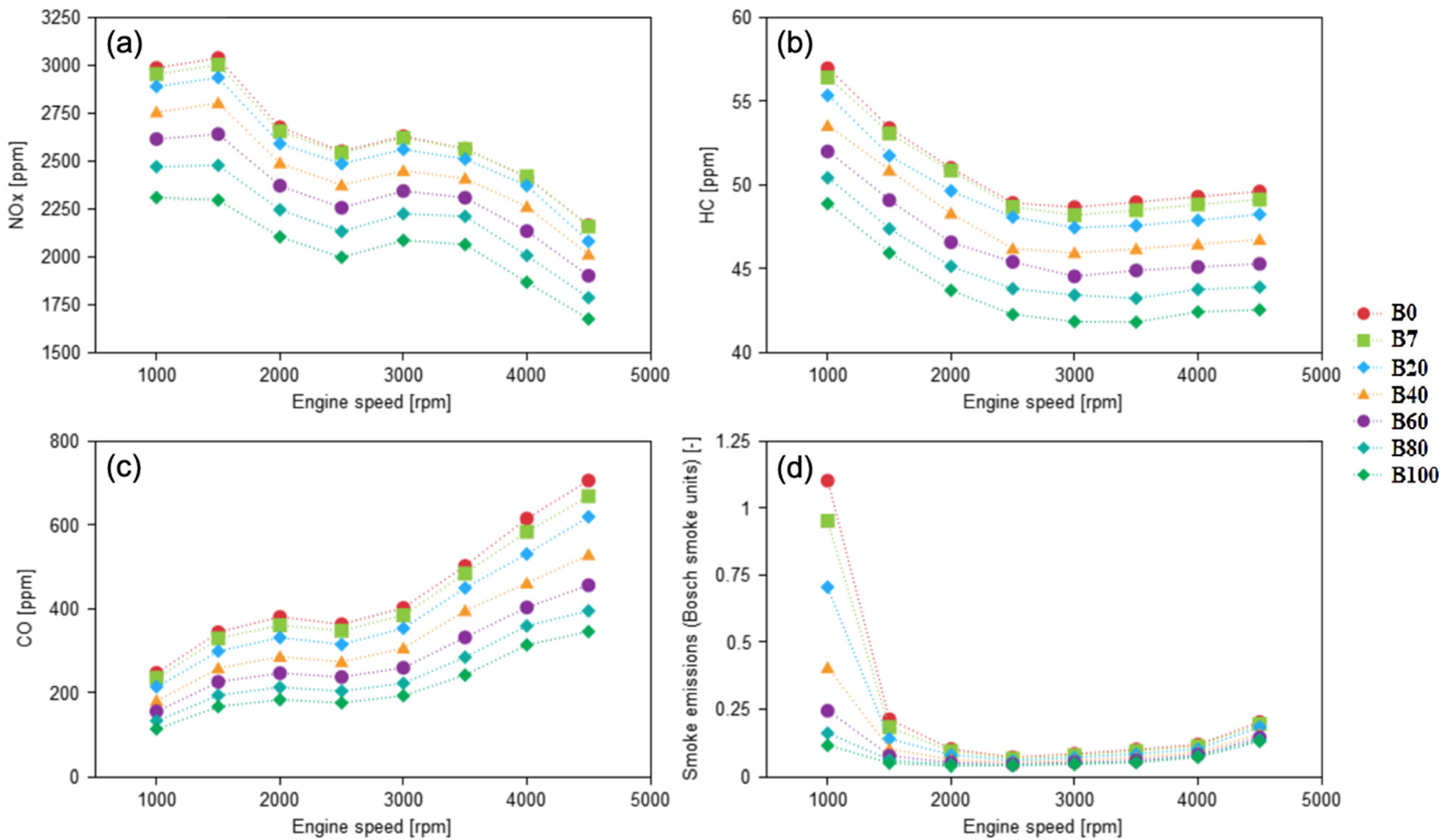
3.2. Effect of Varying Proportion Low-Carbon Fuels with No Miller Cycle

Table 5. The effect of changing the proportion of biodiesel on the performance and emissions at the rated speed compared to that of pure diesel (in %).

Fuel	Torque (%)	Power (%)	BTE (%)	BSFC (%)	NOx (%)	CO (%)	HC (%)	Soot (%)
B0	0	0	0	0	0	0	0	0
B7	−0.12	−0.12	0.11	0.69	−0.10	−3.09	−0.99	−6.70
B20	−0.50	−0.50	−0.12	2.41	−2.16	−10.00	−2.85	−17.31
B40	−1.09	−1.09	−0.68	5.41	−6.11	−20.89	−5.70	−30.29
B60	−5.52	−5.52	−4.43	12.19	−10.04	−33.62	−8.33	−40.79
B80	−1.66	−1.66	−3.47	13.81	−13.83	−43.10	−11.73	−46.75
B100	−5.01	−5.01	−5.40	19.07	−19.57	−51.66	−14.63	−49.27

shows the results at the rated engine speed (3500 rpm), with no Miller effect present. The results in Table 5 show a general decrease in torque, power, BTE, NO_x, CO, HC and soot, and an increase in BSFC as the proportion of biodiesel increases.

Figure 9 shows engine performance using different low-carbon fuels (diesel–biodiesel blends). The torque and power curves are relatively stable at mid-range engine speeds (2000–3000) rpm regardless of different fuel blends. However, the percentage of biodiesel starts to influence engine performance at either low or high engine speeds, since the torque and power losses increase with increasing biodiesel fraction. The maximum loss of 14.7% in power and torque is found at 1500 rpm for B100 compared to B0. Moreover, the difference between B0 and B20 is small, with a maximum decrease in power of 0.5% at 3500 rpm, but between B80 and B100 the difference in power increases to 3.3%.

The decrease of both power or torque is the most visible in B100 with the reductions of 11.0% and 14.5% at 1000 and 1500 rpm, respectively, and 13.1% and 9.5% at 4000 and 4500 rpm. This is mainly due to the lower energy content of biodiesel relative to mineral diesel, which means the less heat is released during the combustion of biodiesel. As a result, the engine produces less power.

There is a loss in BTE across almost all fuel blends and engine speeds, and this loss increases with increasing biodiesel percentage and increasing engine speeds. The BTE decreases by 0.5–1.0% for every 20% increase in biodiesel fraction, and reach average 2.5% for B100 across the whole range of engine speed.

The BSFC is also drastically affected by the fuel blends. Increasing the biodiesel fraction greatly increases BSFC, by 3% to 7% per 20% biodiesel increase. Unlike the power and torque curves, the increase in BSFC is generally stable across all engine speeds, which is attributed to the lower energy content (lower heating value) of biodiesel. There is an average 3% fuel consumption increase for each 20% increase in biodiesel, with a slight increase at the highest engine speeds. For B100, the BSFC is average 15.5% higher than that of pure diesel, with a peak of 19.6% at 3500 rpm.

The major advantage of biodiesel is the impact on emissions, as shown in Figure 10, there is decreases in all emission types as the proportion of biodiesel is increased. NO_x emissions are most significantly reduced in the lower engine speed range, whereas the reduced CO emissions occur to higher engine speeds. HC and soot emissions are evenly decreased across all engine speeds.

NO_x decreases as the proportion of biodiesel is increased, and the decrease is evenly distributed across all engine speeds. For example, B20 has on average 3% less NO_x emissions than B0, and B60 and B80 have nearly 5% decrease. The largest decrease is for B100, which emits an average of 22% less NO_x than B0. Table 5 shows this trend at the rated engine speeds. The lower NO_x emission from the low-carbon fuels is due to the lower heating value of the fuel.

CO emissions are more significantly influenced by biodiesel fraction than NO_x emissions. B20 shows reduced CO emissions by average 13% and by 10% at rated speed compared with B0. As the biodiesel fraction increases, CO emissions continue to drop, but the extent of reduction becomes smaller. For instance, the decrease from B80 to B100 is 8%, whilst that from B60 to B40 is 13%.

B100 experiences an average decrease in CO emissions of 51.9% across all engine speeds, and the decrease at rated speed of 51.7%.

HC emissions are more sensitive to varying biodiesel fraction than changing Miller cycle, and emissions decrease with increasing biodiesel fraction. HC emissions are reduced evenly across all engine speeds and experience a 3% decrease for each 20% increase in biodiesel fraction. The largest reduction occurs to B100, which has an average decrease in HC emissions of 14.1%, and a reduction at rated power of 14.6%.

Increasing biodiesel proportion has a noteworthy impact on soot emissions. By increasing the biodiesel proportion, soot emissions can be reduced significantly. The largest reduction is at lower engine speeds, with a peak value of 89.6% for B100 at 1000 rpm. The decrease in soot is not evenly distributed across all engine speeds. The decrease for B100 is 89.6% at 1000 rpm and 35.9% at 4500 rpm. The rate of reduction decreases as the proportion of biodiesel increases. Soot decreases by 20.8% between B0 and B20 and by 4.5% between B80 and B100. The average decrease over all engine speeds for B100 is 55.5% with 49.3% at rated speed.

The reason for the emissions of CO, HC and soot is mainly because the biodiesel contains oxygen atoms in it, which helps the combustion or oxidation process of the fuel, enabling more fuel to be burnt.

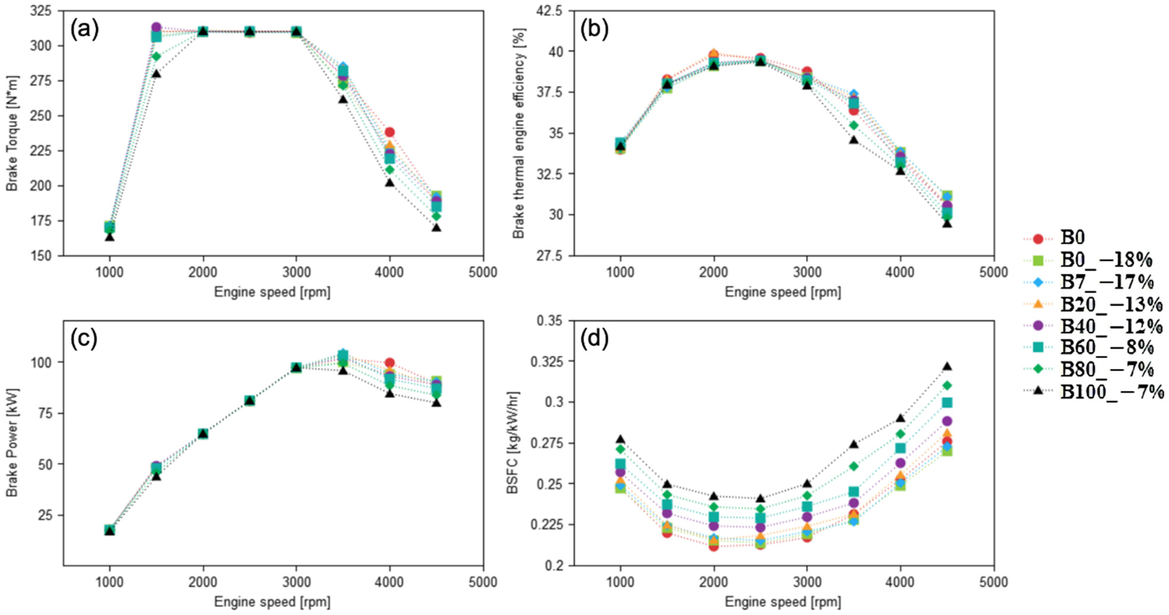
3.3. Combining Miller Cycle and Low-Carbon Fuels

From the trends of the engine performance found in Section 3.1 and Section 3.2 further investigation on the combined Miller cycle with biodiesel blends is carried out. A variety of different combinations is tested, i.e., combining a proper EIVC Miller cycle and one of the fuels selected, as shown in

Table 6. Optimal results found for each fuel tested, combined with the use of the Miller cycle (given in % difference to baseline engine at the rated speed).

Fuel	Miller Cycle (%)	Torque (%)	Power (%)	BTE (%)	BSFC (%)	NOx (%)	CO (%)	HC (%)	Soot (%)
B0	−18	−1.61	−1.61	1.49	−1.47	−8.99	−4.29	−1.10	21.27
B7	−17	2.69	2.69	2.81	−1.96	−7.48	−17.75	−2.03	9.59
B20	−13	2.08	2.08	2.27	0.03	−7.45	−21.24	−3.53	−6.01
B40	−12	0.22	0.22	1.70	2.95	−11.32	−31.56	−6.00	−20.14
B60	−8	1.50	1.50	1.19	5.96	−13.29	−38.54	−8.92	−33.02
B80	−7	−2.28	−2.28	−2.50	12.67	−16.45	−46.66	−11.87	−42.19
B100	−7	−5.81	−5.81	−4.94	18.49	−21.56	−54.31	−14.76	−46.91

. The results of the simulations are shown in Table 6 and Figure 11 and Figure 12.

Table 6 shows the optimal results for each fuel tested, combined with the Miller cycle used, at the rated engine speed (3500 rpm).

Table 6 illustrates that for the original (baseline) engine fuelled with pure diesel (B0), the optimal result is to use 18% EIVC Miller cycle. Under this condition, the brake thermal engine efficiency (BTE) could be improved by 1.49%, and the BSFC is reduced by 1.47%. Meanwhile, the emissions of NO_x, CO and HC are reduced by 8.99%, 4.29% and 1.10%, but soot is increased by 21.27%, with a minimum reduction of torque and power by 1.61%, respectively.

For the engine fuelled with B7, the optimal result is to use 17% EIVC Miller cycle. The torque, power and BTE could be improved by 2.69%, 2.69 and 2.81%, respectively. The BSFC is reduced by 1.96%, and the emissions of NO_x, CO and HC are reduced by 7.48%, 17.75% and 2.03%, but soot is increased by 9.59%, respectively.

For the engine fuelled with B20, the optimal result is using 13% EIVC Miller cycle. The torque, power and BTE could be improved by 2.08%, 2.08 and 2.27%, respectively, whilst the change in BSFC is negligible. The emissions of NO_x, CO, HC and soot are reduced by 7.45%, 21.24%, 3.53%, and 6.01%, respectively.

For the other combination cases, the optimal combinations are B40 with 12% of EIVC Miller cycle, B60 with 8% of EIVC Miller cycle, B80 with 7% of EIVC Miller cycle, and B100 with 7% of EIVC Miller cycle. In these cases, all of the emissions including NO_x, CO, HC and soot are reduced; although the BSFC increases by different extent in different case.

From Figure 11 and Figure 12, the trends of engine performance and emissions of the combined Miller cycle and different fuels can be identified:

(1)

At higher content of biodiesel where there is a power loss due to lower heating value of the fuel (as shown in Table 1), but use of the Miller cycle partially compensates for the loss of engine performance. For lower biodiesel content and for pure diesel the Miller cycle costs a small amount of engine performance, but at high biodiesel content the Miller cycle improves engine performance to a certain extent and reduces emissions. For example, without the Miller cycle, every fuel blend shows a decrease in power and torque. As shown in Table 6, for B7, B20, B40, and B60, using the Miller cycle improves both power and torque above the baseline. By using the Miller cycle, power and torque are also improved at lower engine speeds, which are more adversely affected by the use of low-carbon fuels. With B100 and no Miller cycle, there is a drop of 11.0% and 14.7% of power at 1000 rpm and 1500 rpm, respectively. When the Miller cycle is used at −7%, these losses are only reduced to 4.0% and 9.8%.

(2)

BTE is improved by an average of 3% compared with that of biodiesel without using Miller effect. For all fuel blends with biodiesel fraction up to B60, there is an overall increase in BTE compared to the baseline. There is still an improvement in B80 and B100 compared to biodiesel with no Miller effect, but the values are below the baseline engine.

(3)

When using Miller cycle, there are noticeable reduction in BSFC compared with biodiesel with no Miller cycle. The reduction varies from 1.1% for B100, to 6.2% for B60, and an average reduction across other fuel blends of 2–3%.

(4)

It is also found that, as biodiesel percentage increases, the Miller effect is further restricted due to the power loss. For example, by B100, the ideal Miller cycle percentage is found to be −7% (EIVC Miller Cycle), compared to −18% when B0 is used.

(5)

From Table 6 and Figure 11 and Figure 12, emissions are reduced with the combination of the Miller cycle and low-carbon fuels, compared to that in Table 5, Figure 9 and Figure 10. With optimal Miller cycle values, there is a minimum 2% reduction in NO_x emissions relative to biodiesel with no Miller effect, and more than 5% reduction with certain fuel blends such as B40.

Overall, the combination of Miller cycle and low-carbon fuel leads to an enormous improvement compared to the baseline. For B100 with no Miller effect, there is a 19.57% reduction in NO_x and 51.66% in CO relative to the baseline. With the optimal Miller cycle setup this is improved to 21.56% and 54.31%.

Similar results can be seen for the other low-carbon fuels, such as B20, where there are over 100% decreases in NO_x and CO emissions compared to B20 without the Miller Cycle at the rated speed. Even for the higher biodiesel fraction, where the effect is less noticeable, e.g., B80, there is a roughly 19% decrease in NO_x, and 8% decrease in CO emissions from the addition of the Miller cycle, respectively.

HC emissions are reduced with the addition of the Miller cycle, but to a less extent than NO_x or CO. There is an average decrease of 0.5–1.0% in HC emissions across all fuel blends when the Miller cycle is added.

All fuel blends with biodiesel fraction above 20% emit decreased soot emissions compared to the baseline. However, for B0 and B7, there is a negative effect by the addition of the Miller cycle. For example, with the optimal Miller cycle on B0, there is an average increase in soot emissions of 7.8%.

From Table 6, the overall optimal result has been identified; B60 with a −8% Miller effect. This gives an increase in power and torque of 1.5%, an increase in BTE of 1.2% at a cost of 6.0% of BSFC. Compared with emissions from the test engine burning standard diesel fuel without Miller cycle effect, the reduction is 13.3% for NO_x, 38.5% for CO, 8.9% for HC and 33.02% for soot emissions. This is an enormous reduction in all emissions while slightly improvement on the engine performance. Since the test engine used to develop the model is a Euro V diesel engine, the reduction in emissions means the optimal settings of biodiesel fraction and Miller cycle effect enable the engine to meet the Euro VI standards in terms of CO, HC and soot emissions, and the NO_x emission level will also be close to the Euro VI. Therefore, it is also rational to expect a significant reduction in emissions to Euro VI engines.

4. Conclusions

The effect of combined Miller cycle and low-carbon fuels on diesel engine performance and emissions is investigated using numerical models developed by Ricardo WAVE software. Simulations are carried out on Miller cycle up to ±25% (EIVC and LIVC) with seven diesel-biodiesel blends. The main conclusions are:

Miller cycle can reduce NO_x and CO emissions significantly (by 9.0% and 4.3%, respectively) and slightly improve BTE with the engine power loss no more than 1.6%. The BSFC and HC emissions are both reduced by 1.5%, whilst the soot emissions are significantly increased at rated engine speed.

Low-carbon fuels reduce all emissions with the cost of engine power loss, and reductions in emissions and power become more significant with increasing biodiesel fraction. The maximum engine power loss is 5.1%, whilst the NO_x, CO, HC and soot emissions are reduced by up to 19.57%, 51.66%, 14.63%, and 49.27%, respectively. Moreover, BTE and BSFC are negatively affected with a decrease of 5.4% and an increase of 19.1%, respectively.

Miller cycle can compensate for the performance loss caused by using low-carbon fuels whilst improving emissions. Therefore, the optimal crank timing (−8% EIVC) and biodiesel fraction (B60) are found for the combination of Miller cycle and low-carbon fuels to reduce all emissions and improve power, torque and BTE simultaneously compared to the baseline. This optimal configuration is recommended to implement on commercial diesel engines to obtain significant reduction in emissions at negligible costs in engine performance.

References

1. Hazel Clarke and David Ainslie; Office of National Statistics. ONS Road Transport Emissions. 2019. Available online: https://www.ons.gov.uk/economy/environmentalaccounts/articles/roadtransportandairemissions/2019-09-16 (accessed on 22 July 2020).
2. Wang, Y.; Zeng, S.; Huang, J.; He, Y.; Huang, X.; Lin, L.; Li, S. Experimental investigation of applying Miller cycle to reduce NOx emission from diesel engine. Proc. Inst. Mech. Eng. Part A J. Power Energy 2005, 219, 631–638. [Google Scholar] [CrossRef]
3. European Commission of Environment. Air Pollution from the Main Sources—Air Emissions from Road Vehicles. Available online: https://ec.europa.eu/environment/air/sources/road.htm (accessed on 21 December 2020).
4. Sydbom, A.; Blomberg, A.; Parnia, S.; Stenfors, N.; Sandström, T.; Dahlen, S.E. Health effects of diesel exhaust emissions. Eur. Respir. J. 2001, 17, 733–746. [Google Scholar] [CrossRef] [PubMed]
5. Jan Siczek, K. Tribological Processes in the Valve Train Systems with Lightweight Valves: New Research and Modelling; Butterworth-Heinemann: Oxford, UK, 2016; Available online: https://www.google.co.uk/books/edition/Tribological_Processes_in_the_Valve_Trai/Vz4oCwAAQBAJ?hl=en&gbpv=0 (accessed on 11 January 2022).
6. Naber, J.D.; Johnson, J.E. Internal combustion engine cycles and concepts. In Alternative Fuels and Advanced Vehicle Technologies for Improved Environmental Performance; Woodhead Publishing: Cambridge, UK, 2014; pp. 197–224. Available online: https://www.sciencedirect.com/science/article/pii/B978085709522050008X (accessed on 11 January 2022).
7. Wu, C.; Puzinauskas, P.V.; Tsai, J.S. Performance analysis and optimization of a supercharged Miller cycle Otto engine. Appl. Therm. Eng. 2003, 23, 511–521. [Google Scholar] [CrossRef]
8. Miller, R.H. Supercharging and internal coolimg cycle for high output. Trans. ASME 1947, 69, 453–457. [Google Scholar]
9. Balmer, R.T. Modern Engineering Thermodynamics-Textbook with Tables Booklet; Academic Press: Cambridge, MA, USA, 2011. [Google Scholar]
10. Xin, Q. Diesel Engine System Design; Elsevier: Amsterdam, The Netherlands, 2011. [Google Scholar]
11. Miller Cycle Application to the Scuderi Split Cycle Engine (by Downsizing the Compressor Cylinder). Available online: https://www.sae.org/publications/technical-papers/content/2012-01-0419/ (accessed on 11 January 2022).
12. Powell, N.; Little, M.; Reeve, J.; Baxter, J.; Robinson, S.; Herbert, A.; Mason, A.; Strange, P.; Charters, D.; Benjamin, S.F.; et al. Auxiliary power units for range extended electric vehicles. In Sustainable Vehicle Technologies: Driving the Green Agenda; Woodhead Publishing: Cambridge, UK, 2012; pp. 225–235. Available online: https://pureportal.coventry.ac.uk/en/publications/auxiliary-power-units-for-range-extended-electric-vehicles-2 (accessed on 11 January 2022).
13. Lin, J.-C.; Hou, S.-S. Performance analysis of an air-standard Miller cycle with considerations of heat loss as a percentage of fuel’s energy, friction and variable specific heats of working fluid. Int. J. Therm. Sci. 2008, 47, 182–191. [Google Scholar] [CrossRef]
14. Mikalsen, R.; Wang, Y.D.; Roskilly, A.P. A comparison of Miller and Otto cycle natural gas engines for small scale CHP applications. Appl. Energy 2009, 86, 922–927. [Google Scholar] [CrossRef] [Green Version]
15. Okubo, M.; Kuwahara, T. New Technologies for Emission Control in Marine Diesel Engines; Butterworth-Heinemann: Oxford, UK, 2019; Available online: https://www.google.co.uk/books/edition/New_Technologies_for_Emission_Control_in/OQ6sDwAAQBAJ?hl=en&gbpv=0 (accessed on 11 January 2022).
16. Watson, J.; Lotz, R.; Grabowska, D.; Moscetti, J.; House, T.; Scott, S.; Vemula, R. Development of a high-efficiency commercial-diesel turbocharger suited to post Euro VI emissions and fuel economy legislation. In Proceedings of the 11th International Conference on Turbochargers and Turbocharging, London, UK, 13–14 May 2014; pp. 13–14. [Google Scholar]
17. Praveena, V.; Martin, M.L.J. A review on various after treatment techniques to reduce NOx emissions in a CI engine. J. Energy Inst. 2018, 91, 704–720. [Google Scholar] [CrossRef]
18. Sindhu, R.; Rao, G.A.P.; Murthy, K.M. Effective reduction of NOx emissions from diesel engine using split injections. Alex. Eng. J. 2018, 57, 1379–1392. [Google Scholar] [CrossRef]
19. Güven, G.; Kayadelen, H.K.; Safa, A.; Sahin, B.; Parlak, A.; Ust, Y. Comparison of diesel engine and Miller cycled diesel engine by using two zone combustion model. INTNAM Symp. 2011, 17, 681–697. [Google Scholar]
20. Guven, G.; Sahin, B.; Parlak, A.; Ust, Y.; Ayhan, V.; Cesur, I.; Boru, B. Theoretical and experimental investigation of the Miller cycle diesel engine in terms of performance and emission parameters. Appl. Energy 2015, 138, 11–20. [Google Scholar]
21. Rinaldini, C.A.; Mattarelli, E.; Golovitchev, V.I. Potential of the Miller cycle on a HSDI diesel automotive engine. Appl. Energy 2013, 112, 102–119. [Google Scholar] [CrossRef]
22. Le, L.T.; van Ierland, E.C.; Zhu, X.; Wesseler, J.; Ngo, G. Comparing the social costs of biofuels and fossil fuels: A case study of Vietnam. Biomass Bioenergy 2013, 54, 227–238. [Google Scholar] [CrossRef]
23. United Kingdom Petroleum Industry Association. United Kingdom Petroleum Industry Association—Low-Carbon Fuels. Available online: https://www.ukpia.com/policy-focus/fuels/low-carbon-fuels/ (accessed on 18 December 2020).
24. An, H.; Yang, W.; Chou, S.; Chua, K.J. Combustion and emissions characteristics of diesel engine fueled by biodiesel at partial load conditions. Appl. Energy 2012, 99, 363–371. [Google Scholar] [CrossRef]
25. Karabektas, M. The effects of turbocharger on the performance and exhaust emissions of a diesel engine fuelled with biodiesel. Renew. Energy 2009, 34, 989–993. [Google Scholar] [CrossRef]
26. Wood, B.M.; Kirwan, K.; Maggs, S.; Meredith, J.; Coles, S.R. Study of combustion performance of biodiesel for potential application in motorsport. J. Clean. Prod. 2015, 93, 167–173. [Google Scholar] [CrossRef] [Green Version]
27. Zhang, J.; Jing, W.; Roberts, W.L.; Fang, T. Effects of ambient oxygen concentration on biodiesel and diesel spray combustion under simulated engine conditions. Energy 2013, 57, 722–732. [Google Scholar] [CrossRef]
28. Di, Y.; Cheung, C.; Huang, Z. Experimental investigation on regulated and unregulated emissions of a diesel engine fueled with ultra-low sulfur diesel fuel blended with biodiesel from waste cooking oil. Sci. Total Environ. 2009, 407, 835–846. [Google Scholar] [CrossRef]
29. Ban-Weiss, G.A.; Chen, J.; Buchholz, B.; Dibble, R. A numerical investigation into the anomalous slight NOx increase when burning biodiesel; A new (old) theory. Fuel Process. Technol. 2007, 88, 659–667. [Google Scholar] [CrossRef] [Green Version]
30. Mueller, C.J.; Boehman, A.L.; Martin, G.C. An Experimental Investigation of the Origin of Increased NOxEmissions When Fueling a Heavy-Duty Compression-Ignition Engine with Soy Biodiesel. SAE Int. J. Fuels Lubr. 2009, 2, 789–816. [Google Scholar] [CrossRef] [Green Version]
31. Kegl, B. Influence of biodiesel on engine combustion and emission characteristics. Appl. Energy 2011, 88, 1803–1812. [Google Scholar] [CrossRef]
32. Muralidharan, K.; Vasudevan, D. Performance, emission and combustion characteristics of a variable compression ratio engine using methyl esters of waste cooking oil and diesel blends. Appl. Energy 2011, 88, 3959–3968. [Google Scholar] [CrossRef]
33. Ricardo WAVE User Manual (Version 2020.3); Ricardo WAVE: West Sussex, UK, 2020.
34. Doric, J.; Klinar, I. Efficiency of a new internal combustion engine concept with variable piston motion. Therm. Sci. 2014, 18, 113–127. [Google Scholar] [CrossRef] [Green Version]
35. Ismail, H.M.; Ng, H.K.; Gan, S. Evaluation of non-premixed combustion and fuel spray models for in-cylinder diesel engine simulation. Appl. Energy 2012, 90, 271–279. [Google Scholar] [CrossRef]
36. Newhall, H.K. Kinetics of engine-generated nitrogen oxides and carbon monoxide. Symp. Combust. 1969, 12, 603–613. [Google Scholar] [CrossRef]
Figure 1. Miller cycle and standard cycle for diesel engine.
Energies 15 01783 g001
Figure 2. Schematic of the numerical model based on the test engine.
Energies 15 01783 g002
Figure 3. Model validation—comparison of (a) brake torque, (b) BTE, (c) brake power and (d) BSFC, between WAVE example model and baseline model.
Energies 15 01783 g003
Figure 4. Model validation—comparison of emissions (a) NOx, (b) HC, and (c) CO, and between WAVE example model and baseline model.
Energies 15 01783 g004
Figure 5. Comparison of (a) brake torque, (b) BTE, (c) brake power and (d) BSFC, for B0 LIVC operation.
Energies 15 01783 g005
Figure 6. Comparison of emissions (a) NOx, (b) HC, (c)CO, and (d) soot, for B0 LIVC operation.
Energies 15 01783 g006
Figure 7. Comparison of (a) brake torque, (b) BTE, (c) brake power and (d) BSFC, for B0 EIVC operation.
Energies 15 01783 g007
Figure 8. Comparison of emissions (a) NOx, (b) HC, (c) CO, and (d) soot, for B0 EIVC operation.
Energies 15 01783 g008
Figure 9. Comparison of (a) brake torque, (b) BTE, (c) brake power and (d) BSFC, with different diesel–biodiesel blends.
Energies 15 01783 g009
Figure 10. Comparison of emissions (a) NOx, (b) HC, (c) CO, and (d) soot, with different diesel–biodiesel blends.
Energies 15 01783 g010
Figure 11. Comparison of (a) brake torque, (b) BTE, (c) brake power and (d) BSFC, for different optimal setups.
Energies 15 01783 g011
Figure 12. Comparison of emissions (a) NOx, (b) HC, (c) CO, and (d) soot, for different optimal setups.
Energies 15 01783 g012